Discovering the Arrow of Time in Machine Learning

Abstract

Machine learning (ML) is increasingly useful as data grow in volume and accessibility. ML can perform tasks (e.g., categorisation, decision making, anomaly detection, etc.) through experience and without explicit instruction, even when the data are too vast, complex, highly variable, full of errors to be analysed in other ways. Thus, ML is great for natural language, images, or other complex and messy data available in large and growing volumes. Selecting ML models for tasks depends on many factors as they vary in supervision needed, tolerable error levels, and ability to account for order or temporal context, among many other things. Importantly, ML methods for tasks that use explicitly ordered or time-dependent data struggle with errors or data asymmetry. Most data are (implicitly) ordered or time-dependent, potentially allowing a hidden ‘arrow of time’ to affect ML performance on non-temporal tasks. This research explores the interaction of ML and implicit order using two ML models to automatically classify (a non-temporal task) tweets (temporal data) under conditions that balance volume and complexity of data. Results show that performance was affected, suggesting that researchers should carefully consider time when matching appropriate ML models to tasks, even when time is only implicitly included.

1. Introduction

Machine learning (ML) is a broad church. Supervised ML is very popular for exploring the relationship between clearly defined input and output variables. ML methods include: linear regression which handles continuous output by finding a line or plane that best fits the data, logistic regression which makes classification predictions for binary output, and support vector machines which classify by finding a hyperplane or boundary that maximises the margin between two or more classes. As an example, a supervised ML algorithm, or model, might be trained to classify incoming email based on the sender, subject line, or message content (input) that are accurately labelled as SPAM or NOT-SPAM (output). In contrast, unsupervised ML models attempt to draw inferences and find patterns from unlabelled data sets, such as finding neighbourhood clusters within demographic information. Common clustering methods include k-means clustering, which groups input into a pre-determined k number of groups, and hierarchical clustering, which arranges observations into tree-like graphs called dendrograms. For instance, an unsupervised ML model might be asked to classify research articles into disciplines according to their similarity. There are also semi-supervised approaches to machine learning, so the distinction is not always clear-cut.

ML models and tasks are diverse, but there are some general features that make some ML models useful for some tasks. For example, supervised ML can automatically classify items when the volume or complexity exceeds the capacity of manual classification or non-learning algorithmic exploration [1,2]. Similarly, unsupervised ML models are extremely useful for real-time data exploration and pattern detection in data that changes too quickly or too unpredictably for conventional exploration. ML (supervised and unsupervised) are often understood to perform better with more data. Nevertheless, there are trade-offs as unrepresentative data can lead to ‘over-fitting’ and poor generalisability, which is when a ML model performs very well on the training data but poorly on other data. ML is also typically understood to tolerate errors in the data, with some approaches showing acceptable performance despite error rates of up to 39 percent [1,2]. ML methods usually require substantial calculation, but this can be managed through careful selection of models and setups [3]. For these reasons, ML is understood to be a good tool for the large, complex, and messy data that are ballooning too rapidly for manual or conventional means of exploration, classification, or analysis.

This paper begins with some background on time, machine learning, and the intersection of the two. Following this is a clear description of the research question to be addressed and the methods and data used to address it. Next are the research results and a discussion of how the results relate to the research question. Finally, there is a brief discussion of what the results might mean for the wider ML research context and what potential next steps for this research topic.

1.1. The Arrow of “Time”

The “arrow of time” concept comes from 1927 theoretical physics lecture and describes the apparent one-way flow of time observed in irreversible processes at macroscopic levels. Although concluding that the arrow of time is a consequence of entropy, it was also described as a matter of perception, reasoning and statistical approaches [4]. Put another way, the one-way flow of time was understood to have a thermodynamic origin and psychological consequences. Thus, the arrow of time applies to irreversible processes that are both physical (e.g., an egg cannot be unscrambled) and economic or social (e.g., decisions cannot be undone and done differently instead), often known as path dependency or lock-in [5] as illustrated in Figure 1.

More recent work on the arrow of time maintains that people perceive and experience time as flowing in one direction, but highlights how the concept has continued to develop. Entropy is now linked to information and complexity [6] although the concepts and their applications are not interchangeable [7]. Currently, time’s arrow is thought to be a key driver of thermodynamic processes, biochemical processes like evolution via natural selection, and informational processes in both the natural world and cultural systems like language [6,8].

Setting aside the complicated concepts of information (especially as they related to entropy and thermodynamics), the arrow of time can be found in language; utterances (utterances are usually understood to be exclusively spoken, but this research counts tweets as utterances.) are spoken or written at a specific point in time. Further, language sequentially orders its components (symbols, semantic features, words, etc.) These temporal aspects of language are not always strict, allowing some meaning to be communicated ‘out of order’. Still, exactly what is communicated may not be “the same” as what would have been communicated if the utterances had been experienced at a different time or in another order. For example, classic literature is read and reread continuously with frequent new interpretations, all of which are probably unlike the contemporary interpretations from when the literature was originally available. Another example would be how readers may or may not struggle to understand the plot of a book series were they to read the sequel before the original. Likewise, some sentences can be understood more clearly than others when the words are jumbled; ‘eats mouse cheese’ is relatively clear while ‘eats man shark’ remains ambiguous.

The difference in interpretations or in interpretability described above derives from shared knowledge or common ground, which accumulates gradually as a consequence of experience [9]. Once learned, common ground allows communicators to recruit previously gained knowledge into helping interpret current utterances. Thus, books in a series can be read out of order if they deal with well-known topics, plots, tropes, events, or characters, even if they are not always interpreted in the same way. Likewise, individuals could use common ground to assume that the mouse is eating the cheese in the first jumbled sentence (rather than the cheese eating the mouse) but might not be able to make assumptions about the second without more context (as humans and sharks are both capable of eating each other).

However, common ground is also built between individuals through repeated interactions [9] and within a single interaction as participants take turns to speak and check their understanding [10]. Meaning is even built within a single utterance as linguistic input is incrementally processed word-by-word [10], which can create problems when an incremental understanding is violated by a ‘garden path’ sentence [11]. As a consequence, language use and comprehension are affected by prior exposure to language, most obviously in childhood language development where studies show neurological differences as a result of language exchanges and linguistic turn-taking [12].

1.2. Time in ML

ML includes supervised and unsupervised methods and can perform tasks such as prediction, classification, clustering, search and retrieval, or pattern discovery [13]. Some ML tasks, such as auto-complete word suggestions or weather warning systems, rely on using explicitly ordered or temporal data. Comparative studies have found that different ML models perform differently on time-series classification [14] and explicitly temporal tasks [15]; neural networks outperformed classic linear analysis techniques and multi-layer perceptron (followed by Gaussian processes) performing best across a range of categories and data features [16]. Clearly, ML can be very sensitive to time, with some ML models working with time better than others. Consequently, there are well-established data sets, benchmarks, and approaches for using ML models on tasks and with data that have an explicit order or temporal nature.

Many of the ML models that can deal with ordered or temporal data to address explicitly order- or time-sensitive tasks have problems or weaknesses that other ML methods can avoid. The problems of over-fitting and generalisability are more complicated because order/time is another dimension on which the data must be representative and which leaves the model relatively less tolerant of errors or missing values. Consequently, time-sensitive ML models typically have additional data requirements, including that the data must be organised into uniformly sized time intervals. Although not insurmountable, the stricter data requirements mean that time-sensitive ML is more difficult to apply or use. For tasks that do not require the specific use of time-sensitive methods, many researchers opt for ML models that assume the data to be time-independent and/or time-symmetrical.

Most of the data of interest for ML exploration and analysis are vast, complex, and messy because they are automatically generated by diverse digital technologies or practices. This means that the data of interest for ML usually have a temporal context. First, much of the data are time-stamped or otherwise ordered, although this is not always seen as important. Second, data are unevenly distributed over time as users, platforms, and records are added or shared, seriously complicating temporal representativeness. Additionally, features within these data are also unevenly distributed over time. To illustrate, 10–15% of medical diagnoses at any given point in time are estimated to be wrong [17], although which ones are erroneous is not known at the time. Some incorrect diagnoses are identified through later testing, condition progression, and medical innovations or discoveries, but the re-diagnosis is also subject to the 10–15% misdiagnosis rate. Further complicating the issue, a correct diagnosis according to the diagnostic criteria of the time could be a misdiagnosis according to later criteria. This becomes clear when we recognise that autism is not childhood schizophrenia [18] or that status lymphaticus is not a real condition [19]. Third, and perhaps most importantly, new data are not created independently of existing data. Instead, data are often generated as the result of learning from previously generated data. For example, users might change what content they share on a social media platform after observing what content is popular or well-received. When considered together, all of this suggests that the data that invite ML analysis are likely to be time-asymmetrical in ways to which many ML models are not well suited.

Researchers have begun to ask how time and ML models interact, both to correct for problems caused by temporal features, as well as to capitalise on these features. For example, sentiment analysis of Twitter data is well-established as a ML problem of interest, but accounting for temporal aspects of the data allowed researchers to analyse sentiment in ‘real-time’ tweets [20,21] while combining sentiment analysis of tweets with geo-tagging enabled researchers to build a spatial and temporal map of New York [22]. Further, using social interactions with temporal features allowed researchers to significantly improve stress detection in young people [23], potentially allowing problems to be detected early enough for effective intervention. Researchers have clearly noticed the ways that time is relevant to some ML models and some tasks and are beginning to investigate these interactions and even to put them to practical use. Thus, it is important to understand which models, tasks, or model–task pairs are sensitive to implicit temporal features and in what ways these temporal sensitivities affect the ML performance.

1.3. Research Question

This research addresses several related questions. First, will ML models performing automatic classification tasks be influenced, biased, or complicated by data with subtle or implicit representations of the flow of time? Put another way, how will ML models sort data differently when the assumption of time independence is violated? This could have consequences for how appropriate ML models are chosen according to the data available or the task to be performed.

A second problem would revolve around identifying, quantifying, or managing the ML model effects on typically non-temporal tasks when the data implicitly capture the one-directional flow of time. Researchers could always discard or reshape the data to meet the more stringent requirements of explicitly time-sensitive ML methods, weighting the data, presenting the data differently during training, or other possible modifications. While these may help balance the risks between over-fitting and implicit temporal distortion, it would leave the models relatively slow, fussy, and complicated which seems to lose many of the benefits of ML as it is currently understood. Alternatively, iterative learning could be introduced so that models learn from already-trained models, as well as from the data. By approximating the way that the people generating the data learn from past data, such iterative learning may account for the time-asymmetry of the data. Still, such potential changes may detract from the benefits of ML as it is currently understood or used.

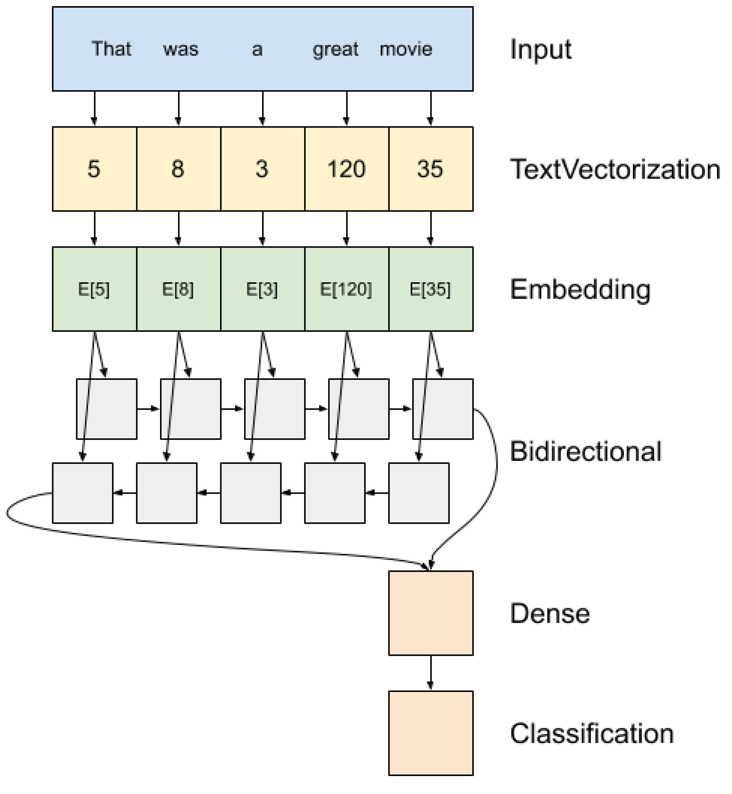
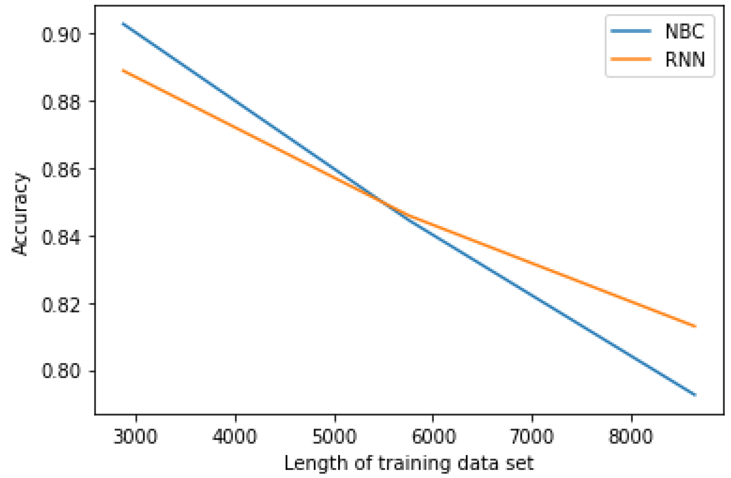
The research seeks to answer whether or not the ‘arrow of time’ can be observed in the performance of naive Bayes classification and recurrent neural networks ML models (both are commonly used) as they perform automatic classification tasks (very common) with Twitter data (a popular data source). Neither of these ML models are explicitly time-sensitive and so they do not have the sort of strict temporal representative measures of time-series prediction. Further, automatic classification tasks (e.g., sorting pictures into classes of ‘picture of a dog’ or ‘not a picture of a dog’) are not considered to be time-sensitive. The model will either accurately classify the pictures or not, regardless of when the picture was taken, when the classification happens, or how many pictures the ML model has been asked to classify. Finally, time is included in this data set, but not in a way that can be accessed directly. The model only has access to and learns from language and classifies purely based on the tweet text. This combination of model, task, and data are deliberately have no explicit access to or instruction to use time as a feature.

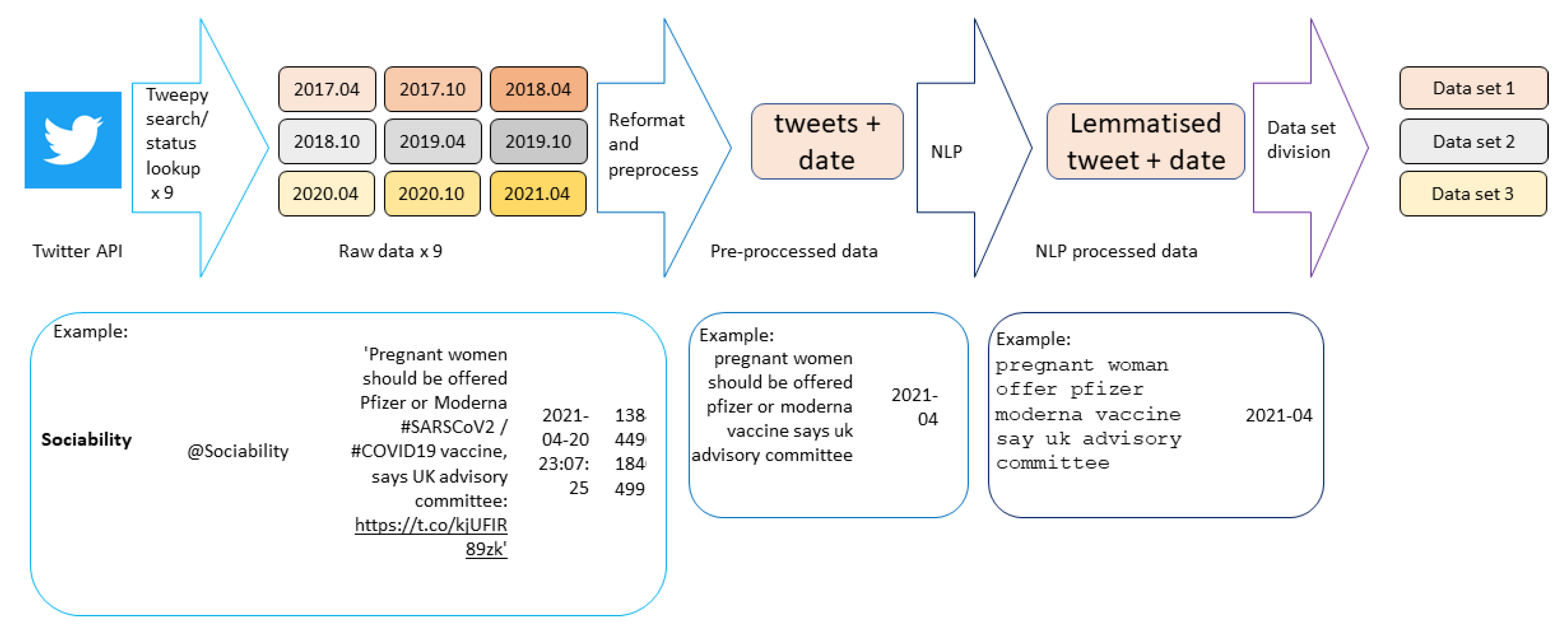
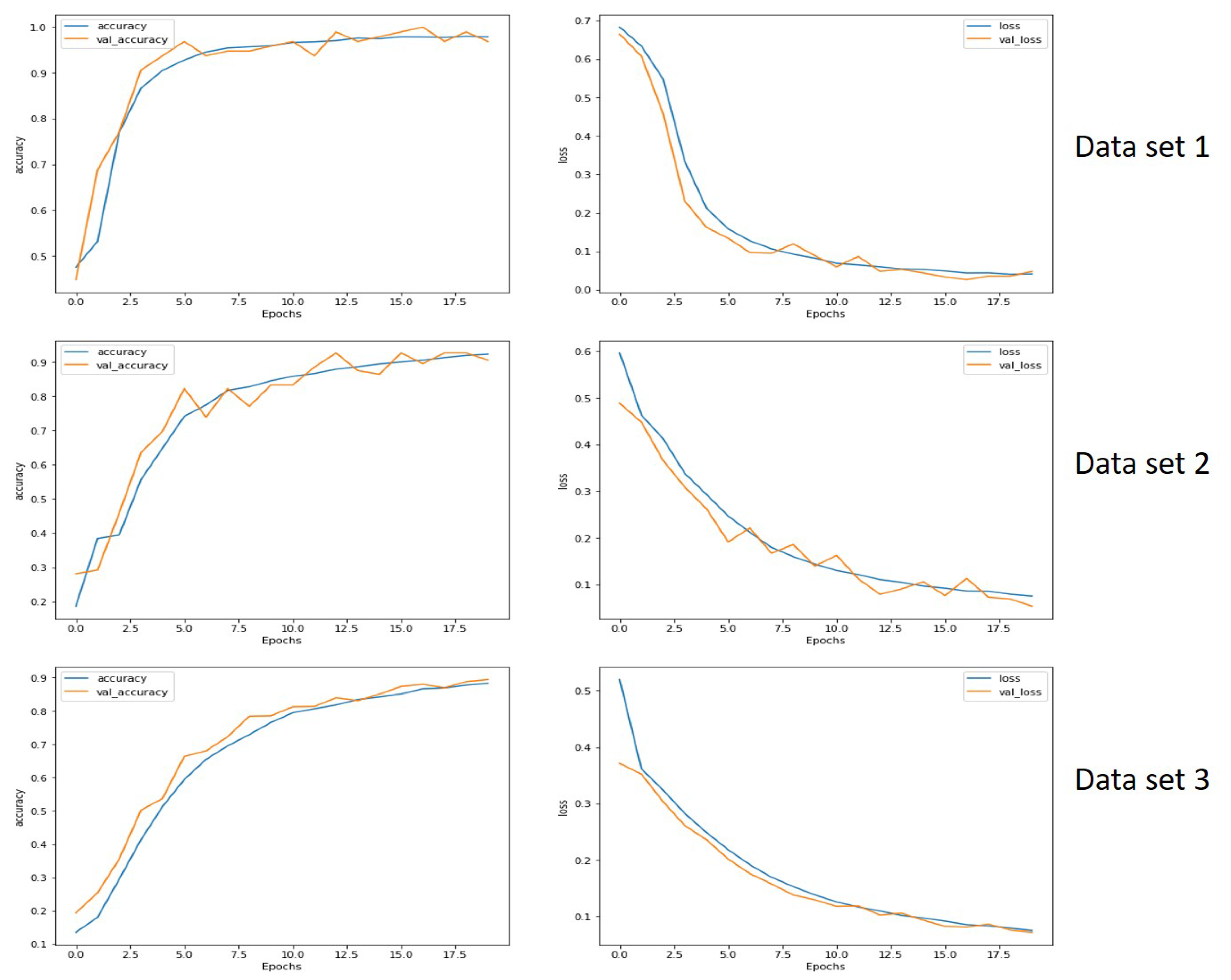
For extremely such common model–task–data combinations, more data are typically considered to be ‘better’ but that assumes that the data will not be complicated by an implicit arrow of time. The data in this case come from 9 searches, each of which covers a different time frame. The ML models are trained to classify by which search produced them, but are trained on 3 searches, 6 searches, and all 9 searches and which differ according to the time frame searched. If ‘more training data is always better’ then the performance should be equal or better when the models are trained on 6 or 9 searches in comparison to when they are trained on only 3. However, if the mode–task–data combination includes implicit temporal features that disrupt learning, then the performance should be worse on the models trained with more data than those trained with less. In essence, the research question can be rephrased as ‘is the performance of non-temporal ML models carrying out non-temporal tasks influenced by purely implicit temporal features of the data?’

2. Materials and Methods

This section describes the processes followed in this research, beginning with data collection and preparation, as depicted in Figure 2. This is followed by a description of the two supervised machine learning models chosen and how they are applied to the prepared data, as depicted in Figure 3 in order to perform the automatic classification. Finally, this section concludes with a description of how model performance was evaluated. The data, both raw and final, plus all the code used in the entire project are available through a GitHub repository [24].

As this research does not seek to improve any specific ML model, to close any given ML gap, or even to identify problems with any particular ML model, the researchers deliberately chose to use off-the-shelf code. Moreover, the steps taken, packages used, choices made (e.g., how to split the data into training and testing subsets), etc., are made to be as generic, basic, ‘entry-level’, or otherwise unimaginative. This helps keep the focus on the research.

2.1. Data

2.1.1. Collection

The data needed for this research must have two parts: the cleaned full text of tweets and the time frame of the search from which the tweet originally came. The ML models will use these data to learn to classify the tweets. However, the research question requires more than simply training and testing the models on such data. Instead, the ML models are trained and tested on subsets of the test data that encompass a small time frame, a medium time frame, and a large time frame. This allows the researchers to see if the models perform differently when the training sets vary by size and temporal complexity. In this way, the models can help illuminate whether more data is better (regardless of the temporal complexity of that data) or whether the greater language change and/or more numerous events captured within larger time frames distorts the way ML models can automatically classify tweets.

Data collection began by using the Tweepy [25] package and Twitter application programming interface (API) to collect tweets. The Tweepy search_full_archive and cursor methods take a start date, stop date, search keywords, maximum number, and an authentication environment parameters as input and returns truncated tweets with tweet ID, sender ID, tweet sent time and other details as output. For this research, we ran nine Tweepy searches with the keywords ‘vaccine’ and ‘UK’, maximum number of 1200, academic access as the authentication environment, and start and end dates that capture each six-month interval between April 2017 and April 2021 for a total of 10,800 tweets. For example, one search retrieved 1200 tweets published between 1 April and 20 April 2021 containing the keywords ‘vaccine’ and ‘UK’.

These 10,800 tweets were then passed through the Tweepy status_lookup method. This iterates over the IDs included in the initial Tweepy search results and replaces the truncated tweet text with the full tweet text, 100 at a time. This step is necessary as the text of the tweets is a key part of the envisioned data set.

It is important to note that this method requires a Twitter academic research developer account, which equips the user with the necessary API tokens to access Twitter materials and contents that are older than seven days. Applying for an academic developer account is free but requires explaining the purpose and planned use of the Twitter materials. Further, the search_full_archive developer environment within Tweepy must be set and labelled in the Twitter developer account portal.

2.1.2. Preparation

The Tweepy method described above produced nine ‘Twitter search result’ type objects which contain extraneous information and are not in the desired format or order. Thus, the output from each search is transformed into a table that retains only the ‘full_text’ and ‘created_at’ columns, with all other columns being dropped. The nine tables are then concatenated to create a single table with all of the data, after which the ‘Create_at’ values are re-coded to a simple year-month format. For example, a tweet originally dated ‘20 April 2021 23:07:35’ was re-coded to ‘April 2021’. The combined, reduced, and re-coded data are then saved and exported as a .csv.

Next, the Natural Language Processing (NLP) steps begin with the clean method from the ‘Preprocessor’ package [26] which removes URLs, hashtags, mentions, and reserved words (e.g., ‘RT’ for retweet or ‘FAV’ for favourite), emojis and smileys. Then, the sub method from the ‘Re’ package [27] removes punctuation and any words that appear in the English stop words list from the ‘NLTK.corpus’ package [28,29] (e.g., determiners, prepositions, pronouns, etc.) The tweets are then passed through the word_tokenize, pos_tag, get_wordnet_pos and lemmatize methods from the ‘WordNet’ functions, also from the ‘NLTK’ package [28,29]. This changes words to simple lemma versions according to how they were used in the original text so that ‘further’ and ‘farthest’ are both changed to ‘far’, ‘boxes’ is changed to ‘box’, and ‘recording’ is changed to ‘record’ if it was originally used as a verb but to ‘recording’ if it was originally used as a noun.

Then, the data set is copied and edited into three new data sets. Data set 1 contains only entries from the three most recent Tweepy searches (April 2020 to April 2021) and data set 2 contains only entries from the six most recent Tweepy searches (October 2018 to April 2021). Data set 3 contains all entries from all nine of the Tweepy searches (April 2017 to April 2021). These three data sets can be understood as three experimental conditions to see whether data set size and complexity influences automatic classification performance of one or both ML models.

2.1.3. Data Exploration

At this point, it is useful to briefly explore the post NLP data by search. Figure 4 presents word clouds that show the most frequent words from each, with the size of each word representing its frequency. Each of the searches is clearly unique and no two word clouds are the same although there are many words that appear in the word clouds for more than one search.

Comparing the word clouds shows differences linked to time in ways that are more or less obvious. For example, the influence of the global pandemic (still ongoing at time of writing) is clear from the size of words like ‘COVID’ or ‘COVID 19’ in the most recent searches and in how neither of these neologisms appears in older searches. It is clear that a global event can create or popularise new words and that the appearance and use of those words is related to the timing of the event and the subsequent discussions.

Similarly, ‘hpv’, ‘girl’, and ‘mmr’ feature strongly in the 2018.04 search and are present, but not as prominently, in other time periods. A bit of research showed that 2018 saw the HPV vaccine offered to preteen and teenage boys as well as girls and also featured unusually high rates of infection for measles, mumps, and rubella. Both of these events generated news articles, online discussions, and new behaviours, all of which are linked to the timing of policy changes and epidemiological spreading patterns. While the vaccine-related events in 2018 were not so memorable that the authors did not have to look for an explanation, they were nevertheless sufficient to have an temporally limited impact on Twitter discussions.

2.2. Modelling

Two ML models will be explored in this research: naive Bayes classifiers (NBC) and recurrent neural networks (RNN). Both are supervised ML models capable of automatically classifying many-to-one problems such as text-to-class. While both models take the same basic approach of learning from explicit training sets before being tested, exactly how they turn the three data sets that emerge from the data collection and preparation stage into model output is unique to each model as described below.

2.2.1. Naive Bayes Classification

An NBC ML model is a relatively simple, well-established method that is both efficient and effective [29]. Further, NBC models are frequently used as a baseline against which more complex models can be compared [30]. As a first step into an apparently unexplored area, we chose an NBC as the first ML model to test because it is appropriate for automatically classifying text data, has a straightforward and simple interpretation, and can serve as a standard for comparison. Specifically, automatically classifying strings of text into multiple categories requires a Gaussian NBC, which assumes that the data for each class are drawn from a Gaussian or normal distribution.

The NBC model process is straightforward; the lemmatised tweets are encoded as textblob objects via the TextBlob method from the ‘textblob’ [31] package. This converts them to lists of strings as input while keeping the date, or output, unchanged. The three data sets, now containing textblob objects and dates, are shuffled and divided into train and test sub-sets with an 80–20 split. Dividing a large data set into train and test subsets ensures that training and testing data are similar but contain no overlap.

NBC models learn to associate each word found in the training data input with the date output by creating and subsequently adjusting simple weighted associations. For example, if the first item of training data given to an NBC is [‘pregnant’ ‘woman’ ‘offer’ ‘moderna’ ‘vaccine’; ‘2021-04’], the model would record equally strong associations between all of the input words and the output date. If the next item of training data were [‘boy’ ‘girl’ ‘offer’ ‘hpv’ ‘vaccine’; ‘2018-04’], then the table would be updated to reflect the new words with strong associations, new and weaker associations for some existing words, and existing associations weakened where relevant. The outcome of learning from these two items of training data would look roughly like

Table 1. Initially uniform associations on the left and updated associations on the right.

Input	Output	Strength	Input	Output	Strength
‘pregnant’	‘2021-04’	1	‘pregnant’	‘2021-04’	1
‘woman’	‘2021-04’	1	‘woman’	‘2021-04’	1
‘offer’	‘2021-04’	1	‘offer’	‘2021-04’	0.5
‘moderna’	‘2021-04’	1	‘moderna’	‘2021-04’	1
‘vaccine’	‘2021-04’	1	‘vaccine’	‘2021-04’	0.5
			‘boy’	‘2018-04’	1
			‘girl’	‘2018-04’	1
			‘offer’	‘2018-04’	0.5
			‘hpv’	‘2018-04’	1
			‘vaccine’	‘2018-04’	0.5

. By the end of training, the words that are only paired to a single date would keep their strong associations while words paired to multiple dates (e.g., ‘vaccine’—an original search word) would have nearly uniform weak associations with all of the dates. Words that appear linked to some dates more than others would have medium strength associations that fall in between.

Importantly, this popular approach is often known as a or a ‘bag of words’ [32] because the order in which the words originally appeared has no consequence on how the model learns associations. In this way, an empty NBC model is trained on one of the three training data sets using the NaiveBayesClassifier method from the ‘textblob’ package, which uses the NBC function from NLTK [29] package. The trained NBC models are then tested on the corresponding test portions of the same data sets, so that the NBC trained on the train data from Data set 1 is tested on the test data from Data set 1, and so on. Testing is simply providing the trained model with a novel input, such as [‘woman’ ‘surgery’ ‘blood’ ‘clot’ ‘vaccine’] and asked to predict the correct date using the associations learned in training and maximum likelihood according the classic naive Bayes formula [29] as shown below. In this example, the model would (correctly) predict ‘2021-04’ on the combined strength of the associations between ‘woman’, ‘vaccine’ and ‘2021-04’ which win over the weaker association between ‘vaccine’ and ‘2018-04’.

$${\displaystyle P(date|Wor{d}_1\dots Wor{d}_n)=\frac{P(date)\ast P(Wor{d}_1|Date)\ast \dots P(Wor{d}_n|Date)}{P(Wor{d}_1)\ast \dots P(Wor{d}_n)}}$$

(1)

2.2.2. Recurrent Neural Networks

While NBC and other ‘bag of word’ models have many benefits, they do not always perform the best for all kinds of data [33]. Neural networks are more complex ML models that turn the input provided to a first layer into activation in subsequent layers according to the connections and weights, proceeding in this way with the activity of the final layer being interpreted as the predicted probability of output classes. The model then compares the predicted output to the real output in the training data and uses the difference to adjust the network connections and weights so as to reduce the error. Simple or feed-forward neural networks only accept a single input at a time so the information only flows in one direction but RNN models allow layers to feed their activation back to the previous layer so that input at any given step can contain input from the previous steps. For example, a feed-forward neural net might be fed a word one letter at a time with the aim of predicting the next letter; if fed ‘n’, ‘e’, ‘u’, ‘r’, and ‘a’, it would predict ‘n’ (statistically the most common letter to follow ‘a’). However, a RNN with the same task and inputs would predict ‘l’ because it would look at all of the letters in the input sequence rather than only the most recent.

RNN models use this looping structure to predict a single output, such as a date, from a complex sequence of inputs, such as text. The number and structure of the loops allows for variable memory, with long short-term memory RNN models (LSTM) solving the time-lag problem by considering inputs with long delays [34]. The ability to ‘remember’ and to solve problems with a time lag means that LSTM can be used to solve explicitly temporal tasks [35], although this research does not have such a task. Thus, the authors decided to use a LSTM RNN as the second ML model to test because it is appropriate for automatically classifying text data, has a more complex logic and function, and can provide a very different approach which can be compared to the NBC baseline. Specifically, we chose a bi-directional LSTM because it presents the entire training vector, both forwards and backwards, to two separate recurrent networks that share a single output layer—effectively considering the text as a whole when deciding on a single output.

As with the NBC, the RNN process begins by encoding the data sets into a format that the model can use. In this case, the lemmatised text is encoded as tensorflow-type data objects through tf.data.Dataset.from_tensor_slices function from the ‘Tensorflow’ package [36] and the ‘created_at’ dates are converted to a vector of binary features with one feature for each class in the data set get_dummies method from the ‘Pandas’ package [37]. For example, an item in Data set 1 (with three time periods) would convert the date ‘2021-04’ to [1 0 0] while an item in Data set 3 (with all nine time periods) might convert the date ‘2017.04’ to [0 0 0 0 0 0 0 0 1].

The encoded data sets are then divided into training and testing data subsets, again with a 80/20 split. Following this, the training data attached to the RNN model with the batch and prefetch functions, also ‘Tensorflow’ package [36], which help the model run smoothly and efficiently by controlling how often it should update its weights and whether to have a constant flow of input or move one item through at a time.

Once the training data are fully prepared, it passes through the 5-layer RNN model as depicted in Figure 5 multiple times, with each pass known as an ‘epoch’. The first layer uses experimental.preprocessing.TextVectorization and adapt methods from ‘Tensorflow’ to convert the input to a word index sequence that includes the frequency of each word within the specific data set. The second layer transforms the word index sequences to trainable vector sequences which, with sufficient training, turns different word sequences with similar meanings into similar vector sequences. The third layer is both important and complex as it contains the tf.keras.layers.Bidirectional wrapper, from the ‘Keras’ package [38], which propagates the vectors forward and backwards through the LSTM architecture.

The fourth and fifth layers all use functions from the ‘Keras’ package to predict the classification. The trained vector sequences are converted into a prediction vector via the tf.keras.layers.Dense and ReLu functions. The prediction vector has as many elements as there are classes (e.g., Data set 1 with 3 time periods has three elements) and the element with the highest score is interpreted as the prediction. The fifth and final layer uses the tf.keras.layers.Dense and softmax activation function to perform the final multi-class prediction by selection of the element from the prediction vector that has the highest value. All five layers are compiled using a categorical_crossentropy loss function and an adam optimiser function, also from the ‘Keras’ package.

Another important difference in how the two models learn relates to exposure. The NBC models get a single exposure to the train and test data sets, but only learns from the train data. In contrast, the RNN model gets multiple epochs or ‘passes’ through both the training and test data (again, only learning from the train data). The RNN adjusts its network weights with every epoch, making gradually smaller and smaller adjustments each time. Eventually, the learning plateaus and the model makes no further significant adjustments.

2.2.3. Testing

Testing the ML models is similar to the training with a key distinction; the model updates itself in light of the output value during training but not during testing. Instead, the predicted value during testing is compared to the real output value to determine how well the model performed.

There are many ways to measure performance, but the Python packages for both the NBC and RNN report ‘accuracy’ as simply the fraction of test data for which the predicted output is equal to the real output (Equation (2)).

$$Accuracy=\frac{|Y_{pred}=Y_{true}|}{|Y|}$$

(2)

As well as accuracy, the RNN also reports ‘loss’, which is the difference between the real output vector and the predicted output vector. To clarify, a real output vector might look like [1 0 0], while a predicted output vector might look like [0.8 0.2 0.0]. This predicted output vector can be interpreted to mean that the model is 80% certain that the tweet belongs to the first time period but finds a 20% chance that it could belong to the second time period. In this case, the ML model would have predicted the time period accurately, as the 80% certainty applies to the correct time period, but would have a loss score of 0.2 because of the differences between the predicted and correct output vectors.

3. Results

3.1. Overall Model Performance

Importantly, both the NBC and RNN models demonstrated good overall performance on categorising the tweets by time period. Accuracy, as described previously, is a simple measure of whether the ML model predicts the correct time period for each tweet in the test data for both models while loss is the difference between the correct output vector and the predicted output vector for the RNN. Accuracy for both models is shown graphically in Figure 6.

Table 2. Accuracy and loss results by data set and the length of all train and sets.

Data Set	Length		NBC	RNN
	Train Set	Test Set	Accuracy Score	Test Loss	Accuracy Score
1	2880	720	0.90	0.39	0.89
2	5760	1440	0.84	0.17	0.85
3	8640	2160	0.79	0.13	0.81

also reports the accuracy for both models, alongside the length of the train and test sets by data set and the loss for the RNN. The least accurate performance of any ML model in any experimental condition was just below 80%, suggesting that but selected ML models are capable of automatically classifying tweets into time period classes. It is important to reiterate that this task treats the time periods as simple categories into which the data must be classified. The time period categories in this case are equivalent to any other categories that might be used to train the ML models, such as sentiment, author, style, or anything else. This means that the ML classifiers used in these experiments have no explicit approach to time or order. Despite not having any explicit approach to time or order, there were some performance differences that suggest that both ML models are sensitive to the implicit ‘arrow of time’.

3.2. NBC Performance

The most accurate NBC model performance was over 90% and came from Data set 1. This was the data subset with only the three most recent time periods and thus the least data with which to train the ML model. Accuracy for the NBC model falls as more data are added, with Data set 2 showing 84% accuracy and Data set 3 falling just below 80% accuracy. Loss was not a metric generated by the NBC model used in this experiment, so accuracy is the only way to judge performance for this ML model.

3.3. RNN Performance

The RNN models show a similar pattern; accuracy drops as the volume of data and number of time periods in each data set increases. Data set 1, with only three time periods, was almost 90% accurate while Data set 2 was over 84% accurate and Data set 3 was just over 81% accurate. Figure 7 shows how the accuracy and loss functions changed across the twenty learning epochs. Accuracy and loss values from the train data (in blue) and test data (in orange) show how early phases make large jumps in performance by eventually levelling off with gradually less and less learning for each added epoch.

4. Discussion

An important result from both models is that accuracy was best for Data set 1 which contained fewer time periods and less data overall. This result is counter-intuitive in light of the commonly accepted idea that ML performance is improved by more data. Instead, this result supports the hypothesis that ML models which are not designed to account for or deal with temporal features or ordered data can still be influenced by an implicit representation of time. Interestingly, the fact that the NBC model showed this result suggests that even very simple non-temporal models can be disrupted by subtle or implicit temporal features.

At the same time, the drop in accuracy as data volume increased was not equal between the two models, indicating that not all ML models are equally disrupted by or equally adept at accounting for implicit representations of time. As the total accuracy drop was less pronounced for the RNN than for the NBC, RNN models may be less susceptible to subtle temporal effects or are better at capturing the complexity captured by data that spans greater time frames.

The learning functions for the RNN models show that the accuracy and loss for training and test data after each epoch are close, but not identical. Such non-identical similarity can be interpreted to mean that the models are well fitted to the data without suffering from over- or under-fitting. In contrast, if the performance was exceptional for the train data but poor for the test data, then the model would most likely be over-fit to the train data. These learning functions also reveal that handling more and more temporally complex data necessitates more iterations; learning for Data set 1 levelled off around the 10 epoch mark but the much larger Data set 3 required at least 20 epochs.

The results presented here could be explored further through other ML models, different or larger data sets (potentially with more specific geographical filtering), classification tasks that do not rely on predicting when a tweet was created, different ways to divide the data set into classes, and other training regimes. One particularly interesting training regime to explore would be ‘curriculum learning’ in which training data are fed into the model in a deliberate order (e.g., easy or straightforward training data first and then hard or more ambiguous training data later) [39]. In this way, additional interactions between ML and implicit representations of the ‘arrow of time’ may be discovered which might shed more light on the links between data complexity or temporal features and performance that can be achieved under different training regimes.

5. Conclusions

The main outcome of this research is that the results seems to contradict generally accepted ideas about ML; that more data is better and that classification tasks are not affected by time. Both models show that performance as measured by accuracy was not improved by making more data available. Instead, the results suggest that when the data contain implicit temporal features, having more data disrupts the capacity to classify. Effectively, implicit temporal data seem to be able to disrupt non-temporal ML models. Importantly, this research should be understood as a first step or ‘proof of concept’ rather than an exhaustive exploration of how ML and time interact. Classifying tweets into time periods is not a particularly important task, especially when Twitter data can easily be exported with a time stamp. Nevertheless, there are many important classification tasks that already routinely employ ML models, such as predicting diagnoses from medical images or identifying risk categories for individuals from their social media activity. These, and indeed most, classification tasks do not typically make use of time in the data or the analysis. Despite this, time is present in training data because it is created at a specific point in time (and within the technological and social context of that time). Likewise, the categories into which data is classified are also created, modified, or no longer used within clear temporal contexts. Thus, such classification tasks are inevitably influenced by time, even if the temporal representation is subtle or implicit. Importantly, the results of this research strongly suggest that the performance of ML classification tasks can be affected by subtle or implicit temporal features.

Currently, researchers weigh up many factors when selecting the appropriate ML model to use for a given research effort. These often include data volume, data complexity, generalisability, calculation costs, error tolerance, and many more factors because the characteristics of the data must be balanced against the aims of the research project. Time is only typically included in these factors to consider when the data or research question is explicitly temporal or ordered. Thus, the main conclusion of this research is that time should be added to the set of factors that researchers routinely consider when choosing which ML models to use. If they do not, an unacknowledged mismatch between the temporal features of the data and the ML model could have consequences on the total performance or training needs.

As it stands, the authors can only say that implicit time seems to matter for some classification tasks and that researchers should be aware of its potential effects on ML performance. Thus, the authors encourage researchers to consider the possible disruptions that may arise from a mismatch between non-temporal methods and implicitly temporal data when selecting a ML model. With further research, the authors would like to produce some more detailed guidance or heuristics to help in this selection process.

References

1. Brunk, C.A.; Pazzani, M.J. An investigation of noise-tolerant relational concept learning algorithms. In Machine Learning Proceedings 1991; Elsevier: Amsterdam, The Netherlands, 1991; pp. 389–393. [Google Scholar]
2. Kaiser, T.M.; Burger, P.B. Error tolerance of machine learning algorithms across contemporary biological targets. Molecules 2019, 24, 2115. [Google Scholar] [CrossRef] [PubMed] [Green Version]
3. Baştanlar, Y.; Özuysal, M. Introduction to machine learning. In miRNomics: MicroRNA Biology and Computational Analysis; Springer: Berlin/Heidelberg, Germany, 2014; pp. 105–128. [Google Scholar]
4. Eddington, A. The Nature of the Physical World: The Gifford Lectures 1927; Books on Demand: Norderstedt, Germany, 2019; Volume 23. [Google Scholar]
5. Page, S.E. Path dependence. Q. J. Political Sci. 2006, 1, 87–115. [Google Scholar] [CrossRef]
6. Mikhailovsky, G.E.; Levich, A.P. Entropy, information and complexity or which aims the arrow of time? Entropy 2015, 17, 4863–4890. [Google Scholar] [CrossRef] [Green Version]
7. Ben-Naim, A. Entropy, Shannon’s measure of information and Boltzmann’s H-theorem. Entropy 2017, 19, 48. [Google Scholar] [CrossRef] [Green Version]
8. Febres, G.; Jaffe, K. A fundamental scale of descriptions for analyzing information content of communication systems. Entropy 2015, 17, 1606–1633. [Google Scholar] [CrossRef] [Green Version]
9. CLARK, E. Common Ground; Wiley: Hoboken, NJ, USA, 2015; Volume 87. [Google Scholar]
10. Eshghi, A.; Howes, C.; Gregoromichelaki, E.; Hough, J.; Purver, M. Feedback in conversation as incremental semantic update. In Proceedings of the 11th International Conference on Computational Semantics, London, UK, 15–17 April 2015; pp. 261–271. [Google Scholar]
11. Ferreira, F.; Henderson, J.M. Recovery from misanalyses of garden-path sentences. J. Mem. Lang. 1991, 30, 725–745. [Google Scholar] [CrossRef]
12. Romeo, R.R.; Leonard, J.A.; Robinson, S.T.; West, M.R.; Mackey, A.P.; Rowe, M.L.; Gabrieli, J.D. Beyond the 30-million-word gap: Children’s conversational exposure is associated with language-related brain function. Psychol. Sci. 2018, 29, 700–710. [Google Scholar] [CrossRef] [PubMed]
13. Laxman, S.; Sastry, P.S. A survey of temporal data mining. Sadhana 2006, 31, 173–198. [Google Scholar] [CrossRef]
14. Bagnall, A.; Bostrom, A.; Large, J.; Lines, J. The great time series classification bake off: An experimental evaluation of recently proposed algorithms. Extended version. arXiv 2016, arXiv:1602.01711. [Google Scholar]
15. Wang, S.; Cao, J.; Yu, P. Deep learning for spatio-temporal data mining: A survey. IEEE Trans. Knowl. Data Eng. 2020. early access. [Google Scholar] [CrossRef]
16. Ahmed, N.K.; Atiya, A.F.; Gayar, N.E.; El-Shishiny, H. An empirical comparison of machine learning models for time series forecasting. Econom. Rev. 2010, 29, 594–621. [Google Scholar] [CrossRef]
17. Graber, M.L. The incidence of diagnostic error in medicine. BMJ Qual. Saf. 2013, 22, ii21–ii27. [Google Scholar] [CrossRef] [PubMed] [Green Version]
18. Kanner, L. Autistic disturbances of affective contact. Nerv. Child 1943, 2, 217–250. [Google Scholar]
19. Dodwell, H. “Status Lymphaticus,” the Growth of a Myth. Br. Med J. 1954, 1, 149. [Google Scholar] [CrossRef] [PubMed] [Green Version]
20. Goel, A.; Gautam, J.; Kumar, S. Real time sentiment analysis of tweets using Naive Bayes. In Proceedings of the 2016 2nd International Conference on Next Generation Computing Technologies (NGCT), Dehradun, India, 14–16 October 2016; pp. 257–261. [Google Scholar] [CrossRef]
21. Prakruthi, V.; Sindhu, D.; Anupama Kumar, D.S. Real Time Sentiment Analysis Of Twitter Posts. In Proceedings of the 2018 3rd International Conference on Computational Systems and Information Technology for Sustainable Solutions (CSITSS), Bengaluru, India, 20–22 December 2018; pp. 29–34. [Google Scholar] [CrossRef]
22. Bertrand, K.Z.; Bialik, M.; Virdee, K.; Gros, A.; Bar-Yam, Y. Sentiment in new york city: A high resolution spatial and temporal view. arXiv 2013, arXiv:1308.5010. [Google Scholar]
23. Zhao, L.; Jia, J.; Feng, L. Teenagers’ stress detection based on time-sensitive micro-blog comment/response actions. In Proceedings of the IFIP International Conference on Artificial Intelligence in Theory and Practice; Springer: Berlin/Heidelberg, Germany, 2015; pp. 26–36. [Google Scholar]
24. Zhao, A.; Kasmire, J. ICTeSSH-Arrow-of-Time, GitHub, 2021. Available online: https://assets.pubpub.org/cbyfgra4/51626784796909.pdf (accessed on 12 October 2021).
25. Roesslein, J. Tweepy: Twitter for Python! 2020. Available online: https://github.com/tweepy/tweepy (accessed on 1 May 2021).
26. Python Package Index-PyPI. Available online: https://docs.python.org/3/distutils/packageindex.html (accessed on 1 May 2021).
27. Van Rossum, G. The Python Library Reference, Release 3.8.2; Python Software Foundation: Wilmington, DE, USA, 2020. [Google Scholar]
28. Bird, S.; Klein, E.; Loper, E. Natural Language Processing with Python: Analyzing Text with the Natural Language Toolkit; O’Reilly Media, Inc.: Newton, MA, USA, 2009. [Google Scholar]
29. Zhang, H. The optimality of naive Bayes. In Proceedings of the 17th International Florida Artificial Intelligence Research Society Conference, Miami Beach, FL, USA, 12–14 May 2004. [Google Scholar]
30. Wang, S.I.; Manning, C.D. Baselines and bigrams: Simple, good sentiment and topic classification. In Proceedings of the 50th Annual Meeting of the Association for Computational Linguistics, Jeju Island, Korea, 8–14 July 2012; Volume 2, pp. 90–94. [Google Scholar]
31. Loria, S. Textblob Documentation. Python Package, Release 0.15. 2018. Available online: https://textblob.readthedocs.io/en/dev/ (accessed on 12 October 2021).
32. Lewis, D.D. Naive (Bayes) at forty: The independence assumption in information retrieval. In European Conference on Machine Learning; Springer: Berlin/Heidelberg, Germany, 1998; pp. 4–15. [Google Scholar]
33. Lee, S.H.; Levin, D.; Finley, P.D.; Heilig, C.M. Chief complaint classification with recurrent neural networks. J. Biomed. Inform. 2019, 93, 103158. [Google Scholar] [CrossRef] [PubMed] [Green Version]
34. Hochreiter, S.; Schmidhuber, J. LSTM can solve hard long time lag problems. In Proceedings of the Advances in Neural Information Processing Systems 9, NIPS, Denver, CO, USA, 2–5 December 1996; pp. 473–479. [Google Scholar]
35. Wang, F.; Xuan, Z.; Zhen, Z.; Li, K.; Wang, T.; Shi, M. A day-ahead PV power forecasting method based on LSTM-RNN model and time correlation modification under partial daily pattern prediction framework. Energy Convers. Manag. 2020, 212, 112766. [Google Scholar] [CrossRef]
36. Abadi, M.; Agarwal, A.; Barham, P.; Brevdo, E.; Chen, Z.; Citro, C.; Corrado, G.S.; Davis, A.; Dean, J.; Devin, M.; et al. TensorFlow: Large-Scale Machine Learning on Heterogeneous Systems. 2015. Available online: tensorflow.org (accessed on 12 October 2021).
37. The Pandas Development Team. Pandas-Dev/Pandas: Pandas. Zenodo, February 2020. Available online: https://pandas.pydata.org/about/citing.html (accessed on 12 October 2021).
38. Chollet, F. Keras, GitHub, 2015. Available online: https://www.scirp.org/(S(351jmbntvnsjt1aadkposzje))/reference/ReferencesPapers.aspx?ReferenceID=1887532 (accessed on 12 October 2021).
39. Bengio, Y.; Louradour, J.; Collobert, R.; Weston, J. Curriculum Learning. In Proceedings of the 26th Annual International Conference on Machine Learning, ICML’09, Montreal, QC, Canada, 14–18 June 2009; pp. 41–48. [Google Scholar] [CrossRef]
Figure 1. Path dependency illustrated in a simple graph; travel between points only moves in one direction (toward the future), after which previously accessible points (alternate futures) are longer available.
Information 12 00439 g001
Figure 2. The research process from collecting Twitter data through to analysis via the two different ML models, with examples of how an individual tweet appears at key stages.
Information 12 00439 g002
Figure 3. Both models follow similar steps using the 3 post-NLP data sets produced by the data collection and preparation steps. Each model encodes the data, splits it into training and testing subsets, and then applies the specific ML model processes to produce accuracy scores as output.
Information 12 00439 g003
Figure 4. Word clouds for each time period, labelled by the closing date of that time period.
Information 12 00439 g004
Figure 5. The RNN model has five layers, each of which serves a specific function.
Information 12 00439 g005
Figure 6. Accuracy scores for both models, plotted against the size of the training data set.
Information 12 00439 g006
Figure 7. Loss and accuracy functions from the RNN.
Information 12 00439 g007