Comparative Study of Dimensionality Reduction Techniques for Spectral–Temporal Data

Abstract

This paper studies the use of three different approaches to reduce the dimensionality of a type of spectral–temporal features, called motion picture expert group (MPEG)-7 audio signature descriptors (ASD). The studied approaches include principal component analysis (PCA), independent component analysis (ICA), and factor analysis (FA). These approaches are applied to ASD features obtained from audio items with or without distortion. These low-dimensional features are used as queries to a dataset containing low-dimensional features extracted from undistorted items. Doing so, we may investigate the distortion-resistant capability of each approach. The experimental results show that features obtained by the ICA or FA reduction approaches have higher identification accuracy than the PCA approach for moderately distorted items. Therefore, to extract features from distorted items, ICA or FA approaches should also be considered in addition to the PCA approach.

1. Introduction

It is very useful for many applications to reduce the dimensionality of data for higher processing speed, if the dimension-reduced data, also called features, can faithfully preserve important information from the original data. For example, in the feature-based object recognition problem [1], one important step, known as the feature extraction step, is to find a set of low-dimensional features to represent the underlying high-dimensional image. Doing so can significantly reduce the recognition time as well as storage space.

Another application of performing dimensionality reduction is to increase the processing speed. For example, a music identification system can significantly speed up the identification speed with the multi-resolution approach [2,3]. In this approach, a set of low-dimensional features is derived from the higher-dimensional features of a query audio clip. Based on the low-dimensional features, a small set of candidate objects are identified. Next, high-dimensional features are used to pick the best match among the chosen candidates. By comparing only a small set of candidates with high-dimensional features, the computational cost is dramatically reduced. However, to maintain high recognition accuracy, the low-dimensional features should have sufficient discriminant power. Thus, it is important to retain more useful information while performing dimensionality reduction.

In many applications, we use the short-time Fourier transform (or other time-frequency transformations) to observe the frequency characteristics of the signal along time [4] for a piece of signal, such as speech, music, or seismic wave. The computed coefficients, known as spectrogram, are a type of spectral–temporal features. Usually, this type of feature is arranged in a block (matrix) form, with one axis representing time and the other axis frequency. In this paper, the spectral–temporal features under consideration are the ISO’s (International Organization for Standardization) MPEG-7 (motion picture expert group) audio signature descriptors (ASD), which are shown to be effective for music identification (also to be covered in Section 2) [2,3,5].

The independent component analysis (ICA) [6,7] has been shown to effectively solve the cocktail-party problem, where several speech signals are mixed together. Recently, it is also used as a processing step in the recognition of EEG (Electroencephalography) waves [8,9]. Due to the underlying algorithm, components decomposed with ICA have the sign, scale, and permutation ambiguities. Therefore, we are unable to know which independent component has higher energy. With the scale ambiguity, it is not possible to choose the ICA-decomposed components based on component energy to perform dimensionality reduction. Therefore, we suggest an approach to walk around this difficulty and show the experimental results in this paper.

For many instances, we would like to investigate the factors affecting the observation. While this type of analysis can be carried out by the careful design of experiments, it can also be accomplished statistically by using factor analysis (FA). According to Reference [10], “… factor analysis is to describe the covariance relationships, if possible, among many variables in terms of a few underlying, but unobservable, random quantities called factors”. FA has many applications, such as anomaly detection [11,12]. Despite its popularity, only a few papers study the use of this method as a general dimensionality-reduction technique. In this paper, we will present our results of using FA as a reduction method and show the relative strength and weakness of this approach.

Although a complete survey of available dimension-reduction methods is available in the literature [13], unfortunately, the survey does not contain any quantitative comparison among the approaches. Previously, we have studied some dimensionality-reduction methods for MPEG-7 ASD, such as PCA (principal component analysis) [2,3]. In these papers, we use PCA, but not ICA or FA, to decompose the feature matrix, and then keep large components and discard smaller ones. Unfortunately, if an audio item is distorted, such as an air-recorded item, the distortion may also be present in large components. Therefore, the dimension-reduced features cannot faithfully preserve important information in the feature matrix. Previously, we have applied ICA for this problem and the results show that the ICA has better accuracy [14]. In this paper, we extend the work of Reference [14] to include FA in the comparison and to provide a detailed explanation for each of the compared approaches. To the best of the author’s knowledge, we have not read any paper conducting experiments with a similar comparison. In addition, although the experiments apply reduction techniques only to the MPEG-7 ASD, the presented approaches, nevertheless, are general approaches and can be easily applied to other types of features and application scenarios.

This paper is organized as follows: Section 2 covers the basics of the MPEG-7 features, which will be used in the experiments as the full-dimensional data. Section 3 describes how to perform dimensionality reduction with the PCA, ICA, and FA methods. Section 4 covers experiments and results. Finally, Section 5 is the conclusion.

2. Music Identification and MPEG-7 Audio Signature Descriptors

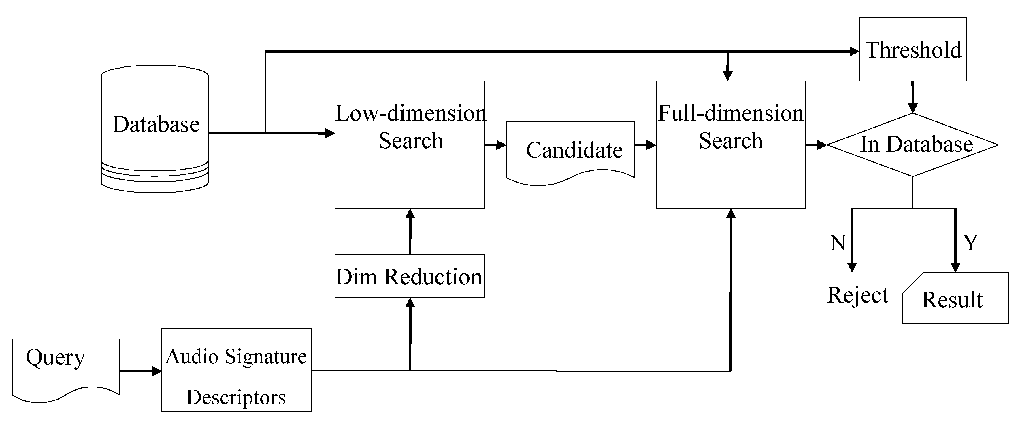
2.1. Music Identification

Music identification [2,3,15] is a technique to identify an audio clip from a large set of soundtracks based on the signal waveform. Therefore, even if the same person sings the same songs two times, these two audio works are considered as different. In terms of copyright protection, this distinction is actually an advantage, as there are many cover songs available in the market. Other applications of music identification also include query-by-exact example, broadcasting program monitoring, and so on [2].

Although the waveforms of different soundtracks are different, it is not possible to perform a comparison based on PCM (pulse code modulation) samples in the soundtracks because the computational cost is way too high [2]. Therefore, instead, we perform comparison based on some unique features extracted from the waveform. There are many proprietary schemes available to extract the features, as Shazam [16]. Other than the proprietary fingerprinting schemes, the ISO’s MPEG-7 audio standard also provides high-level tools to compute audio features suitable for music identification, known as audio signature tool. This tool computes ASD for each segment of the audio waveform. It is shown that the descriptors have satisfactory accuracy when used for music identification [2,3]. Unfortunately, as the dataset contains such a huge number of soundtracks, directly using the ASD would still require a lot of computation.

To cope with the high computational complexity, multi-resolution detection has been proposed [2], as shown in Figure 1. Firstly, low-resolution features are used to find a list of possible candidates. Second, the full-resolution features (fingerprints) are used only to compare the candidates in the list. By doing so, the computational cost can be greatly reduced.

2.2. Overview of MPEG-7 Audio Signature Descriptors

The MPEG-7 audio standard has many tools for audio feature extraction, audio identification, and audio recognition [5]. Some of the audio features are directly derived from the waveform of the audio signal. These low-level features can be used standalone or to construct high-level descriptors. The high-level descriptors may be used for more complicated tasks such as musical instrument recognition. In this paper, we use the ASD, one of the high-level descriptors, as the full-dimensional features to be reduced. To be complete, the computational steps of the ASD computation are given below.

• Perform time to frequency conversion. This step uses 4096-point FFT (fast Fourier Transformation) to obtain the spectral components of every segment of windowed audio samples. The chosen window is a Hamming window. The default window duration is 90 ms with 30 ms hopping step.
• Compute the flatness measure for each spectral band. A spectral band has a bandwidth of (1/4) octave, starting from 250 Hz and ending at 16 kHz. The flatness measure is the ratio of the geometric average to the arithmetic average of spectral components in a band.
• Computing the statistics of the flatness measure. Once the flatness measure is obtained, the final step is to compute the average and standard deviation (SD) of the measures over a period of time for each spectral band. The obtained average and SD values are called audio signature descriptors. In this paper, we only use the average values and discard the SD values in the experiments.

After the above computational steps, the obtained ASD can be represented in a matrix form, as depicted in (1), for a piece of 14-s audio. In the matrix, the horizontal direction represents frequency and the vertical direction represents time:

$$A=\left[\begin{array}{ccc}{a}_{1,1}& \cdots & a_{1,24}\\ ⋮& \ddots & ⋮\\ a_{29,1}& \cdots & a_{29,24}\end{array}\right]=\left[\begin{array}{ccc}\uparrow & & \uparrow \\ {\mathit{a}}_1& \cdots & {\mathit{a}}_{24}\\ \downarrow & & \downarrow \end{array}\right]$$

(1)

3. Dimensionality Reduction Approaches to Be Compared

3.1. Overview of 2-D PCA Computation

PCA has been widely used for reducing the dimensionality of features for many years [11]. In this paper, we have features arranged in a 2-D array form, not in a vector form. Therefore, we need to conduct the PCA reduction two times: first time in the vertical direction and the second time in the horizontal direction. For illustration purposes, we use the entire feature matrix to explain the computation steps. Suppose that the training dataset contains $A^{\left(1\right)},\cdots ,A^{\left(N\right)}$ feature matrices. To conduct PCA, we follow [17] and treat each column of $A^{\left(k\right)}$ as one measurement from a trail. By combining all $A^{\left(k\right)}$ together, we have the following matrix:

$$B=\left[\begin{array}{ccc}{A}^{\left(1\right)}& \cdots & A^{\left(N\right)}\end{array}\right]=\left[\begin{array}{ccc}\uparrow & & \uparrow \\ {\mathit{b}}_1& \cdots & {\mathit{b}}_{24N}\\ \downarrow & & \downarrow \end{array}\right].$$

(2)

In this representation, each column vector ${\mathit{b}}_k$ is one vector subject to be mapped to a lower-dimensional space. The PCA computational steps are as follows:

(a)

Remove means from the dataset. Let $\overline{\mathit{b}}$ be the vector of average for all ${\mathit{b}}_k$. We compute:

$${\mathit{x}}_k={\mathit{b}}_k-\overline{\mathit{b}}$$

(3)

to remove means. Note that it is not needed to make unity variances for elements in ${\mathit{x}}_k.$

(b)

Construct $X$ matrix as:

$$X=\left[\begin{array}{ccc}\uparrow & & \uparrow \\ {\mathit{x}}_1& \cdots & {\mathit{x}}_{24N}\\ \downarrow & & \downarrow \end{array}\right].$$

(4)

(c)

Decompose $X{X}^T$ matrix as:

$$X{X}^T=V\Lambda V^T,$$

(5)

where T denotes transpose, $\Lambda$ is a diagonal matrix containing eigenvalues of $X{X}^T$ arranged from large to small, and:

$$V=\left[\begin{array}{ccc}\uparrow & & \uparrow \\ {\mathit{v}}_1& \dots & {\mathit{v}}_p\\ \downarrow & & \downarrow \end{array}\right]$$

(6)

is an orthonormal matrix that contains the corresponding eigenvectors with $p = 29$

(d)

Use only $p = 3$ in (6) to perform reduction and denote the resultant matrix as $\tilde{V}$. Then, compute dimension-reduced matrix $R$, size of $24N \times 3$, from full-dimensional features $X$ by:

$$R=X^T\tilde{V},$$

(7)

(e)

After this step, the reduction in row direction of $A^{\left(k\right)}$ is complete. The next step is to perform a reduction in the horizontal direction. To do so, we treat $R^T$ as $X$ in (5) and repeat the computational steps one more time to complete the 2-D reduction.

In our previous paper, we have shown that a variation of 2-D PCA is slightly better. Thus, in the experiments, we use a slightly different method to compute the low-dimensional features [3].

3.2. ICA Reduction Technique

3.2.1. Introduction to ICA

The basic ICA algorithm consists of three main steps: centering, whiting, and maximizing non-Gaussianity [6,7]. Suppose that each ${\mathit{a}}_k$ in (1) is one vector subject to ICA, then the ICA is computed as follows.

(a)

Centering: Centering is to remove the average from the received samples. This step is equal to (3) in PCA.

(b)

Whitening: This step is used to remove the correlation between components through the covariance matrix. Its computational steps are similar to that of the PCA except a scaling. Specifically, we use:

$$\frac{1}{24N-1}X{X}^T=VD{V}^T$$

(8)

to compute the diagonal matrix $D$ containing eigenvalues. Then:

$${\mathit{z}}_k=V{D}^{-\frac{1}{2}}{V}^T{\mathit{x}}_k$$

(9)

is the resultant vector after the whiting step. It can be easily verified that if ${\mathit{z}}_k$ is an observation (outcome) of a random vector $\mathit{z}$, then $E\left\{\mathit{z}{\mathit{z}}^T\right\}=I$, where $E\{·\}$ is the expectation operation [6]. Note that (9) is used only to compute whitened measurements ${\mathit{z}}_k$. Further steps are necessary to obtain the transformation matrix to compute the final results.

(c)

Maximizing non-Gaussianity: Since we assume that the components of interests are not Gaussian distributed, it is natural to maximize non-Gaussian components. There are two widely used methods to measure the level of non-Gaussian, namely, kurtosis and negentropy. Please note that maximizing non-Gaussianity is not the only approach to perform ICA. Another widely used criterion is minimizing mutual information [7].

The kurtosis of a random variable $x$ is computed as:

$$Kurt\left(x\right)=E\left\{{\left(x-\mu \right)}^4\right\}-3·E{\left\{{\left(x-\mu \right)}^2\right\}}^2,$$

(10)

where $\mu$ is the mean value of $x$. According to (10), a Gaussian random variable has a kurtosis of zero. Therefore, the procedure of maximizing non-Gaussian is to maximize the absolute value of kurtosis. Specifically, let:

$$y={\mathit{w}}^T\mathit{z},$$

(11)

where the vector $\mathit{w}$ is a transformation vector. Note that we use the random vector $\mathit{z}$ in (11) because (10) involves the expectation operation. The objective function in this case is:

$$J_1\left(y\right)=\left|kurt\left(y\right)\right|.$$

(12)

The problem now becomes maximizing $J_1\left(y\right)$ with respect to a vector $\mathit{w}$ with $\Vert \mathit{w}\Vert =1$ for all observations of $\mathit{z}$, totally 24N vectors. If more than one component is needed, we can compute multiple $\mathit{w}$ vectors to form a transformation matrix $W$. This constraint optimization problem can be solved numerically, say, by fixed-point iteration.

The entropy of a random variable $x$ with a density function $f\left(x\right)$ is computed as:

$$H\left(x\right)=-{{\displaystyle \int }}_{-\infty }^{\infty }f\left(x\right)\log f\left(x\right)dx.$$

(13)

It can be shown that the Gaussian distribution has the highest entropy among all distributions. Based on (13), we define the differential entropy, or negentropy, as:

$$J_2\left(x\right)=H\left(x_G\right)-H\left(x\right)\ge 0,$$

(14)

where $x_G$ is a Gaussian random variable with the same variance as $x$. The goal of maximizing non-Gaussian can then be achieved by maximizing the negentropy. To use this concept, we let the objective function be $J_2\left(y\right)$, where $y$ is given in (11), and want to maximize $J_2\left(y\right)$ with respect to the vector $\mathit{w}$. In the practical implementation, (14) is difficult to compute. Therefore, we use an approximate equation, such as:

$$J_2\left(y\right)={\left[E\left\{G\left(y\right)\right\}-E\left\{G\left(v\right)\right\}\right]}^2,$$

(15)

where $v$ is zero-mean, uni-variance Gaussian random variable and $G$ is a function chosen from some candidate functions, such as:

$$G\left(y\right)=\frac{1}{\alpha }\log \cosh \left(\alpha y\right),$$

(16)

where α is a constant. The optimization problem in (15) can also be numerically solved by the fixed-point iteration algorithm.

3.2.2. Proposed ICA Reduction

As mentioned previously, the components obtained by the ICA has scaling ambiguity. Therefore, we are unable to directly use the ICA components with large energy as the dimension-reduced features. After second thoughts, we decide to reduce the dimensionality in the whitening step, detailed as follows:

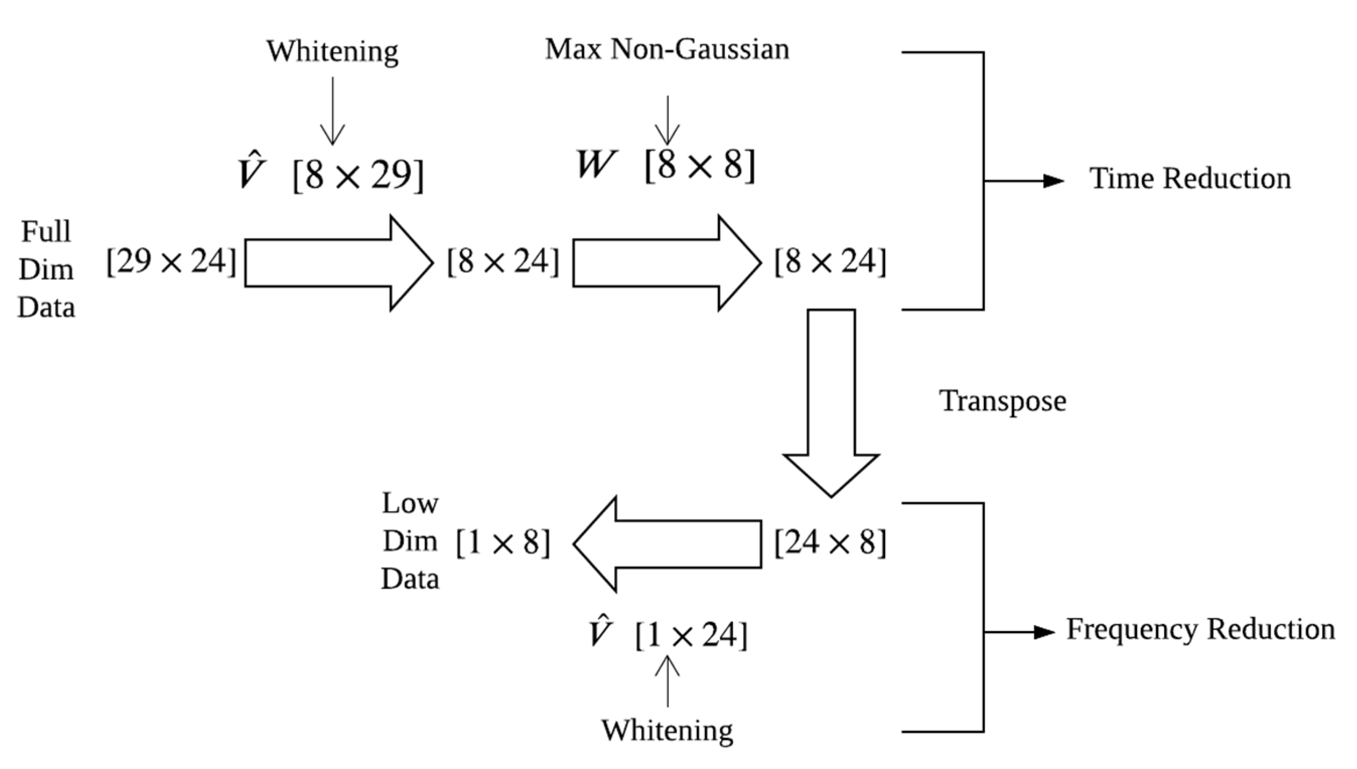
• Perform the centering and whitening steps. Simply following (8), we have:

  $$V=\left[\begin{array}{ccc}\uparrow & & \uparrow \\ {\mathit{v}}_1& \cdots & {\mathit{v}}_{29}\\ \downarrow & & \downarrow \end{array}\right].$$

  (17)
• Keep only eight components in $V$ to reduce the dimensionality. As before, the eigenvalues in (8) are arranged from large to small. Thus, we have a 29 × 8 matrix:

  $$\tilde{V}=\left[\begin{array}{ccc}\uparrow & & \uparrow \\ {\mathit{v}}_1& \cdots & {\mathit{v}}_8\\ \downarrow & & \downarrow \end{array}\right].$$

  (18)
• The next step is supposed to compute the whitening version of ${\mathit{x}}_k$. However, we are unable to use $\tilde{V}$ in the $V{D}^{-\frac{1}{2}}{V}^T$ term because $\tilde{V}$ is not a square matrix. To overcome this problem, we follow (24) in the proposed FA approach (to be discussed later), which in the present form is:

  $${\tilde{\mathit{z}}}_k={\left(\tilde{V}{\tilde{D}}^{\frac{1}{2}}\right)}^T{\mathit{x}}_k=\widehat{V}{\mathit{x}}_k,$$

  (19)

  where $\tilde{D}$ is a $8 \times 8$ diagonal matrix containing the eigenvalues associated with ${\mathit{v}}_j$ in (18), and ${\tilde{\mathit{z}}}_k$ has a size of $8 \times 1$. Recall that there are 24 ${\mathit{x}}_k$ vectors derived from one feature matrix $A$.
• Perform the maximizing non-Gaussianity step. In this step, eight $\mathit{w}$ vectors are obtained to form a transformation matrix $W$ (size of $8 \times 8$). Then, compute:

  $${\mathit{y}}_k=W{\tilde{\mathit{z}}}_k$$

  (20)
• Treat ${\mathit{y}}_k$ as ${\mathit{x}}_k$ and repeating the whitening procedure again. However, this time we keep only one vector in (18) to compute the final low-dimensional features.

The sizes of matrices involved in the proposed ICA approach are given in Figure 2. The $\widehat{V}$ matrix is computed from (19) and the $W$ matrix is from non-Gaussian step. Recall that the computation of $\widehat{V}$ is closely related to the PCA approach. Therefore, the ICA reduction is an extension of the PCA approach, with the maximum non-Gaussian step in between two PCA computations.

3.3. Overview of 2-D FA Computation

3.3.1. Introduction to Factor Analysis

Factor analysis includes exploratory factor analysis and confirmatory factor analysis [18,19]. In this paper, we only consider exploratory factor analysis [20]. In addition, there are many different types of factoring, such as principal component analysis and canonical factor analysis [12]. We use the principal component analysis method in this paper. This type of factor analysis is also called principal component factor analysis [12].

Suppose that there are m observable random variables, $x_1$ to $x_m$, with respective mean values of ${\overline{x}}_1$ to ${\overline{x}}_m$ under investigation. Furthermore, suppose that there are unknown constants ${\ell }_{i,j}$ with unobservable random variables $e_j$ with i from 1 to m and j from 1 to n, where n is less than m. We then can have the following expression:

$$\left[\begin{array}{c}{x}_1-{\overline{x}}_1\\ ⋮\\ x_m-{\overline{x}}_m\end{array}\right]=\left[\begin{array}{ccc}{\ell }_{1,1}& \cdots & {\ell }_{1,n}\\ ⋮& \ddots & ⋮\\ {\ell }_{m,1}& \cdots & {\ell }_{m,n}\end{array}\right]\left[\begin{array}{c}{e}_1\\ ⋮\\ e_m\end{array}\right]+\left[\begin{array}{c}{\zeta }_1\\ ⋮\\ {\zeta }_n\end{array}\right],$$

(21)

where ${\zeta }_j$ is random noise. Sometimes, we write (21) in short form as:

$$\mathit{x}-\overline{\mathit{x}}=L\mathit{e}+\mathit{\zeta }.$$

(22)

It is a common practice to assume that $\mathit{e}$ and $\mathit{\zeta }$ are independent, ${\overline{e}}_j=0$, and the covariance matrix of $\mathit{e}$ is the identity matrix. In addition, all random variables in $\mathit{\zeta }$ are independent with finite variances. To find any solution to (22), we add additional constraints to obtain [13]:

$$\mathrm{Cov}\left(\mathit{x}\right)=L{L}^T+\mathrm{H},$$

(23)

where Cov(•) denotes the covariance matrix and $\mathrm{H}$ is the covariance matrix of $\mathit{\zeta }$. As $\mathit{\zeta }$ contains independent random variables, $\mathrm{H}$ is a diagonal matrix. The computed $\mathit{e}$ is called the factors and L is called the loading matrix.

3.3.2. Proposed FA Reduction

To use FA, we need to find the loading matrix $L$. By using the principal component factor analysis [8], the steps to compute the proposed FA reduction approach are given below.

(a)

Follow the ICA computation in (17) to obtain $V$ matrix, and then choose $p$ components to construct $V_p$ matrix.

(b)

Construct the loading matrix $\widehat{L}$ by:

$$\widehat{L}=\left[\begin{array}{ccc}\uparrow & & \uparrow \\ \sqrt{{\lambda }_1}{\mathit{v}}_1& \cdots & \sqrt{{\lambda }_p}{\mathit{v}}_p\\ \downarrow & & \downarrow \end{array}\right].$$

(24)

In the simulation, we use $p=3$.

(c)

Compute the factor scores for one vector ${\mathit{x}}_k$ by:

$${\mathit{f}}_k={\left({\widehat{L}}^T\widehat{L}\right)}^{-1}{L}^T{\mathit{x}}_k.$$

(25)

Then, the obtained ${\mathit{f}}_k$ is a dimension-reduced vector in one direction (i.e., time information is lost).

(d)

To further reduce the dimensionality of the features in another direction, we perform the same steps a second time by treating ${\mathit{f}}_k$ as ${\mathit{x}}_k$.

When completing the procedure, we have an $3 \times 3$ matrix as the factor scores for one feature matrix $A$. In the simulation, we discard the element of $\left(3,3\right)$ and use the rest of 8 elements.

4. Experiments and Results

4.1. Experimental Settings

The experiments were carried out by computer simulations. To do so, we collected 750 soundtracks with various genres from different CD titles. The genres of the soundtracks included classical music, piano solo, soft music, pop music, and so on. The duration of each excerpted soundtrack was 30 s. These soundtracks served as the reference (database) items. Next, testing (or query) items with a duration of 15 s were excerpted from the reference items with random starting points. We used random starting points to simulate the actual recording situation. These items were referred to as the original testing items. The original testing items were subject to some widely encountered distortion attacks, such as audio compression and recording, to be described below.

To evaluate the detection accuracy after audio compression, we encoded the original test items with MP-3 (MPEG-1 layer 3) [21] in 192 kbps (kilo bit per second) and 96 kbps bitrates, respectively. As the original test items were stereo audio, they were encoded in the joint stereo mode. Then, the compressed items were decoded to PCM items. These items were downmixed from stereo to mono before testing.

To further investigate the identification accuracy under the actual recording environment, we also collected recorded items. Specifically, we played the original test items with a notebook and recorded the audio signal through two different paths, as shown in Figure 3. In the first path, the audio output port of the notebook is directly connected to the audio input port of a desktop computer. Thus, the signal-recording path contains a digital-to-analog converter, an analog-to-digital converter, and associated anti-aliasing and reconstruction filters. The obtained testing items are called wire-recorded items in the following. In the second path, the audio item is played back through a loudspeaker, and the acoustical signal is recorded by a microphone. The test items recorded with the microphone are referred to as the air-recorded items. Another set of testing items are obtained by adding −20 dB and −10 dB AWGN (additive white Gaussian noise) to the original testing items. The noise energy is relative to the signal energy.

The reason that we used both wire and acoustic recordings is to study the impact of the distortion sources. For wire-recorded signals, the distortion is mainly due to the signal processing blocks inside the personal computer, such as the anti-aliasing filter and the analog-to-digital converter. Thus, the amount of distortion may be reasonably small. For the air-recorded items, the distortion sources include the loudspeaker distortion, the room impulse response, the ambient (environmental) noise, and possibly the microphone response. When compared with the wire-recording items, it is reasonable to guess that air-recorded items have much higher distortion.

Before conducting the identification task, the reference items and all sets of testing items were converted to MPEG-7 ASD. To have the highest possible accuracy, the high-frequency bands (higher than 4 kHz) were removed before reduction [2,3]. These descriptors are referred to as full-dimensional (FD) features. Next, low-dimensional features were obtained from the FD features by using the PCA, ICA, and FA approaches mentioned in Section 3. Finally, the low-dimensional features were presented as queries to the database as the testing items. Recall that the database contains only undistorted reference items.

The identification of a query item is carried out based on similarity, which is the Euclidean distance between a reference item and the query item. From Figure 1 we know that whether a query item is inside or outside the database is determined by using FD features, therefore, all LD query items are assumed to be excerpted from the reference items. The performance measure of the reduction approaches is based on accuracy. A candidate list is constructed based on the first i-th shortest distances. For example, the 15-th list contains 15 song titles. If the test item is actually in the list, the item is called correctly identified. By doing so, we can compute the accuracy. Recall that the low-dimensional features are used only to find candidates in the multi-resolution approach, and full-dimensional features will be used to identify the test item among the candidates. Thus, practically it is more important to consider the accuracy in the, say, 15-th match than in the 1-st match. Furthermore, in the present application, it is not so much useful to compute the average ranking for a method.

4.2. Comparison between Kurtosis and Negentropy Criteria

Because there are two widely used criteria to maximizing non-Gaussianity in computing ICA, we would like to know if these two have comparable performance. We know that a query item is more difficult to identify if it has some distortion. To this end, we compute the low-dimensional query items using these methods for test items that undergone MP-3 compression. The accuracy between the kurtosis and the negentropy approaches is given in

Table 1. Identification accuracy between kurtosis and negentropy in ICA.

Distortion	i-th Match	Kurtosis	Negentropy
192 k MP-3	1	94.0	74.9
	15	99.9	98.0
96 k MP-3	1	91.6	66.4
	15	99.7	97.5

. In the table, the accuracy is computed as:

$$Acc=\frac{N_{i-th}}{N_{total}},$$

(26)

where $N_{total}$ is the total number of test samples, and $N_{i-th}$ the number of test samples within the i-th shortest distances. The results show that the negentropy function is not as good as the kurtosis one, especially in 1-st match. Therefore, we will drop the negentropy approach from further experiments and will only use the kurtosis criterion in the following experiments.

4.3. Comparison between Various Approaches

The identification accuracy for the examined reduction methods is presented in

Table 2. Identification accuracy for various approaches.

Distortion	i-th Match	FD	PCA	ICA	FA
Original	1	100.0	99.3	94.3	95.5
	15		100.0	99.9	99.9
192 k MP-3	1	100.0	99.1	94.0	95.5
	15		100.0	99.9	99.9
96 k MP-3	1	100.0	90.1	91.6	93.5
	15		99.6	99.7	99.9
Wire Rec	1	97.5	75.2	75.6	75.7
	15		89.9	91.3	91.2
Air Rec	1	93.6	26.9	44.3	45.2
	15		63.6	77.5	76.9
−20 dB AWGN	1	95.3	19.3	39.5	37.3
	15		44.0	69.9	67.6
−10 dB AWGN	1	45.7	1.87	6.67	5.5
	15		8.67	23.6	17.6

. In the table, the FD column means the query items use full-dimensional features (only removing high-frequency components, as mentioned previously). This accuracy determines the accuracy upper bound of the multi-resolution approach. Based on the accuracy in the FD column, we know that it is easy to identify MP-3 compressed items. For air-recorded or wire-recorded items, the accuracy may be marginally acceptable, depending on the applications. For a query item severely impaired by white noise (−10 dB), the MPEG-7 ASD does not provide enough identification capability.

The results show that the PCA approach has a slight advantage if the test item is distortionless (original) or only lightly distorted (192 k MP3). On the other hand, if the distortion is moderate to heavy, the PCA approach does not perform well. Taking the air-recorded items as an example, the ICA-based method has an accuracy of 77.5% in the 15-th match, whereas the PCA approach has only 67.6% accuracy. The accuracy difference is also very large for items with −20 dB noise.

When comparing the ICA and FA approaches, we notice that both have comparable performance. For heavily distorted items (−10 dB AWGN), the ICA is slightly better. However, for such test items, both approaches have very poor performance. Therefore, practically speaking, either ICA or FA approach is suitable for moderately distorted items.

When examining the accuracy of wire-recorded items, we notice that the accuracy of FD features is not as high as expected, such as 99.5%. In contrast, the FD features have 100.0% accuracy for 96k MP-3 items. In a sense, it indicates that the signal processing blocks along with the wire recording path significantly affect the identification accuracy of MPEG-7 ASD. Therefore, this type of descriptors is not very robust to the wire-recording attack.

Although the air-recorded items suffer from many types of distortion, their FD accuracy is higher than expected (considering we use only the 1-st match). On the other hand, the studied approaches can only provide moderate robustness toward this type of distortion. Therefore, for this type of distortion, better reduction techniques need to be developed.

4.4. Discussion

When comparing the computational steps of PCA, ICA, and FA, we know that they are all based on PCA. However, ICA and FA do not directly use the eigenvector matrix $\tilde{V}$ to compute dimension-reduced features. Instead, ICA has a procedure to maximize non-Gaussian in order to find the transformation matrix. Similarly, FA uses the pseudo inverse as the transformation matrix. Either method seems to be more robust to a certain level of distortion. Therefore, we conclude that directly using PCA may not be sufficient in terms of retaining important information for distorted items. Consequently, using ICA or FA reduction methods becomes a better solution.

5. Conclusions

This paper compares three methods for reducing the dimensionality of a type of spectral–temporal data, called MPEG-7 ASD. The simulation results show that the PCA reduction method cannot effectively preserve important components for distorted items. On the other hand, ICA and FA reduction approach can better preserve important information of moderately distorted items. In conclusion, to extract low-dimensional features from distorted spectral–temporal data, the ICA or FA-based approaches are better choices than the PCA approach.

References

1. Grauman, K.; Leibe, B. Visual Object Recognition; Morgan & Claypool Publishers: San Rafael, CA, USA, 2010. [Google Scholar]
2. You, S.D.; Chen, W.-H.; Chen, W.-K. Music identification system using MPEG-7 audio signature descriptors. Sci. World J. 2013. [Google Scholar] [CrossRef] [PubMed] [Green Version]
3. You, S.D.; Chen, W.-H. Comparative study of methods for reducing dimensionality of MPEG-7 audio signature descriptors. Multimed. Tools Appl. 2015, 74, 3579–3598. [Google Scholar] [CrossRef]
4. Gold, B.; Morgan, N. Speech and Audio Signal Processing; John Wiley & Sons: Hoboken, NJ, USA, 2000. [Google Scholar]
5. International Organization for Standardization (ISO); International Electrotechnical Commission (IEC). Information Technology—Multimedia Content Description Interface—Part 4: Audio; ISO/IEC 15938-4; ISO/IEC: Genève, Switzerland, 2002. [Google Scholar]
6. Hyvärinen, A.; Oja, E. Independent component analysis: Algorithms and applications. Neur. Netw. 2000, 13, 411–430. [Google Scholar] [CrossRef] [Green Version]
7. Hyvärinen, A. Survey on independent component analysis. Neur. Comput. Surv. 1999, 2, 94–128. [Google Scholar]
8. Mognon, A.; Jovicich, J.; Bruzzone, L.; Buiatti, M. ADJUST: An Automatic EEG artifact Detector based on the Joint Use of Spatial and Temporal features. Psychophysiology 2011, 48, 229–240. [Google Scholar] [CrossRef] [PubMed]
9. You, S.D.; Li, Y.-C. Predicting Viewer’s Preference for Music Videos Using EEG Dataset. In Proceedings of the 2020 IEEE International Conference on Consumer Electronics—Asia (ICCE-Asia), Seoul, Korea, 1–3 November 2020; pp. 1–2. [Google Scholar]
10. Johnson, R.J.; Wichern, D.W. Applied Multivariate Statistical Analysis, 6th ed.; Pearson Prentice hall: Upper Saddle River, NJ, USA, 2007; p. 481. [Google Scholar]
11. Wu, N.; Zhang, J. Factor analysis based anomaly detection. In Proceedings of the IEEE Systems, Man and Cybernetics Society Information Assurance Workshop, West Point, NY, USA, 18–20 June 2003; pp. 108–115. [Google Scholar] [CrossRef]
12. Wu, N.; Zhang, J. Factor-analysis based anomaly detection and clustering. Decis. Support Syst. 2006, 42, 375–389. [Google Scholar] [CrossRef]
13. Fodor, I.K. A Survey of Dimension Reduction Techniques; Lawrence Livermore National Laboratory: Livermore, CA, USA, 2002.
14. You, S.D.; Hung, M.-J. Reducing Dimensionality of Spectro-Temporal Data by Independent Component Analysis. In Proceedings of the 2020 2nd International Conference on Computer Communication and the Internet (ICCCI), Nagoya, Japan, 26–29 June 2020; pp. 93–97. [Google Scholar]
15. You, S.D.; Pu, Y.-H. Using Paired Distances of Signal Peaks in Stereo Channels as Fingerprints for Copy Identification. ACM Trans. Multimed. Comput. Commun. Appl. 2015, 12, 1–22. [Google Scholar] [CrossRef]
16. Wang, A. The Shazam music recognition service. Commun. ACM 2006, 49, 44–48. [Google Scholar] [CrossRef]
17. Shlens, J. A tutorial on principal component analysis. arXiv 2014, arXiv:1404.1100. [Google Scholar]
18. Jöreskog, K.G. A general approach to confirmatory maximum likelihood factor analysis. Psychometrika 1969, 34, 183–202. [Google Scholar] [CrossRef]
19. Cheng, Y.; Sharma, S.; Sharma, P.; Kulathunga, K. Sharma Role of Personalization in Continuous Use Intention of Mobile News Apps in India: Extending the UTAUT2 Model. Information 2020, 11, 33. [Google Scholar] [CrossRef] [Green Version]
20. Yong, A.G.; Pearce, S. A Beginner’s Guide to Factor Analysis: Focusing on Exploratory Factor Analysis. Tutor. Quant. Methods Psychol. 2013, 9, 79–94. [Google Scholar] [CrossRef]
21. International Organization for Standardization (ISO); International Electrotechnical Commission (IEC). Information Technology—Coding of Moving Pictures and Associated Audio for Digital Storage Media at up to About 1.5 Mbit/s—Part 3: Audio; ISO/IEC 11172-3; ISO/IEC: Genève, Switzerland, 1993. [Google Scholar]
Figure 1. A multi-resolution approach [2].
Information 12 00001 g001
Figure 2. Computational steps of the proposed independent component analysis (ICA) approach.
Information 12 00001 g002
Figure 3. Two paths of recordings.
Information 12 00001 g003