Feature Extraction of Laser Machining Data by Using Deep Multi-Task Learning


Abstract
1. Introduction
1.1. Laser Machining
1.2. Purpose and Motivation
2. Related Work
2.1. Laser Machining and Deep Learning
2.2. Multi-Task Learning
3. Dataset
3.1. Details
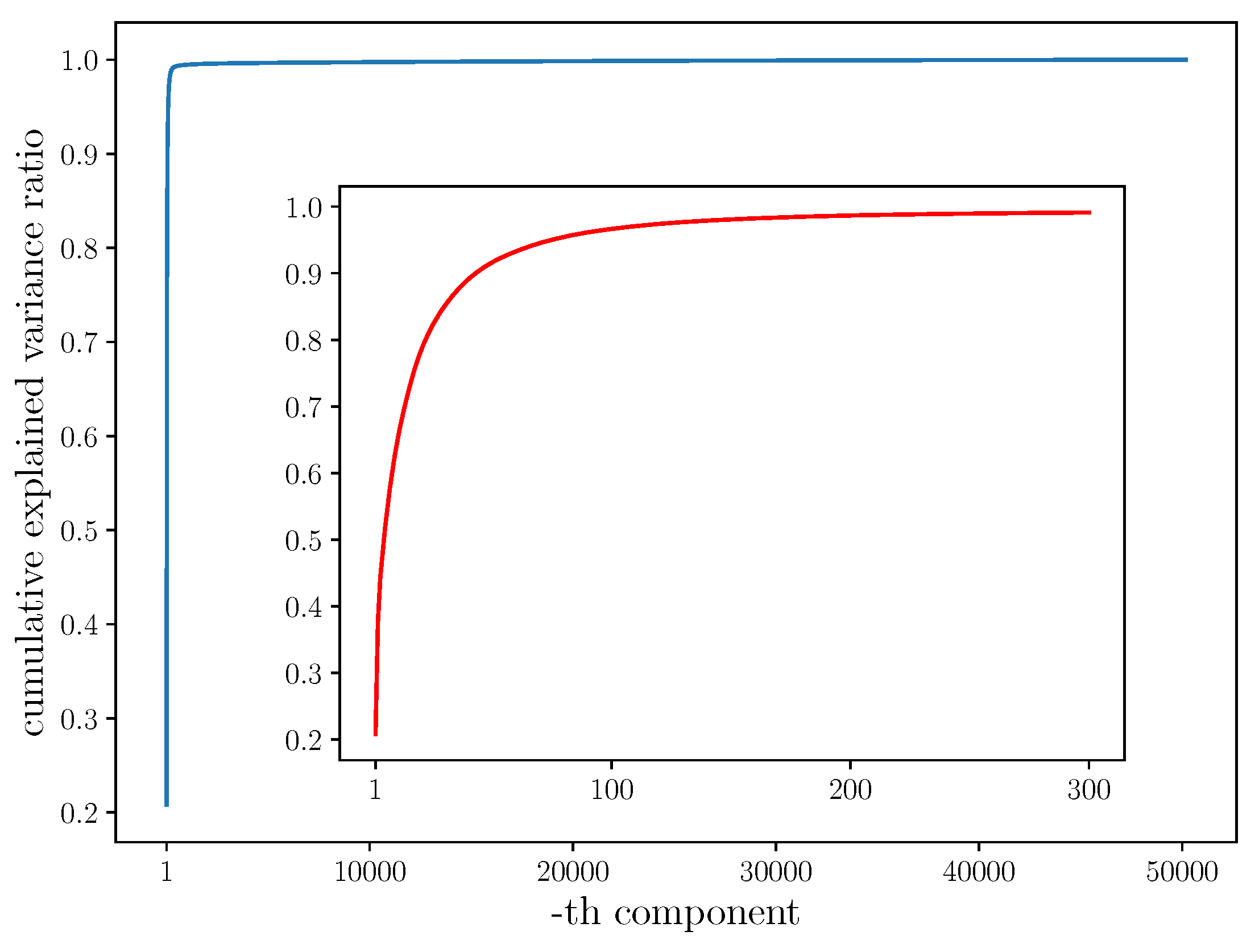
3.2. Analysis
4. Method
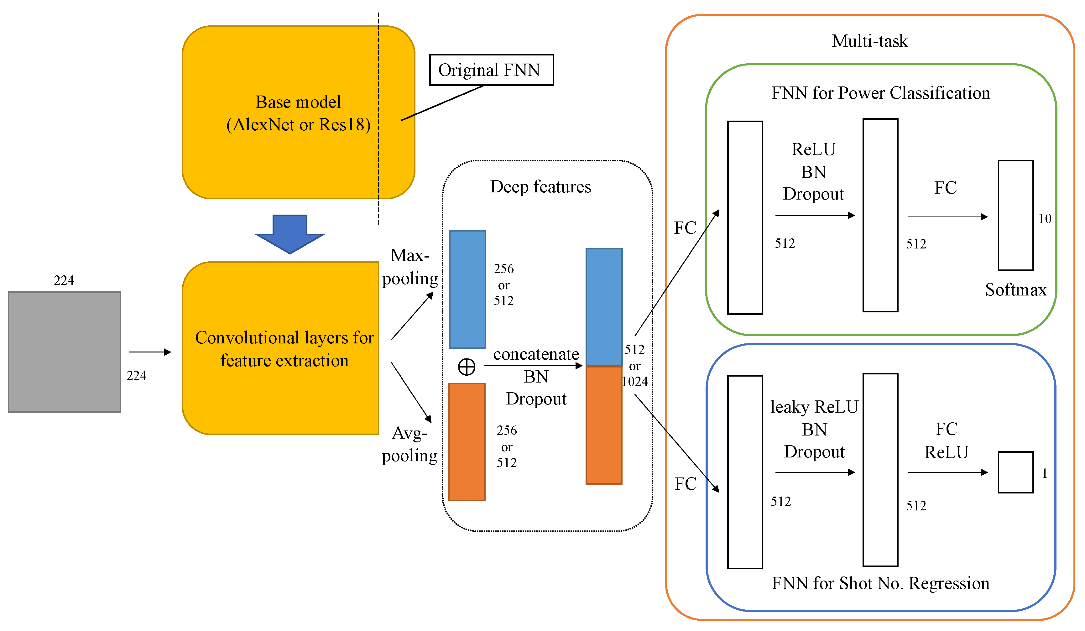
- Power Classification: Input an image, then predict the corresponding laser source power setting when this image was taken, i.e., classify the image to one of the 10 classes of laser power.
- Shot No. Regression: Input an image, then predict the logarithmic corresponding shot no. of this image, i.e., at which stage during a single experiment this image was taken, the shot no. can be one value in the range of 1–250.
4.1. Image Feature Extraction with CNN
- AlexNet [25] has five convolutional layers and three fully-connected (FC) layers and uses the rectified linear unit (ReLU) as the activation function instead of the sigmoid function to reduce gradient vanishing and gradient exploding problems. AlexNet also introduces mechanisms such as Dropout and overlapping pooling to avoid overfitting.
- ResNet [26] (Deep Residual Network) is designed for networks with great depths by introducing a new neural network layer, Residual Block, to alleviate the problem of training very deep networks. The most widely used variances of ResNet include Res18, which has 17 convolutional layers and one fully-connected layer.
4.2. Classification and Regression
4.3. Multi-Task Learning
5. Results and Discussions
5.1. Metrics and Settings
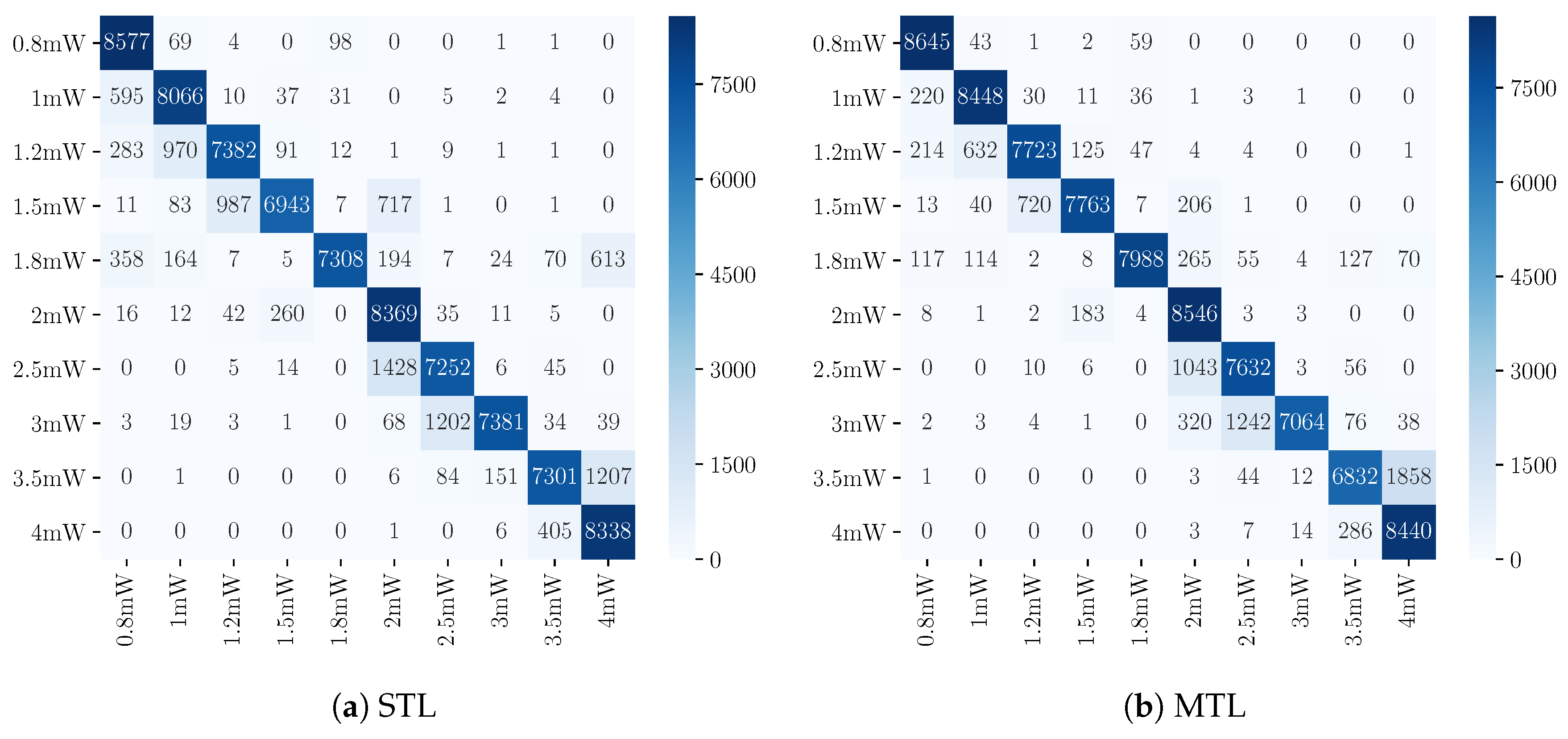
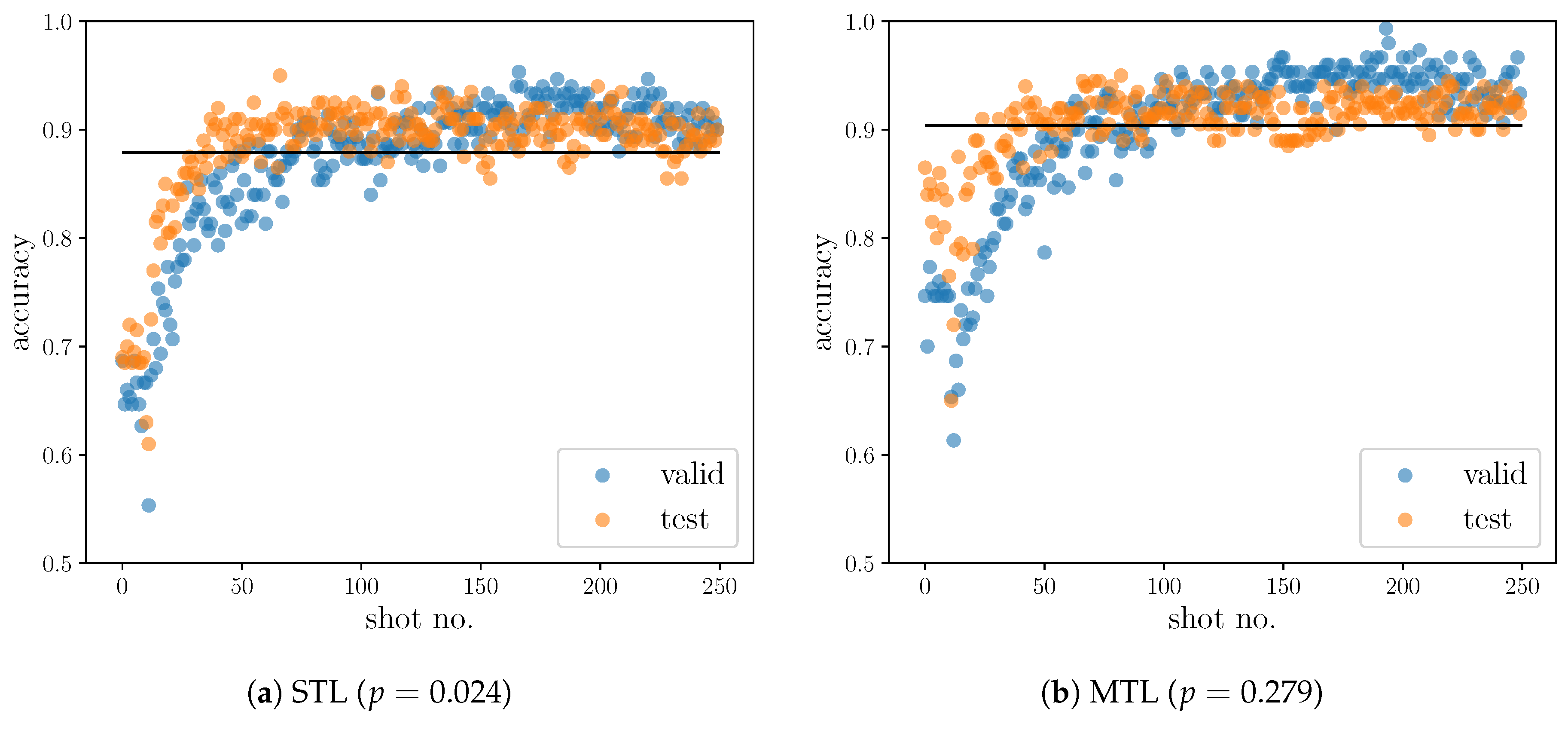
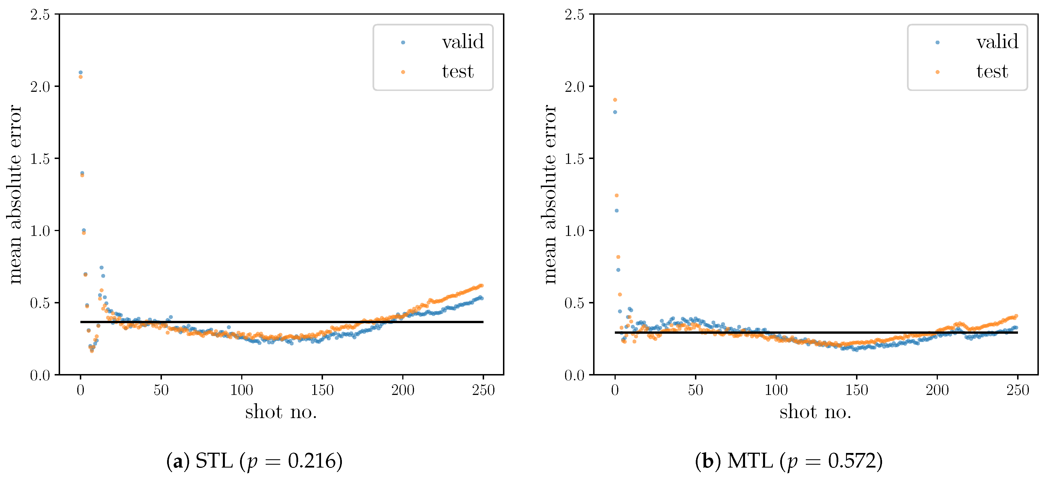
5.2. Results
6. Conclusions
Author Contributions
Funding
Acknowledgments
Conflicts of Interest
References
- Chryssolouris, G.; Stavropoulos, P.; Salonitis, K. Process of Laser Machining. In Handbook of Manufacturing Engineering and Technology; Nee, A., Ed.; Springer: London, UK, 2013. [Google Scholar]
- Tofail, S.A.; Koumoulos, E.P.; Bandyopadhyay, A.; Bose, S.; O’Donoghue, L.; Charitidis, C. Additive manufacturing: Scientific and technological challenges, market uptake and opportunities. Mater. Today 2018, 21, 22–37. [Google Scholar] [CrossRef]
- Shiner, B. The impact of fiber laser technology on the world wide material processing market. In CLEO: Applications and Technology; Optical Society of America: Washington, DC, USA, 2013; p. AF2J.1. [Google Scholar]
- Salgues, B. Society 5.0: Industry of the Future, Technologies, Methods and Tools; John Wiley & Sons: Hoboken, NJ, USA, 2018. [Google Scholar]
- Boyle, A.; Meighan, O.; Walsh, G.; Mah, K.W. Laser Machining System and Method. US Patent 7,887,712, 15 February 2011. [Google Scholar]
- Ohsawa, Y.; Kido, H.; Hayashi, T.; Liu, C.; Komoda, K. Innovators marketplace on data jackets, for valuating, sharing, and synthesizing data. In Knowledge-Based Information Systems in Practice; Springer: Berlin/Heidelberg, Germany, 2015; pp. 83–97. [Google Scholar]
- Ohsawa, Y.; Kido, H.; Hayashi, T.; Liu, C. Data jackets for synthesizing values in the market of data. Procedia Comput. Sci. 2013, 22, 709–716. [Google Scholar] [CrossRef]
- Ohsawa, Y.; Benson, N.E.; Yachida, M. KeyGraph: Automatic indexing by co-occurrence graph based on building construction metaphor. In Proceedings of the IEEE International Forum on Research and Technology Advances in Digital Libraries-ADL’98, Santa Barbara, CA, USA, 22–24 April 1998; pp. 12–18. [Google Scholar]
- Aoyagi, Y.; Tani, S.; Kobayashi, Y. Pulse-by-pulse measurement of ablation volume with deep learning. Jpn. Soc. Appl. Phys. 2017. [Google Scholar]
- Kobayashi, Y.; Tani, S. Automated data acquisition and deep learning in a laser processing. In JSAP-OSA Joint Symposia; Optical Society of America: Washington, DC, USA, 2018; p. 19p_231B_9. [Google Scholar]
- Tani, S.; Aoyagi, Y.; Kobayashi, Y. Neural-network-assisted in situ processing monitoring by speckle pattern observation. arXiv 2020, arXiv:2006.11351. [Google Scholar]
- Gatys, L.A.; Ecker, A.S.; Bethge, M. Image style transfer using convolutional neural networks. In Proceedings of the IEEE Conference on Computer Vision and Pattern Recognition, Las Vegas, NV, USA, 26 June–1 July 2016; pp. 2414–2423. [Google Scholar]
- Monteiro, R.; Bastos-Filho, C.; Cerrada, M.; Cabrera, D.; Sánchez, R.V. Convolutional neural networks using fourier transform spectrogram to classify the severity of gear tooth breakage. In Proceedings of the 2018 International Conference on Sensing, Diagnostics, Prognostics, and Control (SDPC), Xi’an, China, 15–17 August 2018; pp. 490–496. [Google Scholar]
- Mills, B.; Heath, D.J.; Grant-Jacob, J.A.; Xie, Y.; Eason, R.W. Image-based monitoring of femtosecond laser machining via a neural network. J. Phys. Photonics 2018, 1, 015008. [Google Scholar] [CrossRef]
- Zhang, Y.; Yang, Q. A Survey on Multi-Task Learning. arXiv 2017, arXiv:1707.08114. [Google Scholar]
- Collobert, R.; Weston, J. A unified architecture for natural language processing: Deep neural networks with multitask learning. In Proceedings of the 25th International Conference on MACHINE Learning, Helsinki, Finland, 5–9 July 2008; pp. 160–167. [Google Scholar]
- Deng, L.; Hinton, G.; Kingsbury, B. New types of deep neural network learning for speech recognition and related applications: An overview. In Proceedings of the 2013 IEEE International Conference on Acoustics, Speech and Signal Processing, Vancouver, BC, Canada, 26–30 May 2013; pp. 8599–8603. [Google Scholar]
- Ren, S.; He, K.; Girshick, R.; Sun, J. Faster r-cnn: Towards real-time object detection with region proposal networks. In Proceedings of the Advances in Neural Information Processing Systems, Montreal, QC, Canada, 7–12 December 2015; pp. 91–99. [Google Scholar]
- Ruder, S. An Overview of Multi-Task Learning in Deep Neural Networks. arXiv 2017, arXiv:1706.05098. [Google Scholar]
- Sener, O.; Koltun, V. Multi-task learning as multi-objective optimization. In Proceedings of the Advances in Neural Information Processing Systems, Montreal, QC, Canada, 3–8 December 2018; pp. 527–538. [Google Scholar]
- Evgeniou, T.; Pontil, M. Regularized multi–task learning. In Proceedings of the Tenth ACM SIGKDD International Conference on Knowledge Discovery and Data Mining, Seattle, WA, USA, 22–25 August 2004; pp. 109–117. [Google Scholar]
- Misra, I.; Shrivastava, A.; Gupta, A.; Hebert, M. Cross-stitch networks for multi-task learning. In Proceedings of the IEEE Conference on Computer Vision and Pattern Recognition, Las Vegas, NV, USA, 27–30 June 2016; pp. 3994–4003. [Google Scholar]
- Pearson, K. On lines and planes of closest fit to systems of points in space. Philos. Mag. 1901, 2, 559–572. [Google Scholar] [CrossRef]
- Hansen, P.C. The truncatedsvd as a method for regularization. BIT Numer. Math. 1987, 27, 534–553. [Google Scholar] [CrossRef]
- Krizhevsky, A.; Sutskever, I.; Hinton, G.E. Imagenet classification with deep convolutional neural networks. In Proceedings of the Advances in Neural Information Processing Systems, Lake Tahoe, NV, USA, 3–6 December 2012; pp. 1097–1105. [Google Scholar]
- He, K.; Zhang, X.; Ren, S.; Sun, J. Deep residual learning for image recognition. In Proceedings of the IEEE Conference on Computer Vision and Pattern Recognition, Las Vegas, NV, USA, 27–30 June 2016; pp. 770–778. [Google Scholar]
- Cortes, C.; Vapnik, V. Support-vector networks. Mach. Learn. 1995, 20, 273–297. [Google Scholar] [CrossRef]
- Paszke, A.; Gross, S.; Massa, F.; Lerer, A.; Bradbury, J.; Chanan, G.; Killeen, T.; Lin, Z.; Gimelshein, N.; Antiga, L.; et al. Pytorch: An imperative style, high-performance deep learning library. In Proceedings of the Advances in Neural Information Processing Systems, Vancouver, BC, Canada, 8–14 December 2019; pp. 8026–8037. [Google Scholar]
- Smith, L.N. Cyclical learning rates for training neural networks. In Proceedings of the 2017 IEEE Winter Conference on Applications of Computer Vision (WACV), Santa Rosa, CA, USA, 24–31 March 2017; pp. 464–472. [Google Scholar]
- Hendrycks, D.; Mazeika, M.; Kadavath, S.; Song, D. Using self-supervised learning can improve model robustness and uncertainty. In Proceedings of the Advances in Neural Information Processing Systems, Vancouver, BC, Canada, 8–14 December 2019; pp. 15637–15648. [Google Scholar]
- Bengio, Y.; Courville, A.; Vincent, P. Representation learning: A review and new perspectives. IEEE Trans. Pattern Anal. Mach. Intell. 2013, 35, 1798–1828. [Google Scholar] [CrossRef] [PubMed]


| Subset Name | Range of Experiment IDs | Total Number of Samples |
|---|---|---|
| Training | 1–70 | 175,000 |
| Validation | 71–85 | 37,500 |
| Test | 86–105 | 50,000 |
| Model | Validation | Test | ||||
|---|---|---|---|---|---|---|
| SVM with SVD | 0.44333 | 0.49753 | 0.43899 | 0.52022 | 0.53973 | 0.49488 |
| simple FNN | 0.71637 | 0.70822 | 0.71340 | 0.73178 | 0.77212 | 0.72773 |
| simple FNN with MTL | 0.71803 | 0.72773 | 0.70776 | 0.75502 | 0.78540 | 0.74073 |
| AlexNet | 0.87184 | 0.88112 | 0.87064 | 0.88446 | 0.89578 | 0.88406 |
| AlexNet with MTL | 0.90069 | 0.90809 | 0.90032 | 0.9061 | 0.91547 | 0.90524 |
| ResNet | 0.87912 | 0.89091 | 0.87580 | 0.89204 | 0.90394 | 0.89191 |
| ResNet with MTL | 0.85171 | 0.87135 | 0.85183 | 0.88202 | 0.89715 | 0.87770 |
| Model | Validation | Test | ||
|---|---|---|---|---|
| SVM with SVD | 0.83891 | –0.39754 | 0.83301 | –0.37363 |
| simple FNN | 0.40982 | 0.70053 | 0.41074 | 0.70823 |
| simple FNN with MTL | 0.42202 | 0.68666 | 0.41330 | 0.69938 |
| AlexNet | 0.35468 | 0.73977 | 0.37303 | 0.71816 |
| AlexNet with MTL | 0.28893 | 0.84342 | 0.29558 | 0.82798 |
| ResNet | 0.35415 | 0.76356 | 0.37520 | 0.76356 |
| ResNet with MTL | 0.32888 | 0.79420 | 0.34177 | 0.78346 |
© 2020 by the authors. Licensee MDPI, Basel, Switzerland. This article is an open access article distributed under the terms and conditions of the Creative Commons Attribution (CC BY) license (http://creativecommons.org/licenses/by/4.0/).
Share and Cite
Zhang, Q.; Wang, Z.; Wang, B.; Ohsawa, Y.; Hayashi, T. Feature Extraction of Laser Machining Data by Using Deep Multi-Task Learning. Information 2020, 11, 378. https://doi.org/10.3390/info11080378
Zhang Q, Wang Z, Wang B, Ohsawa Y, Hayashi T. Feature Extraction of Laser Machining Data by Using Deep Multi-Task Learning. Information. 2020; 11(8):378. https://doi.org/10.3390/info11080378
Chicago/Turabian StyleZhang, Quexuan, Zexuan Wang, Bin Wang, Yukio Ohsawa, and Teruaki Hayashi. 2020. "Feature Extraction of Laser Machining Data by Using Deep Multi-Task Learning" Information 11, no. 8: 378. https://doi.org/10.3390/info11080378
APA StyleZhang, Q., Wang, Z., Wang, B., Ohsawa, Y., & Hayashi, T. (2020). Feature Extraction of Laser Machining Data by Using Deep Multi-Task Learning. Information, 11(8), 378. https://doi.org/10.3390/info11080378