Article

Early Prediction of Quality Issues in Automotive Modern Industry

by
Reza Khoshkangini
1,*,
Peyman Sheikholharam Mashhadi
1,
Peter Berck
1,
Saeed Gholami Shahbandi
2,
Sepideh Pashami
1,
Sławomir Nowaczyk
1 and
Tobias Niklasson
3
1
Center for Applied Intelligent Systems Research (CAISR), Halmstad University, 30118 Halmstad, Sweden
2
Volvo Group, Connected Solutions, 40508 Göteborg, Sweden
3
Volvo Group, Q&CS, 40508 Göteborg, Sweden
*
Author to whom correspondence should be addressed.
Information 2020, 11(7), 354; https://doi.org/10.3390/info11070354
Submission received: 31 May 2020 / Revised: 17 June 2020 / Accepted: 29 June 2020 / Published: 6 July 2020

Abstract

:
Many industries today are struggling with early the identification of quality issues, given the shortening of product design cycles and the desire to decrease production costs, coupled with the customer requirement for high uptime. The vehicle industry is no exception, as breakdowns often lead to on-road stops and delays in delivery missions. In this paper we consider quality issues to be an unexpected increase in failure rates of a particular component; those are particularly problematic for the original equipment manufacturers (OEMs) since they lead to unplanned costs and can significantly affect brand value. We propose a new approach towards the early detection of quality issues using machine learning (ML) to forecast the failures of a given component across the large population of units. In this study, we combine the usage information of vehicles with the records of their failures. The former is continuously collected, as the usage statistics are transmitted over telematics connections. The latter is based on invoice and warranty information collected in the workshops. We compare two different ML approaches: the first is an auto-regression model of the failure ratios for vehicles based on past information, while the second is the aggregation of individual vehicle failure predictions based on their individual usage. We present experimental evaluations on the real data captured from heavy-duty trucks demonstrating how these two formulations have complementary strengths and weaknesses; in particular, they can outperform each other given different volumes of the data. The classification approach surpasses the regressor model whenever enough data is available, i.e., once the vehicles are in-service for a longer time. On the other hand, the regression shows better predictive performance with a smaller amount of data, i.e., for vehicles that have been deployed recently.

1. Introduction

Heavy-duty vehicles are complex systems with a vast number of possible specifications, in which component breakdowns can originate from multiple sub-components that malfunction for different reasons. However, in this day and age, such modern equipment logs large amounts of data using hundreds of sensors. This data can be potentially analyzed to provide early warnings about future quality issues. In this context, we are interested not only in the degradation of performance—e.g., decreased capacity of a battery due to heavy use or wear and tear, but also broken components—e.g., a compressor.
There are established lines of research on the prediction of components breakdowns, degradation, reliability, etc., in the context of the transportation and vehicle industry [1,2,3,4,5,6,7,8]. Recently, some of these studies provide fault detection systems under the umbrella of statistical machine learning approaches, such as deep neural networks, recurrent neural networks, and support vector machines [5,9,10,11]. They build diagnostic models based on the data, which are collected from machines to forecast the healthiness and unhealthiness of the machine or its components. Such forecasting is crucial, since manufacturers can potentially lower their maintenance costs significantly by identifying and remedying the quality problems before they happen for a considerable portion of the population. Such knowledge enables manufacturers to take the preventive actions in the short term and plan for the longer term. Even though the literature review shows significant progress in this area, there are few works focusing on quality issues detection and forecasting. The ones which focus on quality issue detection mostly relate warranty claims to the age of the vehicle or other machinery.
In this study, we take advantage of multiple sources of data consisting of a large number of parameters that capture status information about the vehicles over time. We use the data to forecast the ratio of component breakdowns for a population of vehicles produced within the same month, during the entire warranty period. In general, we aim to use the sensor data (logged vehicle data, LVD) and combine it with information collected on warranty claims (WCs). More specifically, this paper presents and compares two approaches: the first is predicting failure rate using historical information about the history of failure rates, through an auto-regressive model; the other maps out the usage information (LVD) into component failure probabilities for each truck separately, and aggregates these predictions during the entire period of interest.
Both approaches aim at predicting the failure rate over the vehicle population during the warranty period. The first approach uses regression to estimate the failure rate based on the operations of similar vehicles that have been in service before. It can take advantage of significantly more historical data and capture aspects such as seasonality; however, it is not able to account for possible design changes or manufacturing deficiencies that appear suddenly. The second approach uses a classification algorithm to predict components’ failures, based on the history accumulated from the particular population of interest. These predictions are aggregated and translated into the failure rate, and take into account specifics of usage and any potential early symptoms of unusual wear.
These two approaches are compared in the results section and provide a suggestion for manufacturers and workshops to assess which approach can be used for a reliable prediction under different conditions.
The classification algorithm consists of four stages as follows: stage 1 consists of data integration, where LVD and WC data are concatenated in a time series to be used as an input for the classification pipeline. The main purpose of this step is to label the LVD using claim information; stage 2 takes the place as a feature engineering process consisting pf feature selection to get the most informative sub-set of features, and feature extraction to generate new features from LVD to attain a valuable pattern that is conductive to a higher level of prediction performance; model construction as stage 3 is responsible to build several models based on the data collected from thousands of heavy duty trucks in different batches of productions. Finally, evaluation construction in stage 4 is in charge of assessing how the system performs in different batches of vehicle production over a year.
The rest of the paper is organized as follows. In Section 2, we review the related works in the field; then in Section 3 we describe the available data sources used in this work. Problem formulation and the proposed approach are described in Section 4 and Section 5, respectively. Section 6 describes the experimental evaluation and the results, which are followed by a discussion and conclusion of the work in Section 7.

2. Related Work

Diagnosing and identifying emerging issues and component failures enable the manufacturers to take preemptive action in the form of controlled handling of the necessary repairs and minimizing downtime for the customers. Most importantly, doing so allows the manufacturer to plan their maintenance strategy for the longer term. Under this hypothesis, numerous studies have been conducted over the past decades to develop various sorts of solutions in order for early prediction of components’ failures to minimize the quality issues [12,13,14]. In the same context, Kalman filter [15], time series and linear regression models have been used in order to build models to predict the number of warranty claims [16,17]. Another interesting forecasting method has been done in [18], wherein a mixed non-homogeneous Poisson process (NHPP) was used to predict the warranty claims. Within these studies, life time/age and mileage are mostly used as the two main factors to predict the quality issues. For example, Nozer et al. in [19] introduced a probabilistic model based on time, and a time-dependent quantity such as the amount of usage. Later, Chukova et al. in [20] exploited two variables, age and mileage, of the vehicle to estimate the mean cumulative number of claims. Similarly, using lifetime distribution, a warranty claim prediction model was provided by Kleyner et al. in [21] based on a piece-wise application of Weibull and exponential distributions. In general, this study contributes two main prediction tasks consisting of ongoing forecasting for the current products, and prediction of upcoming warranty at a product planning time. In [22,23], advantage was taken of artificial neural networks. For example, multi-layer perceptrons (MLP) [22,23], and radial basis [24] algorithms were exploited to predict quality issues. Similar techniques have been recently used to predict remaining useful lives (RULs) of the components [25,26,27,28,29]. As an example, in [25], an ANN model was developed by utilizing acoustic emission (AE) signals [30] to estimate the RULs of bearings in the gearbox. In [26], a similar ANN model for RUL prognostic is provided to estimate the RUL of bearings in wind turbine gearbox. Under this formulation—RUL—Benkedjouh et al. [31] proposed a diagnostic model, in which the isometric feature mapping reduction method and classical support vector machine were integrated, aiming to estimate the residual useful lives of bearings. Targeting the same component and problem to predict, Boskoski et al. in [32] introduced a RUL prognostic approach using Gaussian process (GP) models and Renyi-entropy-based features.
Manufacturers keep track of repairs and warranty claims in their customer service and quality assurance departments. Several studies have combined these statistics with the ages and lifetimes of particular components to estimate warranty claims in the future [33,34,35,36]. For instance, M.Y. You et al. in [37], combined the capability of classical statistical lifetime distribution preventive maintenance and predictive maintenance techniques for predicting residual life.
There do, however, exist several recent studies done in the automotive domain dealing with predictive maintenance [38,39,40], which take advantage of multiple available data-sources mentioned, and we think that the prediction of failures can be improved based on these developments. Taking all these studies into consideration, we hypothesize that prediction of quality concern (here we mean component failures, particularly component failure ratios) can be improved from the vehicles’ usage data during their operation and the history of reported failures over different seasons.

3. Data Presentation

In this section we present the two datasets, which were used to carry out the proposed forecasting method: Logged Vehicle Data (LVD), which basically includes usage and specification of the vehicles and is aggregated over time in a cumulative fashion; and Warranty Claim (WC) data, consisting of the claims’ information, as they are reported during the vehicles’ life time.

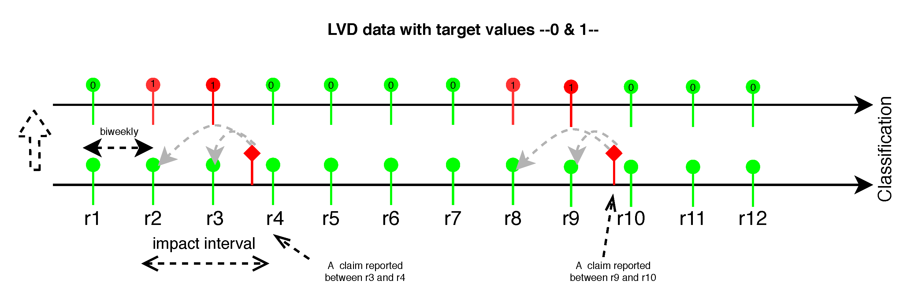
3.1. Logged Vehicle Data (LVD)

The logged vehicle data (LVD) used in this study were collected from commercial trucks over a three year period, from 2017 to 2019. The LVD consists of the aggregated usage information for a fleet of heavy-duty trucks operating in Europe. The values of the parameters were collected using telematics, and each time a vehicle visited an authorized workshop for repairs and service. In general, two types of parameters were logged in this dataset. The first type expresses the configuration of the vehicles; for example, the type of the engine, gearbox information, and the types of pumps. This information consists of categorical features. The second type logs the usage of the vehicle during its operation. These data are continuously aggregated and contain a number of different parameters, such as fuel consumption, compressor usage, gears used, cargo load, etc.

3.2. Claim Data

Claim data contain information regarding a vehicle’s warranty claims that were logged during its operation, collected by original equipment manufacturer (OEM)-authorized workshops in different places around the world. In particular, the claim database shows which part or component of which vehicle has been repaired or changed and on which date. The parts and components are defined by the normalized identification codes using four different levels of detail. For example, a single digit number can refer to all components related to the electrical system in a vehicle, whereas a four digit number (starting with that digit) refers to a specific component, such as the starter battery.
This claim dataset contains various parameters, such as vehicle ID, names of the components, codes and descriptions, dates, etc. It needs to be mentioned that in this study we only merged the parameters which are related to repaired date, component code and vehicle identification with the LVD from the claim dataset.

4. Problem Formulation

In this section, we present the two proposed formulations for failure ratio forecasting:
  • First we use only claim data, without LVD, to predict the future ratio of the vehicles’ failure over time, based on how it looked in the past. The approach is based on the assumption that the patterns of reported claims that happened in the past will also continue in the future.
  • Second, we have investigated the combination of the LVD and claim data, formulating it as a classification task to predict the failure ratio. Basically, the model acts based on the knowledge that can be extracted from vehicle usage to predict the upcoming failures. In this formulation, individual fault predictions are aggregated for the whole population into the failure ratio over time.
Concerning the above two formulations, we then define the ground truth failure ratio using Equation (1). The failure ratio F R G in the above formulations, can be calculated as the numbers of failures exploiting function I G ( i , t ) divided by the population of vehicles | V p | produced in that specific month | V p m | , which are operated and logged during a year.
F R G = i V p ( m ) t I G ( i , t ) | V p ( m ) |
I G ( i , t ) = 1 if vehicle i has failure in month t 0 else
These two formulations require two ML pipelines to be developed to provide a comprehensive forecasting solution. In the following sections we describe the proposed approach to tackle and answer the above formulations.

5. Approach

5.1. Approach 1: Forecasting Claim Rate Using Claim Data

The first approach in this study is based on claim data only. It basically regresses the past failure ratios against future failure ratios. Indeed, we hypothesize that the failures that happened in the past may provide a pattern that can be exploited to predict future possible failures. The goal is, first of all, is to identify how many past failures can be used to predict future failures. For the second: as the in-service time of vehicles increase, how much of this incremental information can help forecasting?
To investigate the first aspect, we regress the failure ratio during chosen months in-service against the remaining number of months in-service using a linear regression model. In particular, we take the advantage of a linear regression model, e.g., to predict failure ratio for the last nine months in-service from the first three months in-service.
To study the second aspect, we increase the in-service time, and at the same time, we predict the corresponding remaining in-service. In other words, we look at how much the prediction power will be increased as more information about failures is gathered.

5.2. Approach 2: Data Integration and Feature Engineering

Before diving into the second approach, a data preparation process for cleaning, selecting and extracting the most informative features need to be presented. The main two pre-processing components are data integration and feature engineering which are shown as Stage1 and Stage2 in Figure 1. The data integration and feature engineering processes are implemented on the two datasets.

5.2.1. Data Integration

The purpose of this module is to merge the LVD and claim datasets, to create an integrated dossier with both the usage and failure information for all the vehicles. We merge the two datasets based on the vehicle’s Chassis IF, date of readout and date of claim report. To this end, we select a time-window of one month preceding each warranty claim. We consider this to be the interval in which the symptoms of an imminent failure are most likely to be visible (indeed, we took advantage of expert knowledge to select this one-month time interval), and when the vehicle usage has the highest effect on a failure. An example of a one-month interval integration is illustrated in Figure 2, where the two closest readouts to the failure are marked as faulty samples.
The integrated dataset contains a new feature named failure (as the target feature f t ). This has a value of 1 for a given row if and only if a claim for the specific component of interest has been reported. More formally, each time-window/time span is assigned a binary label according to Equation (2), where t refers to a time window (one month) that has a highest impact on failures in trucks.
L t = 1 if failure in [ t , t + τ ) 0 if no failure in [ t , t + τ )

5.2.2. Feature Engineering

This module (initially developed in our previous study [40]) includes two sub-modules, feature selection and feature extraction, which are described as follows:

Feature Selection

Logged vehicle data (LVD), which were collected by multiple sensors in a time series, contain hundreds of parameters carrying valuable knowledge regarding vehicle usage style. However, we believe only a small subset of the data is informative for predicting component breakdowns. Thus, taking into account all the features F = { f 1 , f 2 , , f t } in the LVD, where f t is a target variable corresponding to the component breakdowns, we intend to pick a subset F s F of the features that are highly relevant for predicting the target value (healthy vs unhealthy vehicles). Due to the fact that every feature selection algorithm considers a different aspect of the data to select the most informative features, we exploit an ensemble method to select the features, where their importance can be seen from multiple algorithms. To this end, we used and integrated feature importance [41] and SelectKBest [42] algorithms in a parallel way (see [40]). (We have usedsklearn.feature_selection [43] library (Python) implementations of these feature selection algorithms.) Then, to obtain the desired list of features F s = { f 1 , f 2 , , f m , f t } , the common subset of features from the output of each algorithm is selected to build and train the model.

Feature Extraction

In contrast to the former process, where the intention was to decrease the dimensionality of the LVD, in this sub-module, we attempt to generate new features aiming to uncover the hidden information that can not be directly seen by feature selection algorithms. It has been recorded before, in a related study [44], that additional ways to represent data collected on-board vehicles can lead to increased classification performance.
In this module, we calculate the differences between subsequent data points, and exploit them as the new features in modeling. Figure 3a,b shows the examples of significant and moderate changes, highlighted in red and blue. These subplots show the changes in two different features (F1 and F2) in a vehicle (V1). The green line in both subplots shows the average movement in the changes during the vehicle’s operation.
We expect that the significant change (decrease or increase) in the vehicle’s usage pattern might be correlated with a failure in the near future. Figure 4a,b show how these changes are related to the healthy and non-healthy vehicles (healthy vehicles point to those that do not have any failures during their operational life, while unhealthy refers to the vehicles that have at least one reported breakdown in their history). In these two sub-figures, the y-axis shows the relative frequency of changes in four different categories. We have quantified the numbers of those changes and divided them into four categories; high, medium, low and no changes [45]. These are shown on the x-axis. These sub-figures clearly reveal that the proportion of significant positive and negative changes in non-healthy vehicles is higher than in the healthy vehicles during their lifetimes. In contrast, the proportion of healthy vehicles is more than that of non-healthy, when we took into consideration no changes to assess the correlation between them. Similar results were observed when medium and less significant changes were taken into consideration. Basically, the findings express the message that healthy vehicles have fewer usage deviations than unhealthy vehicles. Thus, this extra information may support the model to result in more accurate predictions.
We conducted this extraction on the list of the features ( F s ), which were obtained and selected from the Feature Selection module described in above. Thus, to construct the dataset to be trained by the classifiers in different experiments, we merged these extracted changes as extra parameters to the list F s , to get F s e = { f 0 s , f 1 s , f 2 s , , f m s , f 0 e x , f 1 e x , , f m e x } .

5.3. Approach 2: Forecasting Failure Rate Using LVD and Claim Data

This section presents our proposed approach in which forecasting is achieved based on the sensor data captured during vehicles’ operations. In this approach, we formulate the problem as the classification task exploiting the data logged from the vehicles (LVD), integrated with the claim data to predict the individual warranty claims/failures over time. We then aggregate all the individual predictions from the complete population into the failure ratio estimation. The conceptual view of the proposed classification method is illustrated in Figure 1, where in stage 3, the LVD is considered as vehicles behavior to predict the imminent failures during their warranty period. In this way, the vehicles which are produced in the same month (considered to be the same batch) are used to build the models for prediction task over time, and accordingly, to estimate the failure ratio of the complete batch of vehicles under their warranty period. Indeed, for every individual LVD sample, which shows the usage style of a particular vehicle in a certain time, we predict whether or not the vehicle will fail within a month, by taking into account the past usage and failures of the whole population of the vehicles produced in the same batch.
More to the point, in stage 3 (see Figure 5), we incrementally build multiple models such that the more time the vehicles are in service—e.g., one month, two months—the more LVD are considered for building the prediction model. In other words, we are incrementally adding more knowledge about vehicle usage in order to build the model to predict future failures until the end of their warranty time. Subsequently, over time, when the model exploits more LVD to train, the prediction time—here we mean the remaining time of warranty—will be decreased, since it reaches the end of the warranty period. For example, in the first iteration (e.g., for the first batch—Batch1 Figure 5—of our vehicles May-2017) we train the model with one-month vehicles LVD, and then the prediction process takes place with the data collected during the eleven months (from Jun-2017 to April-2018). In the second iteration—in this batch—the model uses two months of vehicle data in operation from May-2017 to June-2017 to be trained; accordingly, ten-months LVD from July-2017 to April-2018 are used for the validation part. These modeling and validation processes through different iterations continue until the end of the vehicles’ warranty periods. Over the year, different sorts of vehicles with various specifications have been produced in different months, so this way of modeling potentially supports the system to forecast any possible component breakdowns during the warranty period for each batch of vehicles.
Thus, given the failure ratio definition in Equation (1), we then formulate the prediction of failure ratio—in this classification pipeline—over time using Equation (3):
F R P = i V p ( m ) t I P ( i , t ) | V p ( m ) |
I P ( i , t ) = T P i , t + F P i , t 2
where T P i , t and F P i , t refer to the predicted failures of the vehicle i in month t . As it is described in the integration process, Section 5.2.1, and illustrated in Figure 2, we labeled two closest readouts/samples (in the LVD) as the faulty samples. Therefore, for each reported breakdown, we expect a “perfect” classifier to report two positive predictions. To account for that, we divide the sum of T P i , t + F P i , t by 2, to be comparable with ground truth F R G . Thus, as the predicted failure ratio, F R p , gets closer to the ground truth failure ratio, F R G , the model to predict the failure ratio in each production month becomes  more precise. In the next section, we describe in detail the evaluation of the two formulations by constructing various training and test sets over different vehicle production months.

6. Experimental Evaluation and Results

As it is explained in Section 1, the main objective of this study is failure ratio forecasting. Hence the goal of these experiments is to demonstrate to what extent we can predict components’ failure ratio during the vehicles’ warranty period based on their past claims and operation for every batch of vehicles. This provides valuable knowledge, so that an OEM can react if there is an increase in the claim/failure ratio under the warranty period. E.g., an increase in the failure ratio indicates that there is a quality problem in a specific component in a particular batch of vehicles. Thus, one should investigate more to avoid or decrease warranty claims before they happen. In this way, we illustrate how machine learning algorithms can be leveraged for failure prognostication taking into consideration the two data sources.
In this section, we present the evaluations and results of the two formulations to address the prediction task. In this task, we focus on the issue of predicting component failures for a particular component that is a part of power train, by building several models to forecast whether each individual vehicle will have a component failure within a month. The reason why multiple models are needed to be constructed is that we are predicting the failures for several different months. Thus, in this way, models gradually exploit more knowledge of vehicles’ usage (once they are more in-service) for building the models, and accordingly, the prediction in various months.
We used the Gradient Boosting (we took the advantage of sklearn library in Python to employ this classifier to build the model: https://scikit-learn.org/stable/modules/generated/sklearn.ensemble.GradientBoostingClassifier.html) algorithm to build the prediction models, where we constructed the training sets for the batches of vehicles produced in the same months over a year from May-2017 to April-2018. For each production month—e.g., the vehicles that are produced in May-2017; see Figure 5—we built eleven models so that the first model utilizes the data captured during one-month of the vehicles’ operation (here we assume the vehicles, e.g., with May-2017 production month, started to operate in the same month). Then, models incrementally exploit more knowledge once the vehicles are in the traffic more and more (e.g., two months, three months, etc.).
We first report how good the individual failure prediction models are across different production months. Figure 6 depicts the two ways of representation of auc values that we obtained as the prediction performance. Blue bars show the average of auc values, as obtained from eleven iterations for each production month. It can be observed that in most batches of vehicles auc values are above the random prediction > 0.50 . The lines show how the models perform with vehicles’ usage data with different numbers of months in operation. In fact, the lines—in different colors—represent the auc values obtained from the models, which are built based on LVD of the vehicles with different months in service/operation—such as three, five, eight and ten months—in each specific batch of production. It can be seen that, as expected, prediction based on 10-months in operation provides the best results a u c = 0.63 . However, in some cases, models based on eight months in operation perform better. Although the overall auc value achieved in this experiment is not a remarkable outcome, we should keep in mind that in this prediction task, we are dealing with a very difficult problem. Given the unbalanced data and the low informativeness of the collected signals, the performance of the predictive models on an individual vehicle is not expected to be high. Overall, the figures from experiments suggest that the more data that is collected (the longer vehicles are in-service) to model and map the vehicle usage to breakdowns, the better the predictions one can achieve are.
As it is shown in Equation (3), F R P represents the prediction of failure ratio in each production month, and the value of F R P is highly sensitive to the choice of the threshold on each confusion matrix (in other words, the values of TP and FP). To choose this threshold for each of the multiple models in every production month, we optimize F R P over a range of possible thresholds.
Figure 7 shows the average of the eleven optimal thresholds on failure ratio estimations and their standard deviations for each specific production month. Indeed, we aimed to find a static threshold so that we can utilize it for upcoming production months. Thus, we take the mean of all optimal thresholds achieved in each specific batch as the optimal threshold which is o p t = 0.53 . This optimal threshold can be used for the future data in which we do not have any ground truth to validate. Thus, to calculate the failure ratio, Equation (3) is used, where we obtained eleven different failure ratios for all batches of vehicles. For instance, if there are 20 faulty samples in the second iteration (in ten-months from Sept-2017 to Jun-2018) of the Batch3, in which 200 vehicles are produced, our model predicts 35, including TP and FP; so in this case the failure ratio would be (35/2)/200) = 0.0875. Indeed, this is a classification task by individual failure prediction, which translated to regression in the resulting level, where we measure the error between predicted failure ratios and ground truth failure ratios.
Figure 8 delineates the ground truth and the prediction of failures ratios, which are obtained by the two approaches. In fact, these are the resulting plots from the models constructed based on three, five, eight and ten-months of vehicles in operation. Accordingly, we considered both healthy and unhealthy samples, which are logged during the next nine, seven, four and two months to validate and estimate the failure ratio for all batch of vehicles. Since, in each production month, the failure population is distinct, the ground truths are different in each experiment, as depicted in Figure 8. For instance, the solid black lines show the actual failure ratios (actual numbers of failures divided by vehicles population in that batch) which happened during the vehicles operations, while the dash lines illustrate the prediction of failure ratios, from both approaches, under the warranty period.
As an example of the first approach, we train the model with eight months of operation, and then take the data, which were collected during four months, to forecast whether the vehicle will fail during the next month.
Concerning the results from classification approach, indeed it is expected to observe such poor performance with having less knowledge of vehicle usage; for instance, three or five months. The lack of this knowledge is more visible when we compare it with the result of regression approach. Figure 8 top three plots, green lines, clearly demonstrate how far the prediction using claim data is from the actual baseline—mostly from the vehicles, which are produced in 2017 with regard to the vehicles produced in 2018. In contrast, the red lines confirm the superiority of the regression using regression between failure ratio in the past to predict the failure ratios over all batches of vehicles, when three, five and eight months in operations are considered to build their models. This is reversed, however, once the classification approach gets enough usage knowledge to train the model. The bottom plot in Figure 8 depicts the overestimation of the failures ratios by the approach using only claims data; the classification performs better in all but one batches of vehicles.
Although we formulated this forecasting task as a classification problem by individual prediction of failures, once we considered the predicted numbers of breakdowns and translated to the failure ratio for each batch of vehicles, the problem is transformed into regression task in the result presentation level. Thus, to quantify and compare the performance of the two approaches, we calculated the mean absolute error (MAE) between ground truth and predicted ratios, which are reported in Table 1. Concerning the errors from the first approach, it could be observed the errors smoothly decreased from 0.25 to 0.12 considering three to ten months data, respectively, at building the models. The same trend was achieved by the classification approach, while we observed a significant drop in the errors; e.g., from three months (3.9) to five months (1.62) or from five and eight months (0.70) to ten months (0.08) once the model was trained by more data. Basically, they show to what extent more usage data is valuable to map the vehicle usage to component failures, so that classification formulation outperforms the regression model, once the model is trained with enough data. Overall, the figures depicted in the table confirm that the more data we get to build the models, the less error the models make to predict the upcoming failures.

7. Discussion and Conclusions

Two machine learning pipelines have been proposed in this study, for the early prediction of components’ failure ratio. This study found that estimating the ratios can be accomplished through vehicles’ usage patterns and failures history, whereas it did not receive much attention in the literature this way of addressing the problem. In these two pipelines, the prediction task is formulated as regression and classification problems, in which the evaluation of them has been constructed based on vehicles’ production dates, and their operations using two sources of data. We have (i) taken into account only claim data to calculate the regression between the previous failures and future failures to predict the upcoming breakdowns; (ii) taken into consideration vehicles’ usage with the integration of claim data (history of failures) to forecast failures, and then failure ratio over time.
For both formulations, the evaluation results show that the proposed solutions may support manufacturers in designing and scheduling their plan for the necessary actions—mainly in two situations. More to the point, the figures obtained from the two formulations suggest that the regression approach is suitable when the vehicles are less than ten months in-service. In contrast, the classification pipeline offers significantly better performance once well-enough data are available for building the prediction models. However, the low AUC and high MAE values obtained from the models throughout the evaluations signify that there still room to be improved in this way of tackling the prediction problem.
The findings of this work, however, have delivered limitations, which imply some new directions for our future research. The first limitation pertains to the issue of a very unbalanced data. In this work, the limited number of positive samples in the training set to build and draw inferences brings about a threat for validation, when we target a specific component, that should be addressed. Although we could observe an admissible result, in some batches of vehicles—see Figure 6—using special weight for the minority class to train the model, transfer learning [46] could be a solution [47]. The second limitation relates to the evaluation of the regression approach. It is fair to remark that, although our formulation and evaluation suggest how the correlation between the past failures could affect the failure ratio prediction over time, the evaluation constructed only based on reported failures so that if a failure is sourced from a poor design of vehicle, usage, etc., it is not be able to model them. The third limitation is associated with the components dependency and their influence to failure prediction and ratio. Our approach considers past failures, their correlations and LVD to forecast failures ratio over time; however, it does not include the parameters’ impact and relations to failures which is crucially important to recognize which can affect more to the ratio of failure over time.
An interesting extension of the solutions proposed in this study can be constructed aiming to address the third limitation described above. It is possible to conduct types of network dependencies [48] on top of LVD to extract the parameters dependencies and relations to breakdowns. These could reveal which parameters have the highest impact in failure ratio over time, so that enables the manufactures to properly plan their investigation on a specific component.

Author Contributions

Data curation, P.B., S.G.S., S.P., S.N. and T.N.; Formal analysis, P.S.M.; Supervision, R.K. All authors have read and agreed to the published version of the manuscript.

Funding

This research received no external funding.

Conflicts of Interest

The authors declare no conflict of interest.

References

  1. Pickett, A.K.; Pyttel, T.; Payen, F.; Lauro, F.; Petrinic, N.; Werner, H.; Christlein, J. Failure prediction for advanced crashworthiness of transportation vehicles. Int. J. Impact Eng. 2004, 30, 853–872. [Google Scholar] [CrossRef]
  2. Sobie, C.; Freitas, C.; Nicolai, M. Simulation-driven machine learning: Bearing fault classification. Mech. Syst. Signal Process. 2018, 99, 403–419. [Google Scholar] [CrossRef]
  3. Hirschmann, D.; Tissen, D.; Schroder, S.; De Doncker, R.W. Reliability prediction for inverters in hybrid electrical vehicles. IEEE Trans. Power Electron. 2007, 22, 2511–2517. [Google Scholar] [CrossRef]
  4. Fink, O.; Zio, E.; Weidmann, U. Predicting component reliability and level of degradation with complex-valued neural networks. Reliab. Eng. Syst. Saf. 2014, 121, 198–206. [Google Scholar] [CrossRef] [Green Version]
  5. Boss, G.J.; Jones, A.R.; Lingafelt, C.S.; McConnell, K.C.; Moore, J.E. Predicting Vehicular Failures Using Autonomous Collaborative Comparisons to Detect Anomalies. U.S. Patent 10,109,120, 6 July 2020. [Google Scholar]
  6. Yang, C.; Liu, J.; Zeng, Y.; Xie, G. Prediction of components degradation using support vector regression with optimized parameters. Energy Procedia 2017, 127, 284–290. [Google Scholar] [CrossRef]
  7. Ding, Z.; Zhou, Y.; Pu, G.; Zhou, M. Online failure prediction for railway transportation systems based on fuzzy rules and data analysis. IEEE Trans. Reliab. 2018, 67, 1143–1158. [Google Scholar] [CrossRef]
  8. Lei, Y.; Yang, B.; Jiang, X.; Jia, F.; Li, N.; Nandi, A.K. Applications of machine learning to machine fault diagnosis: A review and roadmap. Mech. Syst. Signal Process. 2020, 138, 106587. [Google Scholar] [CrossRef]
  9. Makridakis, S.; Spiliotis, E.; Assimakopoulos, V. Statistical and Machine Learning forecasting methods: Concerns and ways forward. PLoS ONE 2018, 13, e0194889. [Google Scholar] [CrossRef] [Green Version]
  10. Jegadeeshwaran, R.; Sugumaran, V. Fault diagnosis of automobile hydraulic brake system using statistical features and support vector machines. Mech. Syst. Signal Process. 2015, 52, 436–446. [Google Scholar] [CrossRef]
  11. Malhotra, R.; Jain, A. Fault prediction using statistical and machine learning methods for improving software quality. J. Inf. Process. Syst. 2012, 8, 241–262. [Google Scholar] [CrossRef] [Green Version]
  12. Kalbfleisch, J.; Lawless, J.; Robinson, J. Methods for the analysis and prediction of warranty claims. Technometrics 1991, 33, 273–285. [Google Scholar] [CrossRef]
  13. Kleyner, A.; Sanborn, K. Modelling automotive warranty claims with build-to-sale data uncertainty. Int. J. Reliab. Saf. 2008, 2, 179–189. [Google Scholar] [CrossRef]
  14. Corbu, D.; Chukova, S.; O’Sullivan, J. Product warranty: Modelling with 2D-renewal process. Int. J. Reliab. Saf. 2008, 2, 209–220. [Google Scholar] [CrossRef]
  15. Welch, G.; Bishop, G. An Introduction to the Kalman Filter; Technical Report; Advance Publication: Chapel Hill, NC, USA, 1995. [Google Scholar]
  16. Wasserman, G.S. An application of dynamic linear models for predicting warranty claims. Comput. Ind. Eng. 1992, 22, 37–47. [Google Scholar] [CrossRef]
  17. Chen, J.; Lynn, N.; Singpurwalla, N. Forecasting Warranty Claims; Advance Publication: Cranfield, UK, 1996. [Google Scholar]
  18. Fredette, M.; Lawless, J.F. Finite-horizon prediction of recurrent events, with application to forecasts of warranty claims. Technometrics 2007, 49, 66–80. [Google Scholar] [CrossRef]
  19. Singpurwalla, N.D.; Wilson, S.P. Failure models indexed by two scales. Adv. Appl. Probab. 1998, 30, 1058–1072. [Google Scholar] [CrossRef]
  20. Chukova, S.; Robinson, J. Estimating mean cumulative functions from truncated automotive warranty data. Mod. Stat. Math. Methods Reliab. 2005, 10, 121. [Google Scholar]
  21. Kleyner, A.; Sandborn, P. A warranty forecasting model based on piecewise statistical distributions and stochastic simulation. Reliab. Eng. Syst. Saf. 2005, 88, 207–214. [Google Scholar] [CrossRef]
  22. Wasserman, G.; Sudjianto, A. Neural networks for forecasting warranty claims. In Intelligent Engineering Systems Through Artificial Neural Networks; ASME Press: New York, NY, USA, 1996; pp. 901–906. [Google Scholar]
  23. Wasserman, G.S.; Sudjianto, A. A comparison of three strategies for forecasting warranty claims. IIE Trans. 1996, 28, 967–977. [Google Scholar] [CrossRef]
  24. Rai, B.; Singh, N. Forecasting warranty performance in the presence of the ‘maturing data’phenomenon. Int. J. Syst. Sci. 2005, 36, 381–394. [Google Scholar] [CrossRef]
  25. Elforjani, M.; Shanbr, S. Prognosis of bearing acoustic emission signals using supervised machine learning. IEEE Trans. Ind. Electron. 2017, 65, 5864–5871. [Google Scholar] [CrossRef] [Green Version]
  26. Teng, W.; Zhang, X.; Liu, Y.; Kusiak, A.; Ma, Z. Prognosis of the remaining useful life of bearings in a wind turbine gearbox. Energies 2017, 10, 32. [Google Scholar] [CrossRef] [Green Version]
  27. He, Y.; Han, X.; Gu, C.; Chen, Z. Cost-oriented predictive maintenance based on mission reliability state for cyber manufacturing systems. Adv. Mech. Eng. 2018, 10, 1687814017751467. [Google Scholar] [CrossRef] [Green Version]
  28. Louhichi, R.; Sallak, M.; Pelletan, J. A Cost Model for Predictive Maintenance Based on Risk-Assessment; Advance Publication: Paris, France, 2019. [Google Scholar]
  29. Ran, Y.; Zhou, X.; Lin, P.; Wen, Y.; Deng, R. A Survey of Predictive Maintenance: Systems, Purposes and Approaches. arXiv 2019, arXiv:1912.07383. [Google Scholar]
  30. Noorsuhada, M. An overview on fatigue damage assessment of reinforced concrete structures with the aid of acoustic emission technique. Constr. Build. Mater. 2016, 112, 424–439. [Google Scholar] [CrossRef]
  31. Remaining useful life estimation based on nonlinear feature reduction and support vector regression. Eng. Appl. Artif. Intell. 2013, 26, 1751–1760. [CrossRef]
  32. Bearing fault prognostics using Rényi entropy based features and Gaussian process models. Mech. Syst. Signal Process. 2015, 52–53, 327–337. [CrossRef]
  33. Kalbfleisch, J.; Lawless, J. Statistical analysis of warranty claims data. In Product Warranty Handbook; CRC Press: Boca Raton, FL, USA, 1996; pp. 231–259. [Google Scholar]
  34. Karim, R.; Suzuki, K. Analysis of warranty claim data: A literature review. In Advanced Reliability Modeling; World Scientific: Singapore, 2004; pp. 229–236. [Google Scholar]
  35. Lawless, J. Statistical analysis of product warranty data. Int. Stat. Rev. 1998, 66, 41–60. [Google Scholar] [CrossRef]
  36. Lei, Y.; Li, N.; Gontarz, S.; Lin, J.; Radkowski, S.; Dybala, J. A model-based method for remaining useful life prediction of machinery. IEEE Trans. Reliab. 2016, 65, 1314–1326. [Google Scholar] [CrossRef]
  37. You, M.Y.; Liu, F.; Wang, W.; Meng, G. Statistically planned and individually improved predictive maintenance management for continuously monitored degrading systems. IEEE Trans. Reliab. 2010, 59, 744–753. [Google Scholar] [CrossRef]
  38. Nowaczyk, S.; Prytz, R.; Rögnvaldsson, T.; Byttner, S. Towards a machine learning algorithm for predicting truck compressor failures using logged vehicle data. In Proceedings of the 12th Scandinavian Conference on Artificial Intelligence, Aalborg, Denmark, 20–22 November 2013; IOS Press: Amsterdam, The Netherlands, 2013; pp. 205–214. [Google Scholar]
  39. Prytz, R.; Nowaczyk, S.; Rögnvaldsson, T.; Byttner, S. Predicting the need for vehicle compressor repairs using maintenance records and logged vehicle data. Eng. Appl. Artif. Intell. 2015, 41, 139–150. [Google Scholar] [CrossRef] [Green Version]
  40. Khoshkangini, R.; Pashami, S.; Nowaczyk, S. Warranty Claim Rate Prediction Using Logged Vehicle Data. In EPIA Conference on Artificial Intelligence; Springer: Berlin, Germany, 2019; pp. 663–674. [Google Scholar]
  41. Behrens, T.; Zhu, A.X.; Schmidt, K.; Scholten, T. Multi-scale digital terrain analysis and feature selection for digital soil mapping. Geoderma 2010, 155, 175–185. [Google Scholar] [CrossRef]
  42. Yang, Y.; Pedersen, J.O. A comparative study on feature selection in text categorization. ICML 1997, 97, 35. [Google Scholar]
  43. Buitinck, L.; Louppe, G.; Blondel, M.; Pedregosa, F.; Mueller, A.; Grisel, O.; Niculae, V.; Prettenhofer, P.; Gramfort, A.; Grobler, J.; et al. API design for machine learning software: Experiences from the scikit-learn project. arXiv 2013, arXiv:1309.0238. [Google Scholar]
  44. Rögnvaldsson, T.; Nowaczyk, S.; Byttner, S.; Prytz, R.; Svensson, M. Self-monitoring for maintenance of vehicle fleets. Data Min. Knowl. Discov. 2018, 32, 344–384. [Google Scholar] [CrossRef]
  45. Khoshkangini, R.; Berck, P.; Gholami, S.; Pashami, S.; Nowaczyk, S. Prediction of Field Reliability Deviation from Logged Vehicle Data; Submitted ICDM; IEEE: Piscataway, NJ, USA, 2019. [Google Scholar]
  46. Pan, S.J.; Yang, Q. A survey on transfer learning. IEEE Trans. Knowl. Data Eng. 2009, 22, 1345–1359. [Google Scholar] [CrossRef]
  47. Schein, A.I.; Popescul, A.; Ungar, L.H.; Pennock, D.M. Methods and metrics for cold-start recommendations. In Proceedings of the 25th Annual International ACM SIGIR Conference On Research and Development in Information Retrieval, Tampere, Finland, 11–15 August 2002; ACM: New York, NY, USA, 2002; pp. 253–260. [Google Scholar]
  48. Hahn, P.R.; Murray, J.S.; Carvalho, C.M. Bayesian regression tree models for causal inference: Regularization, confounding, and heterogeneous effects. In Bayesian Analysis; Advance Publication: Staten Island, NY, USA, 2020. [Google Scholar]
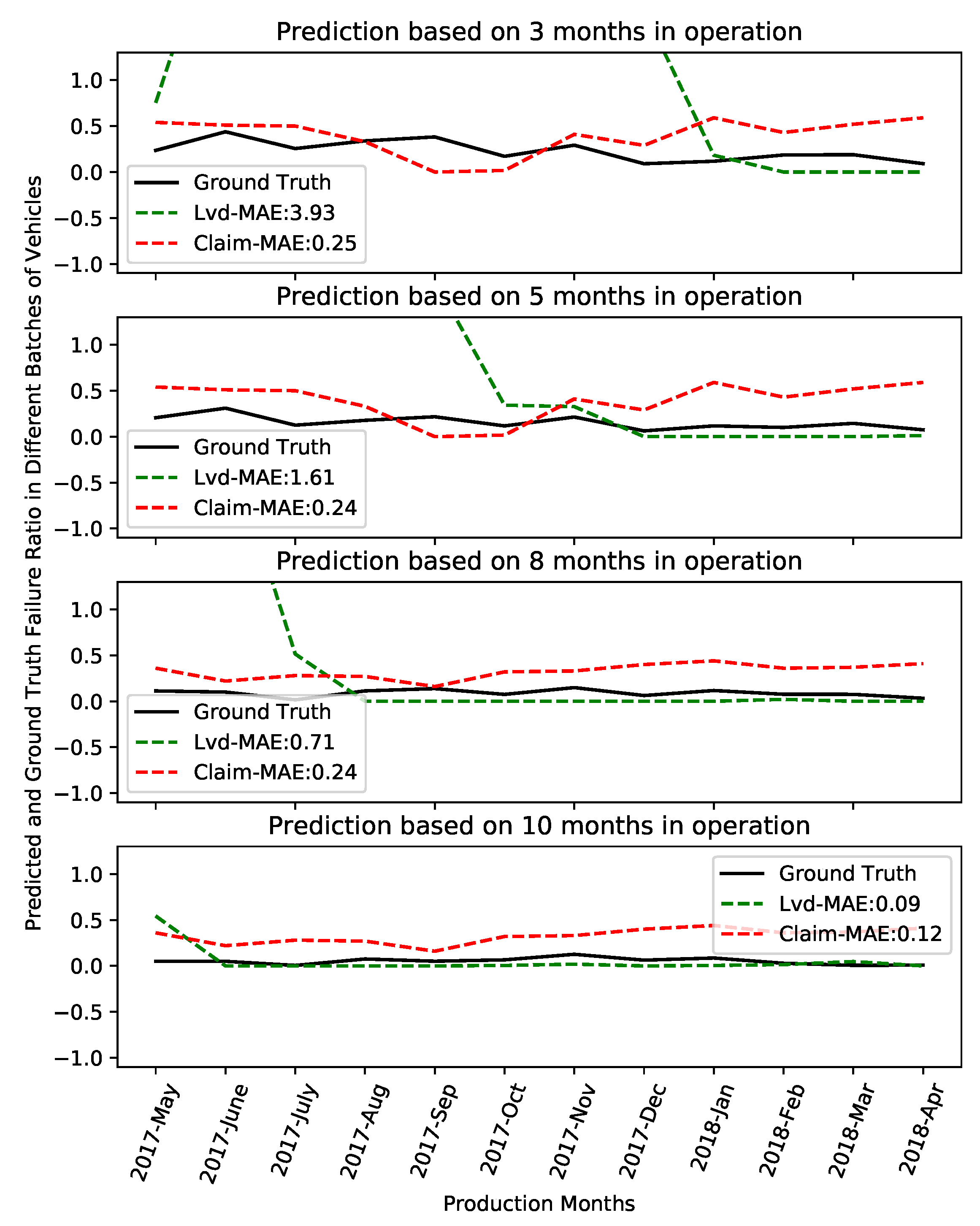
Figure 1. The conceptual view of the proposed classification method for predicting individual failures/claims with different pipelines.
Information 11 00354 g001
Figure 2. The conceptual view of labeling positive (non-healthy samples) and negative (healthy samples) target values in the logged vehicle data (LVD).
Information 11 00354 g002
Figure 3. Illustration of the extracted features distinguishing between significant and gradual changes in each feature. Subplots (a,b) show the changes in feature 1 (F1) and feature 2 (F2) in vehicle 1.
Information 11 00354 g003
Figure 4. Illustration of significant positive and negative usage changes in healthy and non-healthy vehicles. Subplots (a,b) show how the positive and negative significant usage changes, in one feature, relate to the health of the vehicles.
Information 11 00354 g004
Figure 5. The conceptual view of building and validating the model for all batches of vehicles produced in one year. This process incrementally increases the size of the training set by one month. Then the rest is considered to validate the model.
Information 11 00354 g005
Figure 6. AUC values in different production months.
Information 11 00354 g006
Figure 7. Mean values of eleventh optimal thresholds in different production months and the standard deviation of them, which were obtained from a range of possible thresholds in every iteration.
Information 11 00354 g007
Figure 8. Failure ratio in different vehicle production months.
Information 11 00354 g008
Table 1. Mean absolute errors of different predictions by the two approaches.
Three
Months
Five
Months
Eight
Months
Ten
Months
ClaimMAE0.250.240.240.12
LVDMAE3.91.610.700.08

