Article

Ensemble-Based Spam Detection in Smart Home IoT Devices Time Series Data Using Machine Learning Techniques

1
Electrical and Computer Engineering, Texas A&M University, College Station, TX 77843, USA
2
Electrical & Computer Engineering, Texas A&M University at Qatar, Doha 23874, Qatar
3
Research Computing, Texas A&M University at Qatar, Qatar Computing Research Institute, Hamad Bin Khalifa University, Doha 5825, Qatar
*
Author to whom correspondence should be addressed.
Information 2020, 11(7), 344; https://doi.org/10.3390/info11070344
Submission received: 1 June 2020 / Revised: 27 June 2020 / Accepted: 28 June 2020 / Published: 2 July 2020
(This article belongs to the Special Issue Machine Learning for Cyber-Physical Security)

Abstract

:
The number of Internet of Things (IoT) devices is growing at a fast pace in smart homes, producing large amounts of data, which are mostly transferred over wireless communication channels. However, various IoT devices are vulnerable to different threats, such as cyber-attacks, fluctuating network connections, leakage of information, etc. Statistical analysis and machine learning can play a vital role in detecting the anomalies in the data, which enhances the security level of the smart home IoT system which is the goal of this paper. This paper investigates the trustworthiness of the IoT devices sending house appliances’ readings, with the help of various parameters such as feature importance, root mean square error, hyper-parameter tuning, etc. A spamicity score was awarded to each of the IoT devices by the algorithm, based on the feature importance and the root mean square error score of the machine learning models to determine the trustworthiness of the device in the home network. A dataset publicly available for a smart home, along with weather conditions, is used for the methodology validation. The proposed algorithm is used to detect the spamicity score of the connected IoT devices in the network. The obtained results illustrate the efficacy of the proposed algorithm to analyze the time series data from the IoT devices for spam detection.

1. Introduction

Advanced metering infrastructure (AMI) is one of the most principal components of the smart grid, and it is comprised of hardware (smart meters) and software (data management systems and communication networks) components. AMI enables two-way communication between the utilities and the end customers. An AMI has structural similarities to a communication network; hence, techniques utilized in communication networks to combat privacy breaches, malicious activities, and monetary gain can be applied in the field of power grids [1]. The risk of the system infrastructure is higher than the risk of aggregated component elements. As the count of elements susceptible to attack increases in number, the system risk becomes more difficult and complex to trace [2]. Among the various types of smart grid threats, those concerning smart meters involve threats to network hub (poor isolation between meters power-line communication (PLC), and the smart meter’s outlet), distributor’s servers, link, management networks (user injecting frames supplanting the network hub identity), firmware updates, and hardware manipulation. In the case of the complete AMI, except for the displays, all the operations are vulnerable to alterations such as protocol design, network initialization, and key management and pose a threat to the AMI infrastructure. Threats interacting with the hardware to modify the memory are difficult to exploit. Meter tampering is one of the most obvious risks which appears in the form of adjusting the smart meter reading to send inaccurate information to the utility. This can result in inflated bills and providing wrong data for prediction and management which may result in severe consequences. The smart meters produce large amounts of data varied in terms of time and speed. Machine learning (ML) algorithms can be of noticeable importance to ensure the security of the smart home systems [3]. Injection of false data is a typical integrity attack and is a cyber-physical threat in modern smart grids. Automatic detection of faulty Internet of Things (IoT) devices was proposed with the help of context extraction [4]. A robust ensemble machine learning model was designed to detect the anomalies in the IoT devices based on the stored data [5]. The method proposed in [5] targets to detect anomalous events in smart home datasets with the help of ML model training. An analytical method was proposed to detect false data injection (FDI) by employing a margin setting algorithm in a data-centric paradigm [6]. Detection of an integrity attack such as false data injection (FDI) is possible with the help of analytical methods that utilize the smart grid’s huge amounts of data. Various methods were applied in the literature for the detection of anomalies in sensor data [5,7,8,9].
The addition of IoT devices to the smart home network adds challenges to the network elements such as communication, sheer amounts of data, storage, security, and privacy. Analysis of the data collected from the IoT devices can help in monitoring the energy consumption patterns and, in turn, control the energy consumption more efficiently [10]. The benefits of improving energy efficiency with the help of an AMI infrastructure is possible when the devices connected in the infrastructure are trustworthy. The adverse effects of receiving incorrect readings can lead to various issues and the energy management will tend to fail. The challenges faced in a smart home with IoT devices connected to the infrastructure include the lack of reliable and scalable cloud infrastructure platforms, ensured secure connections, information storage, and a lack of innovative products enabled with edge computing. A spam detection framework was proposed with the help of machine learning models to exploit the vulnerabilities in the smart IoT system [3].
This work is an extension of the work in [3], which assigns a spamicity score to the IoT devices. This work enhances the algorithm to deal with the time-series regression model instead of a classification model and can also execute ML models in parallel. This proposed paper focuses on determining the trustworthiness of the IoT device in the smart home network sending readings of the home appliances at a frequency of 1 min. The sensors’ readings were analyzed to find any anomalies by performing autocorrelation analysis. The algorithm scores an IoT device with a spamicity score to secure smart devices by detecting spam using different machine learning models. The main contributions of this paper can be summarized as below:
  • Analyzing the time-series data of the smart home IoT devices to understand the underlying structure of the data for better predictions.
  • Use of machine learning modeling to assign a feature importance score to the IoT device and predict the total consumption of energy.
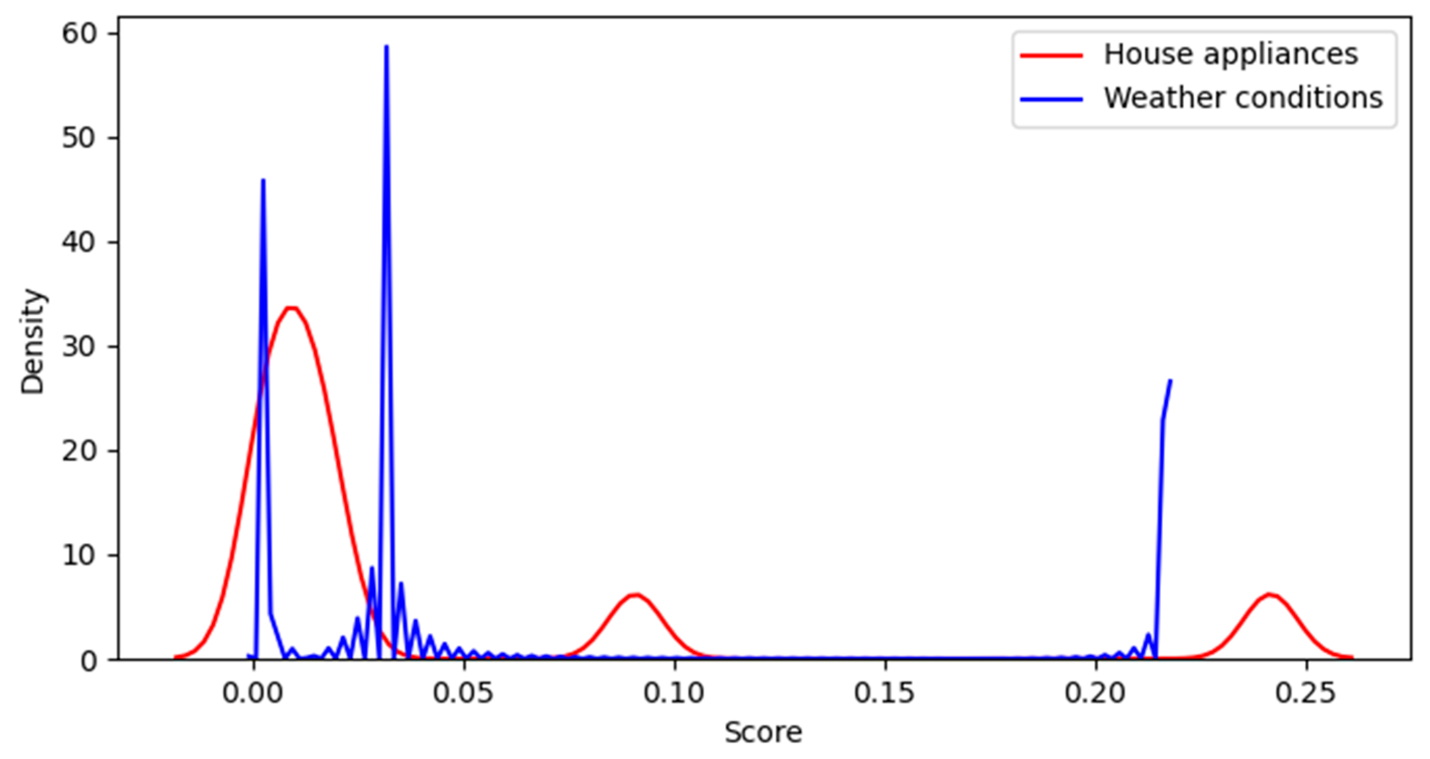
  • Calculation of a spam score of IoT devices to enhance the security of the smart home environment with the help of feature importance scores and the errors in energy prediction.
The remainder of this article is summarized as follows: Section 2 discusses the moving averages, followed by the machine learning models used in the analysis. The methodology of the algorithm used in the paper is also described in this section, followed by the spamicity measure statistic. Section 3 analyses the time series smart home data and discusses the data statistics and the results of calculating the spamicity score based on the algorithm described in Section 2. Section 4 concludes the paper.

2. Related Work

The home is a specific environment, and energy management is one of the IoT use cases with which energy being sent out or consumed can be monitored. One can monitor each of the IoT appliances and how much power each of the devices is consuming, and easily switch between energy-efficient appliances across the day. IoT security is a vital component to secure the IoT networks to protect against cybercrime. IoT devices indulge in huge data flows over high-speed internet resulting in challenges to control and manage the data flow. Artificial intelligence (AI) is claimed as one of the best solutions for data management and control in the IoT [11]. In the past few years, deep learning techniques have been explored and applied to the deluge of IoT devices [12]. Machine learning, a subset of AI, adds to the IoT revolution in the smart homes learning patterns of the appliances connected to the internet. An important motivation for the use of machine learning in the IoT security domain is to not rely on IP addresses of the devices which can be spoofed but the use of device data from the network. The field of cybersecurity utilized machine learning models for various applications such as keystroke dynamics, malicious URL detection, combating adversarial attacks, software vulnerability detection, automatic intrusion detection, spam email filtering, phishing URL detection, credit card fraud detection, capturing network traffic, Distributed Denial of Service (DDoS) detection, botnet traffic detection, etc. Ma et al. developed a framework by modeling the temporal sequence with the help of support vector regression for anomaly detection [13]. Each detection result generated based on the framework is designated with a confidence value. The authors worked on a variant of support vector regressor (SVR) which utilizes the Lagrange multipliers to calculate the weights of the models optimally. In the robust proposed online detection algorithm, the event duration n is chosen based on a voting procedure. The experiments were verified on both real data from a Santa Fe Institute competition with 1000-point time series and also synthetic data.
Several machine learning algorithms are used in the field of cybersecurity, broadly categorized into supervised and unsupervised approaches. One of the popular supervised learning examples is the detection of spam. Time series analysis and ensemble learning are two of the important concepts of machine learning. These concepts are utilized to analyze the historical data, compare them with the present, and detect any future deviations [14,15,16,17]. Makkar et al. developed a framework to detect web spam with the help of long short-term memory techniques [3]. The approach for spam classification in the IoT environment was also implemented in the research article to develop a framework for the Pagerank algorithm [18]. Wireless sensors can be vulnerable to attacks such as malicious injections creating fake events. Hau et al. proposed a framework to detect false data injections in heterogeneous sensor data to ensure data integrity in the IoT network [19]. A review article on the strengths and weaknesses of electrical power systems against malicious attacks has been discussed in [20]. Load altering attacks, data center attacks, and false command signals are some of the cyber-attacks provided by IoT.
The work emphasized in this paper distinguishes the good or bad network connections with the help of a spamicity score assigned to the IoT devices with the help of the algorithm. Various machine learning models aid the regression problem discussed in the paper to predict the time series load forecast. The related work emphasizes the fact that ML aids the detection of spam in the IoT devices by analyzing the time series data generated by the IoT devices.

3. Materials and Methods
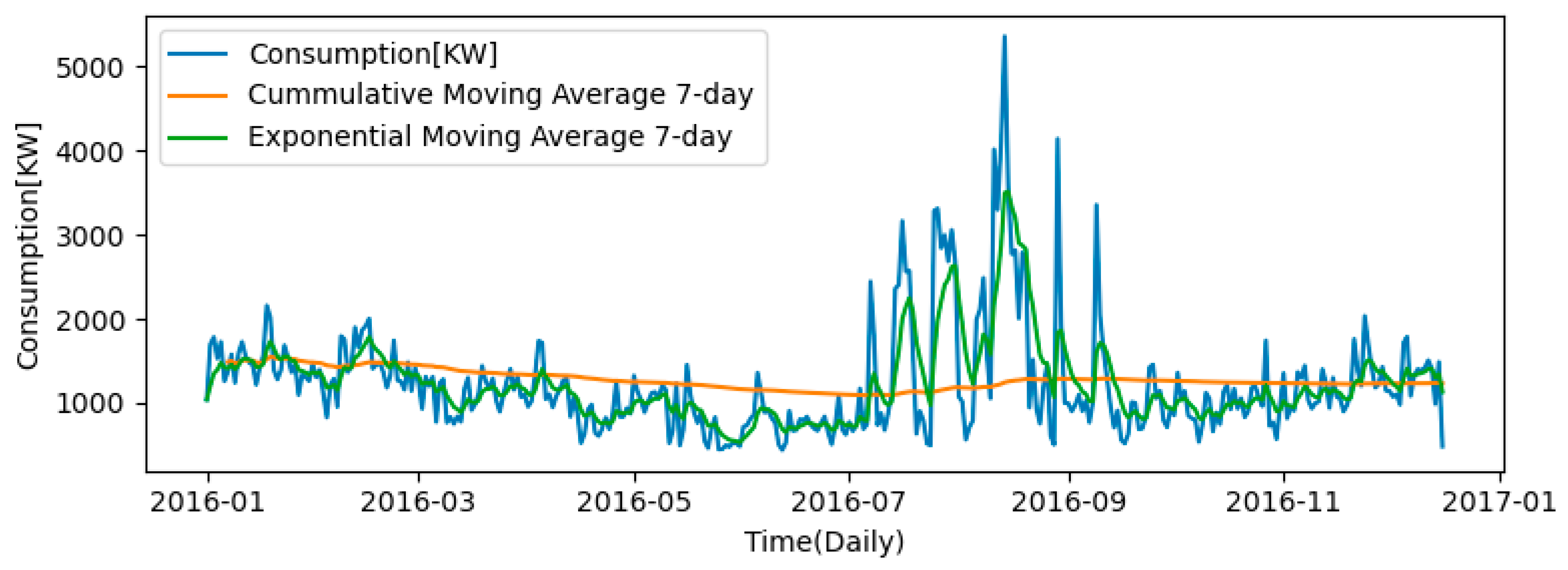
The use of machine learning models in the IoT has shown promising results for identifying malicious internet traffic using anomaly detection research [21]. Moreover, either detection of anomalies or the use of a spamicity score to track the security of the network components are motivated to have a safe and secure network infrastructure. For the energy sector, a secure AMI infrastructure plays an important role to enhance the overall security of the smart grids. In their paper, the authors discussed the prospects of bridging the gap between smart home devices and the IoT-enabled cloud-based environment [22]. Anomaly detection is an important step in the preprocessing data stages, as it helps in observing unexpected behavior. In [23], Bakar et al. discussed the importance of anomaly detection in the smart home environment as compared to other security domains. As the focus of this paper is to assign a spamicity score to the IoT devices, this section focuses on the data handling procedures, statistical insights, detection of anomalies in the data, and ML models used for the prediction, followed by the algorithm deployed to calculate the spamicity score.

3.1. Moving Average

Moving average forms, the basis of time series decomposition which is a commonly used technique to smooth out fluctuations in the data. Based on the timeframe, there are short-term and long-term moving averages which identify uptrend or downtrend of the data.
The easiest way to detect anomalies in time-series energy data is the use of moving averages as they capture the previous day’s trend. A data point that deviates from the moving average will be considered as an anomaly because the energy data do not expect a sudden rise and falls in the consumption values. There are various methods of calculating moving averages depending on the way the weight is added on the recent data points, such as:
  • Simple Moving Average (SMA)
This is an average of a series of data points over a given period. Moving averages are used to smooth out fluctuating data to identify overall trends and cycles. SMA is one the common averages and is the mean of the x data points, where each data point is weighted equally in the simple moving average, regardless of the occurrence the day before of x-1 days ago. The advantage of using an SMA is that it is straightforward and has a simple average price calculation. Depending on the type of application, the SMA might sometimes not be preferred due to the weight it gives to the old data and is not preferred for some of the applications.
  • Exponential Moving Average (EMA)
An EMA also takes an average of the data points over a given period; however, the weighting of each data point is not equal, as in the case of SMA. More weight is given to the recent data and the weighting is decreased as we go further back in time. EMA treats more recent data heavily as compared to the historical data.
E M A t = ( V t * α ) + E M A y * ( 1 α )
where α = s m o o t h i n g 1 + D ays , V t —value today and E M A y —previous EMA
Cumulative and exponential averages on the data set are presented in Figure 1. The data is resampled to a daily base using the sum to calculate the overall consumption in seven days. The benefit of EMA is that it is useful to identify recent trends. It is clear from the moving averages that the load consumption increased in the months of July, August, and September. However, the EMA signals are also more prone to identify false signals due to greater sensitivity.

3.2. Machine Learning Models

The proposed algorithm is validated with the help of four ML models summarized below to identify the spamicity score. Regression methods are widely used in the short-term and medium-term power forecasting fields [24]. Several ML models are utilized for supervised machine learning; however, this paper uses ensemble methods, a set of ML techniques based on decision trees. The machine learning models utilized in the paper are described in Table 1.
(1)
Extreme Gradient Boosting (XGBoost): This is a popular supervised machine learning model with characteristics of distributed and out-of-core computation, efficiency, and parallelization [25]. The parallelization occurs for multiple nodes in a single tree and not across trees. The complexity in XGboost is defined as:
Ω ( f ) = γ T + 1 2 λ j = 1 T w j 2
The term Ω penalizes the complexity of the regression tree functions. γ is a constant (a larger value of γ is associated with complex decision rules in which deeper nodes are penalized severely), w the weight, and T the number of leaves in a tree. The regularization added term helps in avoiding overfitting by smoothing the final learned weights. The main advantage of XGBoost is its scalability and quick execution speed, and it usually outperforms the other ML models [26].
(2)
Decision Trees: It employs a top-down approach, by utilizing standard deviation reduction to partition the data into subsets of homogeneous values [27]. It incorporates mixtures of categorical and numerical predictor variables with an integral part of the procedure to perform internal feature selection. These are the reasons why decision trees have emerged as one of the most popular data mining learning methods [28]. Decision trees can create an over-complex tree, which does not tend to generalize the data well and can result in overfitting. Even though the decision tree does not perform as well as neural networks for nonlinear networks, it is usually susceptible to noisy data. Decision trees expect visible trends in the data and also perform well on sequential patterns; if this is not the case, then decision trees have to be avoided for time series applications [29].
(3)
Random Forest: A supervised learning algorithm used for both classification and regression. It is an ensemble of decision trees which helps in reducing the variance in decision trees [30]. It performs a balance between high variance and high bias by sampling with each tree fitted and a sample of features at each split, respectively. The performance of random forest is dependent on the suitable selection of the number of trees, N. As in the case of bagging, a greater value of N does not necessarily overfit the data, and hence, a sufficiently large value of N can be chosen [31].
(4)
Gradient Boosted regression model: This model is like random forests, but the key difference is that the trees are built successively. The residual errors from the previous trees are fixed with the next tree to improve the fit [32]. One of the noticeable features of gradient boosted trees is that the algorithm detects the interactions among the features is detected automatically. However, the performance of gradient boosted trees is based on careful tuning and performs better than random forests if tuned appropriately. Gradient boosted trees are not preferred if the data consists of a lot of noise and can result in overfitting.
The four models discussed in Table 1 along with the parameters tuned are validated in Section 4.5. The R2 score and mean absolute error measure indicate the performance of the model;
  • a value closer to 100% indicates the model is highly correlated,
  • a value closer to 0 indicates the model to be perfect.

3.3. Methodology

The efficiency of an IoT device is determined by the efficiency of transmitting data by connecting wirelessly to the network. The efficiency increases if this data is stored, retrieved, and processed efficiently. The occurrence of spam in these devices is determined with the help of the error statistic spamicity score, as discussed in Section 3.4. The occurrence of spam is reduced by utilizing Equation (1).
m i n ( S ) = I s
where I indicates data collected, and s indicates the data related to spam. The lower the value of S , the better the chances of collecting data for IoT devices free of spam.
The model is divided into two main steps of finding the feature weights and the choice of the ML model. The flow chart in Figure 2 illustrates the methodology used in this paper. The flow chart has three stages. Stage 1 involves the choice of ML model parameters for the prediction of energy consumption using the R-squared (R2) statistical method. Each ML model with the best parameter is used to predict the power consumption and to calculate the RMSE score. Stage 2 involves the scoring of features based on the relative importance score of each of the input features. Stage 3 calculates the spamicity score from the results in Stage 1 and Stage 2. The regression tree algorithm is used to measure the feature importance, summarizing the calculated feature importance scores illustrated in Table 2. The importance of the features’ array sums to 1 and is derived as the normalized total reduction of the Gini criterion.

3.4. Spamicity Score

The validation of the proposed method is measured with the help of the spamicity score [3]. The spamicity score measures the trustworthiness and reliability of the IoT device. The spamicity score of each of the IoT devices connected in the network is measured by the equation below.
R M S E [ i ] = 1 n i = 1 n ( y i y P ) 2
S R M S E [ i ] * F i
where y i   and   y P are the actual and predicted values, n is the number of samples, R M S E [ i ] is the error sample of each feature, F i is the feature importance vector, and S is the spamicity score of each of the IoT devices. The spamicity score is calculated as a product of the error rate and the feature importance score. The complete procedure of calculating the spamicity score is iterated in Algorithm 1. The Spamicity score of all the devices is tabulated in Table 6.
Algorithm 1Calculation of Spamicity Score
InputTime series data
OutputSpamicity score
f <- Features (data)
Target <- data
Model (Features, target)      Choice of ML model
importance <- model(feature importances)
for i, v
F i <- enumerate(importance)    calculating the feature scores
end for
params <- {p1, p2, p3}
for i in params
 model (params)
 R2 score [i]        R2[i]= 1 first   sum   of   errors second   sum   of   errors
 best parameter <- result
end for
def MLpool(i)
for m = 1 to count(Mi) do
  model(best parameter)
  RMSE[i]      RMSE[i]= 1 n i 1 n ( y i y p ) 2
end for
w <- workers
p <- pool(w)p (MLpool, f)
end def
for j = 1 to count(f) do S ⇐ R M S E [ i ] * F i
end for

4. Results

4.1. Data Description

A public dataset of smart home IoT devices with weather features was utilized in this paper to perform the experiments [33]. The dataset ranges from 2016-01-01 08:00:00 to 2016-12-31 23:00:00 at a frequency of 1 min. The data statistic of power consumption [kW] is described below. Table 3 summarizes the dataset considered for the analysis. It helps us understand the variability (spread) of the data. The mean is close to 1, which determines the estimate of the value of the complete dataset. The standard deviation is also close to 1 and shows the average distance of the data points from the mean.
The data includes the following appliances: Dishwasher’, ‘Home office’, ‘Fridge’, ‘Wine cellar’, ‘Garage door’, ‘Barn’, ‘Well’, ‘Microwave’, ‘Living room’, and ‘Solar’ and weather features as indicated in Figure 3. It consists of smart home devices along with the weather information of the IoT devices in the smart home network.
The power consumption patterns of the monthly resampled data indicated in Figure 4 illustrate that the home office has the highest consumption and microwave has the lowest consumption. The wine cellar shows a peak in September. The garage door also shows low energy consumption levels. The home appliances such as microwave oven, garage door, and dishwasher, which are directly linked to the human movements irrespective of the weather, show almost constant energy consumption patterns.

4.2. Feature Selection

The feature selection is the first step to reduce the complexity of the model and to understand the effect of the features on the overall energy prediction patterns.
Feature selection is the method of choosing the best subset of features by computing the significance of each one of the features in the dataset [31]. Machine learning modeling also helps in assigning a feature importance score to each of the features. Every machine learning model utilized to fit the data is also used to evaluate its feature importance score. Table 2 lists the feature importance score of all the features using regression trees.

4.3. Data Preprocessing

An important step in the process is to make sure that the data is complete and satisfies all the requirements for data analysis. Any preprocessing step performed must be implemented vigilantly to avoid corruption in the dataset. Missing values were replaced with the next valid observation. The dataset was resampled to daily and monthly datasets based on the analysis requirements. Figure 5 is the autocorrelation plot of the data resampled to a monthly base. A value k is chosen based on the time gap considered in the time series to understand the linear relationship between an observation at the time t and its value at previous times. It can be depicted from Figure 5 that there is a strong correlation at the early lag days, but this tends to decay near the lag variable value of 12 days.

4.4. Data Statistics

A combination of approaches, such as subtracting from the mean, differencing, log transformation, measuring percentage change, etc., may be conducted to deserialize or detrend a time series. The density of the observations shown in Figure 6 provides insights into the structure of the data by providing data visualization over a continuous interval of time. The distribution is not suggested to be a Gaussian distribution; the right long line suggests the observation to be an exponential distribution due to a peak and exponentially decreasing values.
Autocorrelation determines the similarity between the observations as a function of time lag by performing a serial correlation of a time-domain signal with itself as a function of delay. The peaks in the autocorrelation help in determining the anomalies/noise in the data. Figure 5 indicates the autocorrelation of consumption.
The blue shaded region is the margin of uncertainty of the average of measurements and sticks extending beyond the blue region are considered statistically significant to not have occurred by chance.
Time-series data set can be stationary and non-stationary. Before applying any analysis, data is expected to be stationary, because a lot of analytical tools depend on it and expect the time series to not change drastically over time. The augmented Dickey–Fuller (ADF) test has been utilized to test the stationarity of the data, which claims as the null hypothesis that the data is non-stationary due to the trend [34]. When the null hypothesis is rejected, we can claim that the time series is stationary. The first difference (data at time t - data at time t-1) of the data is considered for the calculation of the ADF analysis.
Referring to Table 4. the value of p is 0.0, which is less than the threshold of 0.05, and the absolute value of the test statistic exceeds the absolute value of the 5% critical value. Hence, the null hypothesis can be rejected, claiming that the p-value is statistically significant, and the series data can be claimed to be stationary.

4.5. Results of Machine Learning Models on the Smart Home Dataset

In Figure 7, orange indicates the projections of the test dataset and the blue the prediction on the training dataset. The values show visually how good or bad the model is. The dataset was trained on the four ML models discussed in Section 3.2, and the results are depicted in Table 5 below. It provides a summary of the performance of the four machine learning models used in the experiments. The results in Table 6; Table 7 illustrate the spamicity score of the IoT devices and the weather features, respectively. The distribution of the spamicity scores of all four ML models is presented in Figure 8, Figure 9, Figure 10 and Figure 11. The evaluation was done using the R2 score test to choose the ML model and the feature importance score of all the features under consideration. The spamicity score is a product of two numbers, RMSE and the feature importance. An RMSE score cannot be considered good or bad, but surely a lesser value is always preferred. In the case of feature importance, a value closer to 1 is preferred, as the greater the number, the more important the feature is. It is not easy to define a threshold, but a score value in the range of e−3 can be considered as spam, as the values it records are of very low importance and also do not help in predicting the power consumption. The spikes in Figure 8, Figure 9, Figure 10 and Figure 11 in the vicinity of 0 indicate the occurrence of spam in the data collected from both the IoT devices and the weather features.

5. Conclusions

Efficient spam detection in the IoT devices has drawn significant attention from researchers, developers of the industries, and academics in recent years. This paper determines the use of the spamicity score to understand the trustworthiness of IoT devices in the smart home network. The proposed algorithm is used to determine the spam score of all IoT devices. Through rigorous tests and experiments, various ML models were utilized to analyze the time-series data generated from smart meters. Various contribution levels of the IoT devices were determined with the help of ensemble methods of machine learning by awarding a spam score to the IoT devices in a smart home. The results show that the spamicity score of the devices helps in refining the conditions of the successful IoT device functioning in the smart home.
The provided data from the smart home, along with the weather features, can be effectively utilized to award a spam score and can help in determining the security of the IoT devices.

Author Contributions

Data Curation, A.Z.; Conceptualization, A.Z. and O.B.; Formal analysis, A.Z.; Validation, S.S.R. and O.B.; Software, A.Z.; Supervision, S.S.R; Writing–Original draft, A.Z.; Review–Editing, S.S.R. and O.B. All authors have read and agreed to the published version of the manuscript.

Funding

This research was funded by Qatar National Research Fund grant number [NPRP10-0101-170082].

Acknowledgments

This publication was made possible by the NPRP grant [NPRP10-0101-170082] from the Qatar National Research Fund (a member of Qatar Foundation) and the co-funding by IBERDROLA QSTPLLC. The findings achieved herein are solely the responsibility of the author[s].

Conflicts of Interest

The authors declare no conflicts of interest.

References

  1. Chapter 19: Admission Control-Based Load Protection in the Smart Grid—Security and Privacy in Cyber-Physical Systems. Available online: https://learning.oreilly.com/library/view/security-and-privacy/9781119226048/c19.xhtml (accessed on 30 April 2020).
  2. Smart Meters—Threats and Attacks to PRIME Meters—Tarlogic Security—Cyber Security and Ethical Hacking. Available online: https://www.tarlogic.com/en/blog/smart-meters-threats-and-attacks-to-prime-meters/ (accessed on 5 May 2020).
  3. Makkar, A.; Garg, S.; Kumar, N.; Hossain, M.S.; Ghoneim, A.; Alrashoud, M. An Efficient Spam Detection Technique for IoT Devices using Machine Learning. IEEE Trans. Ind. Inform. 2020. [Google Scholar] [CrossRef]
  4. Choi, J.; Jeoung, H.; Kim, J.; Ko, Y.; Jung, W.; Kim, H.; Kim, J. Detecting and identifying faulty IoT devices in smart home with context extraction. In Proceedings of the 48th Annual IEEE/IFIP International Conference on Dependable Systems and Networks, DSN 2018, Luxembourg, 25–28 June 2018; pp. 610–621. [Google Scholar] [CrossRef]
  5. Tang, S.; Gu, Z.; Yang, Q.; Fu, S. Smart Home IoT Anomaly Detection based on Ensemble Model Learning from Heterogeneous Data. In Proceedings of the 2019 IEEE International Conference on Big Data (Big Data), Los Angeles, CA, USA, 9–12 December 2019; pp. 4185–4190. [Google Scholar] [CrossRef]
  6. Wang, Y.; Amin, M.M.; Fu, J.; Moussa, H.B. A novel data analytical approach for false data injection cyber-physical attack mitigation in smart grids. IEEE Access 2017, 5, 26022–26033. [Google Scholar] [CrossRef]
  7. Alagha, A.; Singh, S.; Mizouni, R.; Ouali, A.; Otrok, H. Data-Driven Dynamic Active Node Selection for Event Localization in IoT Applications—A Case Study of Radiation Localization. IEEE Access 2019, 7, 16168–16183. [Google Scholar] [CrossRef]
  8. Mishra, P.; Gudla, S.K.; ShanBhag, A.D.; Bose, J. Enhanced Alternate Action Recommender System Using Recurrent Patterns and Fault Detection System for Smart Home Users. In Proceedings of the 2019 IEEE International Conference on Big Data (Big Data), Los Angeles, CA, USA, 9–12 December 2019; pp. 651–656. [Google Scholar] [CrossRef]
  9. Gaddam, A.; Wilkin, T.; Angelova, M. Anomaly detection models for detecting sensor faults and outliers in the iot-a survey. In Proceedings of the 2019 13th International Conference on Sensing Technology (ICST), Sydney, Australia, 2–4 December 2019. [Google Scholar] [CrossRef]
  10. Motlagh, N.H.; Khajavi, S.H.; Jaribion, A.; Holmstrom, J. An IoT-based automation system for older homes: A use case for lighting system. In Proceedings of the 2018 IEEE 11th Conference on Service-Oriented Computing and Applications (SOCA), Paris, France, 20–22 November 2018; pp. 247–252. [Google Scholar] [CrossRef]
  11. Osuwa, A.A.; Ekhoragbon, E.B.; Fat, L.T. Application of artificial intelligence in Internet of Things. In Proceedings of the 9th International Conference on Computational Intelligence and Communication Networks, CICN 2017, Girne, Cyprus, 16–17 September 2017; pp. 169–173. [Google Scholar] [CrossRef]
  12. Song, M.; Zhong, K.; Zhang, J.; Hu, Y.; Liu, D.; Zhang, W.; Wang, J.; Li, T. In-Situ AI: Towards Autonomous and Incremental Deep Learning for IoT Systems. In Proceedings of the 2018 IEEE International Symposium on High Performance Computer Architecture (HPCA), Vienna, Austria, 24–28 February 2018; pp. 92–103. [Google Scholar] [CrossRef]
  13. Ma, J.; Perkins, S. Online novelty detection on temporal sequences. In Proceedings of the ACM SIGKDD International Conference on Knowledge Discovery and Data Mining, Washington, DC, USA, 24–27 August 2003; pp. 613–618. [Google Scholar] [CrossRef]
  14. Li, J.; Pedrycz, W.; Jamal, I. Multivariate time series anomaly detection: A framework of Hidden Markov Models. Appl. Soft Comput. J. 2017, 60, 229–240. [Google Scholar] [CrossRef]
  15. Flanagan, K.; Fallon, E.; Connolly, P.; Awad, A. Network anomaly detection in time series using distance based outlier detection with cluster density analysis. In Proceedings of the 2017 Internet Technologies and Applications (ITA), Wrexham, UK, 12–15 September 2017; pp. 116–121. [Google Scholar] [CrossRef]
  16. Zhang, A.; Song, S.; Wang, J.; Yu, P.S. Time series data cleaning: From anomaly detection to anomaly repairing. Proc. VLDB Endow. 2017, 10, 1046–1057. [Google Scholar] [CrossRef] [Green Version]
  17. Wang, Y.; Zuo, W.; Wang, Y. Research on Opinion Spam Detection by Time Series Anomaly Detection. In Lecture Notes in Computer Science (Including Subseries Lecture Notes in Artificial Intelligence and Lecture Notes in Bioinformatics); Springer Nature: Cham, Switzerland, 2019; Volume 11632, pp. 182–193. [Google Scholar] [CrossRef]
  18. Makkar, A.; Kumar, N. Cognitive spammer: A Framework for PageRank analysis with Split by Over-sampling and Train by Under-fitting. Future Gener. Comput. Syst. 2019, 90, 381–404. [Google Scholar] [CrossRef]
  19. Hau, Z.; Lupu, E.C. Exploiting correlations to detect false data injections in low-density wireless sensor networks. In Proceedings of the CPSS 2019 5th on Cyber-Physical System Security Workshop, Auckland, New Zealand, 8 July 2019; Volume 19, pp. 1–12. [Google Scholar] [CrossRef] [Green Version]
  20. Mehrdad, S.; Mousavian, S.; Madraki, G.; Dvorkin, Y. Cyber-Physical Resilience of Electrical Power Systems Against Malicious Attacks: A Review. Curr. Sustain. Energy Rep. 2018, 5, 14–22. [Google Scholar] [CrossRef]
  21. Prasad, N.R.; Almanza-Garcia, S.; Lu, T.T. Anomaly detection. Comput. Mater. Contin. 2009, 14, 1–22. [Google Scholar] [CrossRef]
  22. Risteska Stojkoska, B.L.; Trivodaliev, K.V. A review of Internet of Things for smart home: Challenges and solutions. J. Clean. Prod. 2017, 140, 1454–1464. [Google Scholar] [CrossRef]
  23. Bakar, U.A.B.U.A.; Ghayvat, H.; Hasanm, S.F.; Mukhopadhyay, S.C. Activity and anomaly detection in smart home: A survey. In Smart Sensors, Measurement and Instrumentation; Springer International Publishing: Cham, Switzerland, 2016; Volume 16, pp. 191–220. [Google Scholar]
  24. Massana, J.; Pous, C.; Burgas, L.; Melendez, J.; Colomer, J. Short-term load forecasting in a non-residential building contrasting models and attributes. Energy Build. 2015, 92, 322–330. [Google Scholar] [CrossRef] [Green Version]
  25. Chen, T.; Guestrin, C. XGBoost: A scalable tree boosting system. In Proceedings of the 22nd ACM Sigkdd International Conference on Knowledge Discovery and Data Mining, San Francisco, CA, USA, 13–17 August 2016; pp. 785–794. [Google Scholar] [CrossRef] [Green Version]
  26. Ruiz-Abellón MD, C.; Gabaldón, A.; Guillamón, A. Load forecasting for a campus university using ensemble methods based on regression trees. Energies 2018, 11, 2038. [Google Scholar] [CrossRef] [Green Version]
  27. Quinlan, J.R. Simplifying decision trees. Int. J. Hum. Comput. Stud. 1999, 51, 497–510. [Google Scholar] [CrossRef] [Green Version]
  28. Ruppert, D. The Elements of Statistical Learning: Data Mining, Inference, and Prediction. J. Am. Stat. Assoc. 2004, 99, 567. [Google Scholar] [CrossRef]
  29. Tso, G.K.; Yau, K.K. Predicting electricity energy consumption: A comparison of regression analysis, decision tree and neural networks. Energy 2007, 32, 1761–1768. [Google Scholar] [CrossRef]
  30. Geurts, P.; Ernst, D.; Wehenkel, L. Extremely randomized trees. Mach. Learn. 2006, 63, 3–42. [Google Scholar] [CrossRef] [Green Version]
  31. Guyon, I.; Elisseeff, A. An introduction to variable and feature selection. J. Mach. Learn. Res. 2003, 3, 1157–1182. [Google Scholar]
  32. Friedman, J.H. Greedy function approximation: A gradient boosting machine. Ann. Stat. 2001, 29, 1189–1232. [Google Scholar] [CrossRef]
  33. Smart Home Dataset with Weather Information | Kaggle. Available online: https://www.kaggle.com/taranvee/smart-home-dataset-with-weather-information (accessed on 24 May 2020).
  34. Dickey, D.A.; Fuller, W.A. Distribution of the Estimators for Autoregressive Time Series with a Unit Root. J. Am. Stat. Assoc. 1979, 74, 427–431. [Google Scholar] [CrossRef]
Figure 1. Cumulative and Exponential moving average.
Information 11 00344 g001
Figure 2. Flow chart to illustrate the methodology.
Information 11 00344 g002
Figure 3. Home data set features.
Information 11 00344 g003
Figure 4. Consumption patterns (Home Office has the highest consumption).
Information 11 00344 g004
Figure 5. Autocorrelation of the power consumption [KW].
Information 11 00344 g005
Figure 6. Histogram and density plot of the power consumption [KW].
Information 11 00344 g006
Figure 7. Results of prediction using the Decision Tree model.
Information 11 00344 g007
Figure 8. Spam score distribution Xgboost model.
Information 11 00344 g008
Figure 9. Spam score distribution Decision Tree regressor.
Information 11 00344 g009
Figure 10. Spam score distribution Random Forest regressor.
Information 11 00344 g010
Figure 11. The spam score distribution of gradient boosted regressor.
Information 11 00344 g011
Table 1. Various machine learning (ML) models for time series analysis.
ModelTuning ParameterResultPackageMethod
Model 1N_estimators, max depth1000, 9xgboostXGBRegressor
Model 2Max depth9sklearnDecisionTreeRegressor
Model 3Max features, max depth10, 9ensembleRandomForestRegressor
Model 4Max features, learning rate12, 0.1ensembleGradientBoostingRegressor
Table 2. Results of attribute importance scores of regression tree 1.
FeatureAttribute Importance
Solar [kW]0.02406
Dishwasher [kW]0.01054
Home office [kW]0.01611
Fridge [kW]0.01409
Wine cellar [kW]0.00530
Garage door [kW]0.35486
Barn [kW]0.02593
Well [kW]0.12521
Microwave [kW]0.00646
Living room [kW]0.03306
Icon0.00292
Humidity0.00210
Visibility0.00147
Apparent temperature0.00238
Pressure0.00434
Windspeed0.00336
CloudCover0.00185
Wind Bearing0.00296
PrecipIntensity0.00048
DewPoint0.05101
PrecipProbability0.00030
SumFurnace0.29437
AvgKitchen0.01681
1 Gini index reduction method.
Table 3. Descriptive statistics of the power consumption [KW].
Count503,909
Average0.858962
Standard deviation1.058208
Minimum0.000000
25%0.367667
50%0.562333
75%0.970250
max14.71456
Table 4. Statistical details of the dataset.
Test StatisticValue
p-value0.0
Test statistic−93.5733
1% Critical values −3.43036
5% Critical values −2.86154
10% Critical values −2.56677
Table 5. Summary of the performance of ML models.
ModelR2 ScoreMean Absolute ErrorExplained VarianceScore Distribution
Model—1 (XGBoost)0.8090.1520.809Refer—Figure 8
Model—2 (Decision Trees)0.6920.1920.692Refer—Figure 9
Model—3 (Random Forest)0.7890.1860.790Refer—Figure 10
Model—4 (Gradient Boosted regression)0.7980.1760.799Refer—Figure 11
Table 6. Spamicity score of the Internet of Things (IoT) devices.
IoT DeviceModel 1Model 2Model 3Model 4
Solar [kW]0.017560.018050.012980.01365
Dishwasher [kW]0.007060.007480.005960.02428
Home office [kW]0.011760.012730.006850.00740
Fridge [kW]0.009720.009860.003550.00676
Wine cellar [kW]0.003980.004350.001190.00534
Garage door [kW]0.209370.216460.241760.16634
Barn [kW]0.019190.020230.013340.01344
Well [kW]0.085140.087650.090950.09633
Microwave [kW]0.005100.052780.015800.24607
Living room [kW]0.023470.027770.020190.01847
Table 7. Spamicity score of the weather features.
IoT DeviceModel 1Model 2Model 3Model 4
Temperature0.002130.002250.000430.00949
Humidity0.001550.001600.000080.00012
Visibility0.001090.001180.000190.00028
Apparent Temperature0.001740.001790.000570.00568
Pressure0.003210.003470.000190.00011
WindSpeed0.002490.002720.000620.00002
CloudCover0.001370.001410.000170.00002
WindBearing0.002190.002280.000050.00008
PrecipIntensity0.000360.000360.000000.00002
DewPoint0.037240.038770.032180.07196
PrecipProbability0.000220.000230.000000.00000
SumFurnace0.185450.188400.217170.18320
AvgKitchen0.011260.011430.003110.01108

