Reliability Dynamic Analysis by Fault Trees and Binary Decision Diagrams
Abstract
1. Introduction
- An optimization of the maintenance management is employed based on IMs;
- An iterative process is suggested to define a strategy to ensure a correct reliability for a certain period of time.
2. FTs and BDD for Reliability Analysis
2.1. Background
- The computational cost is independent of the number of PIs and the way in which the FT is built;
- All the PIs are taken into account; they provide exact qualitative and quantitative information;
- The computational speed is between 100–1000 times higher than using classic methods;
- Typical operators of Boolean algebra can be evaluated with quadratic complexity;
- The cost of the analysis using BDD depends on the FT size;
- Large Boolean functions can be represented with relatively small diagrams;
- Operations with “products” over the time are linear with respect to the BDD size;
- Great efficiency in the treatment of non-coherent FTs.
2.2. Case Study
- The “top-down-left-right” method (TDLR) orders the events in a top-down and then left-right way in the FT to provide a ranking of the events. At each level, the events order is initialized from left to right and the events found are set in this order [67];
- The “depth-first-search” method (DFS) orders from top to down of a root and each sub-tree works from left to right, being a non-recursive procedure where all new expanded nodes are added by last-input last-output process [68];
- The “breadth-first-search” method (BFS) orders the events by the first-input first-output (FIFO) method; A queue list, named “open”, is employed to consider the events not included by the FIFO method [69];
- The “level” method orders the events regarding to the level where the events are located, being the level set by the AND gates number that there are from the event to the top event. The event that appears early in the tree will have highest priority in case that two or more events have the same level [70];
- The “AND” method assigns the order of the events according to the AND gates that the event has until the top event, because the AND gates imply redundancies in the systems. Basic events with the highest number of “and” gates will be ranked at the end. In the case of duplicated basic events, the event with less “and” gates has priority; Finally, basic events with the same number of “and” gates can be ranked as the TDLR method approach [71];
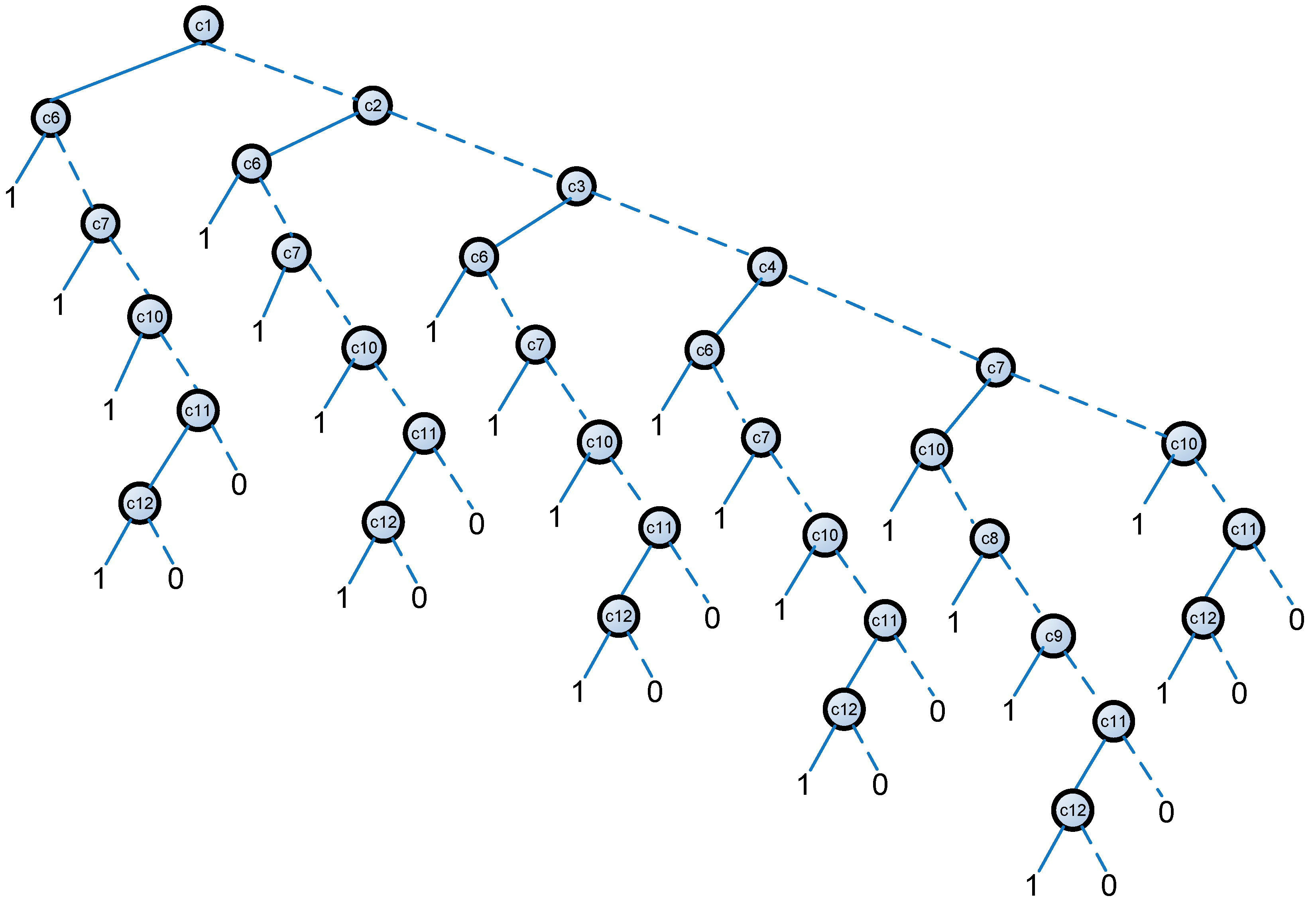
- CS1: q6 q1
- CS2: q7 (1−q6) q1
- CS3: q10 (1−q7) (1−q6) q1
- CS4: q12 q11 (1−q10) (1−q7) (1−q6) q1
- CS5: q6 q2 (1−q1)
- CS6: q7 (1−q6) q2 (1−q1)
- CS7: q10 (1−q7) (1−q6) q2 (1−q1)
- CS8: q12 q11 (1−q10) (1−q7) (1−q6) q2 (1−q1)
- CS9: q6 q3 (1−q2) (1−q1)
- CS10: q7 (1−q6) q3 (1-q2) (1-q1)
- CS11: q10 (1-q7) (1−q6) q3 (1−q2) (1−q1)
- CS12: q12 q11 (1−q10) (1−q7) (1−q6) q3 (1−q2) (1−q1)
- CS13: q6 q4 (1−q3) (1−q2) (1−q1)
- CS14: q7 (1−q6) q4 (1−q3) (1−q2) (1−q1)
- CS15: q10 (1−q7) (1−q6) q4 (1−q3) (1−q2) (1−q1)
- CS16: q12 q11 (1−q10) (1−q7) (1−q6) q4 (1−q3) (1−q2) (1−q1)
- CS17: q10 q7 (1−q4) (1−q3) (1−q2) (1−q1)
- CS18: q8 (1−q10) q7 (1−q4) (1−q3) (1−q2) (1−q1)
- CS19: q9 (1−q8) (1−q10) q7 (1−q4) (1−q3) (1−q2) (1−q1)
- CS20: q12 q011 (1−q9) (1−q8) (1−q10) q7 (1−q4) (1−q3) (1−q2) (1−q1)
- CS21: q10 (1−q7) (1−q4) (1−q3) (1−q2) (1−q1)
- CS22: q12 q11 (1−q10) (1−q7) (1−q4) (1−q3) (1−q2) (1−q1)
3. Dynamic Analysis
- a.
- Constant unreliabilityThe probability of the events or components is constant over the time., where K is a constant valued between 0 and 1.
- b.
- Exponential increasing unreliabilityThe probability function assigned is defined in Equation (1):where is a parameter that takes only positive values and determines how quickly the unreliability increases.
- c.
- Linear decreasing reliabilityThe probability function is defined in Equation (2):where m determines how quickly the unreliability decreases. This model could be acceptable for infant failures of those components that are in the decreasing failure rate of their lifecycle.
- d.
- Periodic unreliabilityThe unreliability of the components has a periodic behavior. The expression used for this assignment is given by Equation (3):with n = 1, 2, 3…, where:
- is a parameter that takes only positive values and determines the velocity of the unreliability rising.
- is a parameter that determines the size of the period
4. Importance Measurement
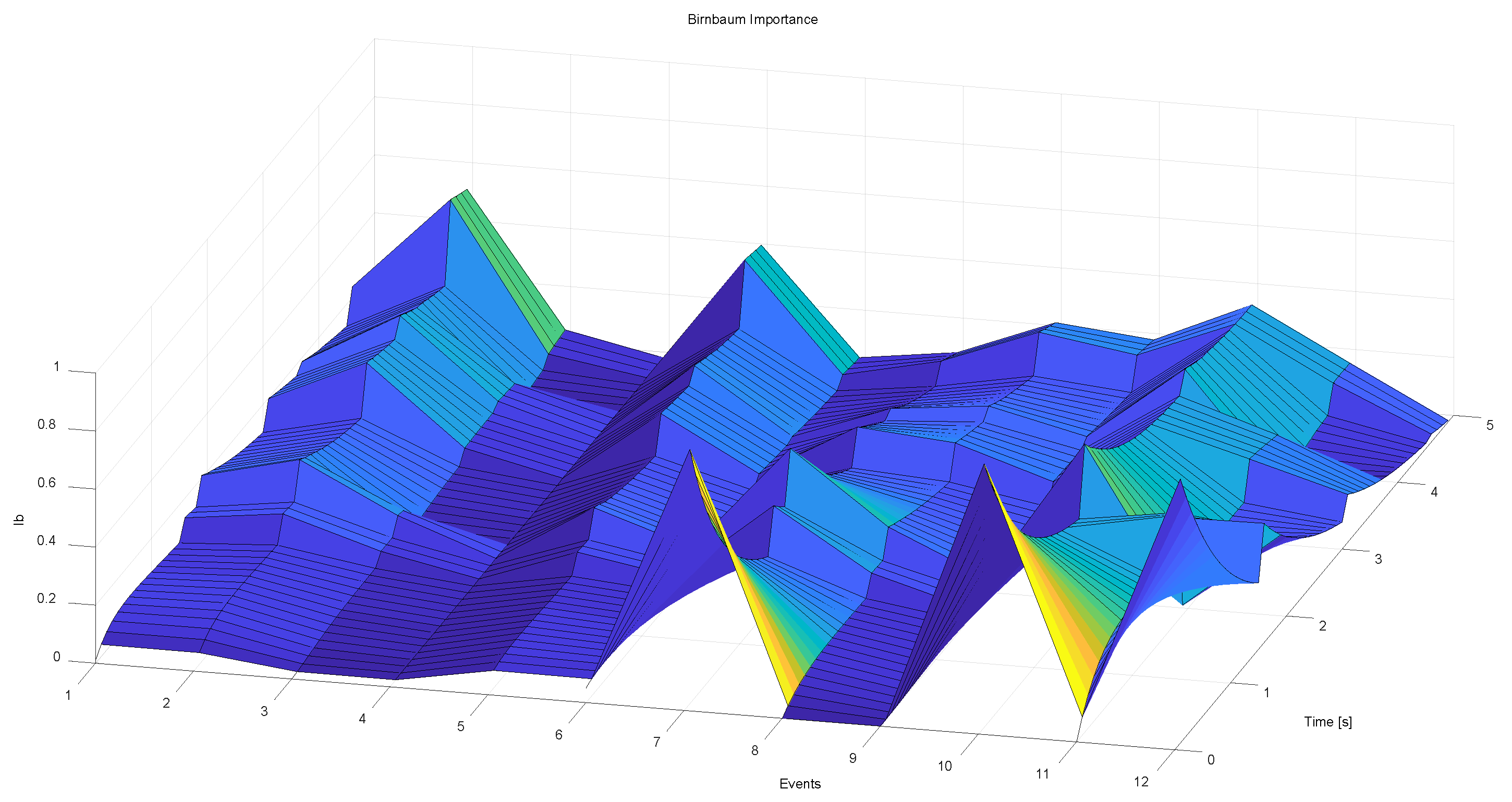
- is the Birnbaum IM value of the kth component;
- is the unreliability of the system;
- , is the probability assigned to the kth component.
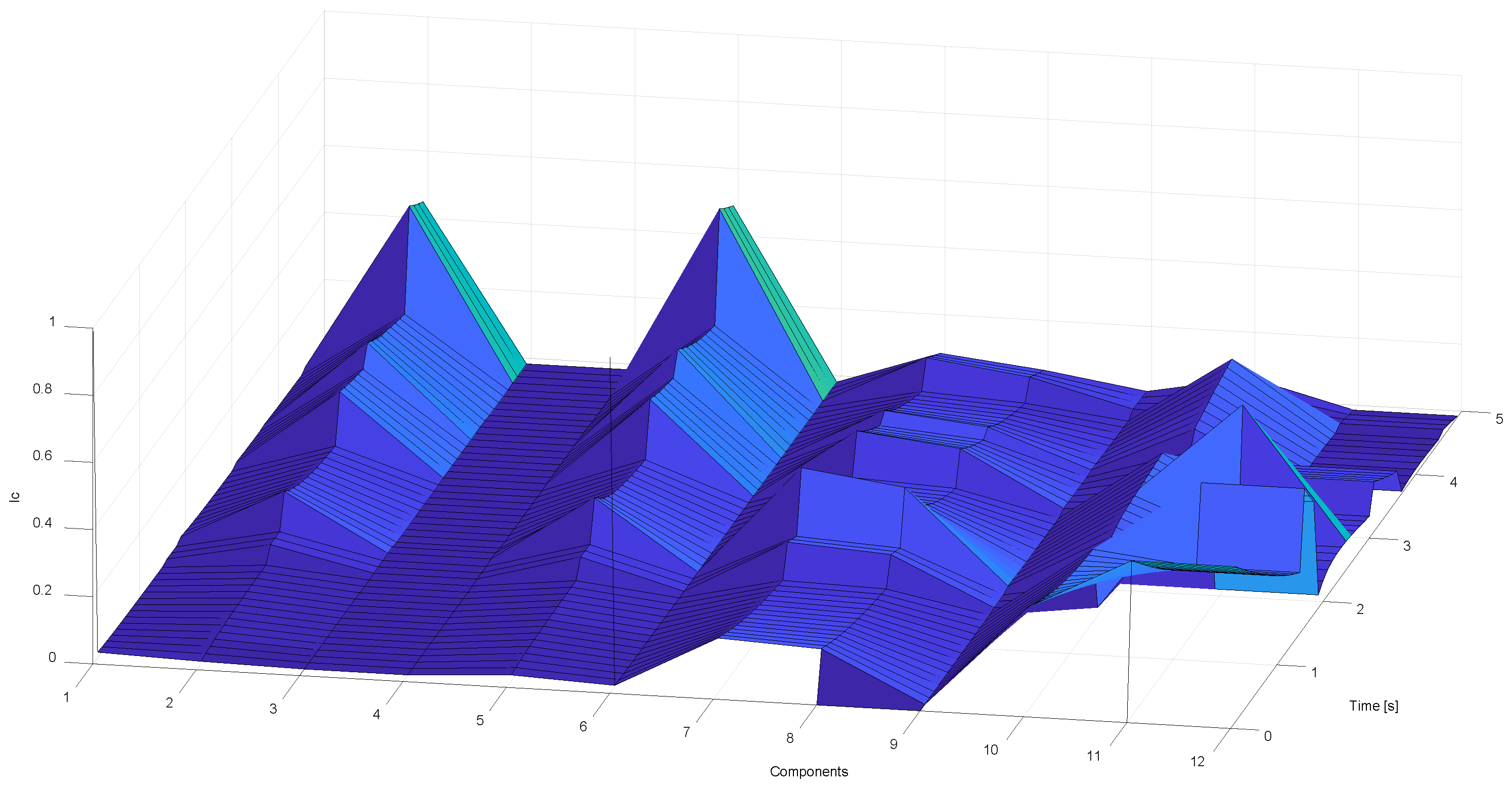
- is the Birnbaum IM of the kth component;
- is the probability assigned to the kth component;
- is the unreliability of the system.
5. Procedure for Maintenance
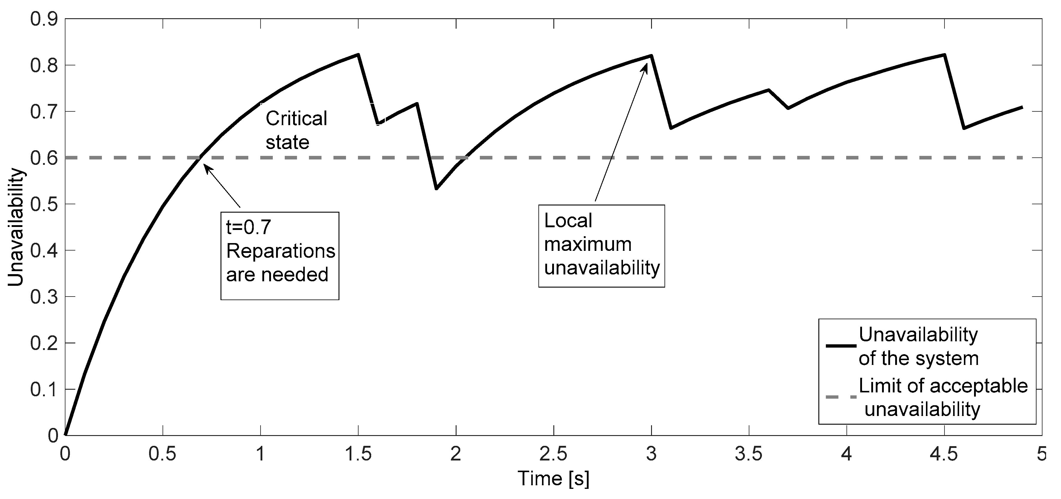
- To determine the reliability of the system and its components at a certain moment;
- To identify critical operating states of the system and its components;
- To determine the optimal time to carry out a preventive task and to choose the components to be repaired or replaced;
- To determine the repairs or replacements necessary to ensure a certain reliability of the system for a period of time.
6. Conclusions
Author Contributions
Funding
Conflicts of Interest
References
- Muñoz, C.Q.G.; Márquez, F.P.G. Future maintenance management in renewable energies. In Renewable Energies; Springer: Berlin/Heidelberg, Germany, 2018; pp. 149–159. [Google Scholar]
- Council, G.W.E. Global Wind Report; GWEC: Brussels, Belgium, 2019. [Google Scholar]
- Qiao, W.; Lu, D. A survey on wind turbine condition monitoring and fault diagnosis—part i: Components and subsystems. IEEE Trans. Ind. Electron. 2015, 62, 6536–6545. [Google Scholar] [CrossRef]
- Marquez, F.G. An approach to remote condition monitoring systems management. In Proceedings of the 2006 IET International Conference On Railway Condition Monitoring, Birmingham, UK, 29–30 November 2006. [Google Scholar]
- Márquez, F.P.G.; Pedregal, D.J. Applied RCM2 algorithms based on statistical methods. Int. J. Autom. Comput. 2007, 4, 109–116. [Google Scholar] [CrossRef]
- Njiri, J.G.; Soeffker, D. State-of-the-art in wind turbine control: Trends and challenges. Renew. Sustain. Energy Rev. 2016, 60, 377–393. [Google Scholar] [CrossRef]
- Spiess, H.; Lobsiger-Kägi, E.; Carabias-Hütter, V.; Marcolla, A. Future acceptance of wind energy production: Exploring future local acceptance of wind energy production in a swiss alpine region. Technol. Forecast. Soc. Chang. 2015, 101, 263–274. [Google Scholar] [CrossRef]
- Petković, D.; Pavlović, N.T.; Ćojbašić, Ž. Wind farm efficiency by adaptive neuro-fuzzy strategy. Int. J. Electr. Power Energy Syst. 2016, 81, 215–221. [Google Scholar] [CrossRef]
- Márquez, F.P.G.; Lev, B. Advanced Business Analytics; Springer: Berlin/Heidelberg, Germany, 2015. [Google Scholar]
- Sarker, B.R.; Faiz, T.I. Minimizing maintenance cost for offshore wind turbines following multi-level opportunistic preventive strategy. Renew. Energy 2016, 85, 104–113. [Google Scholar] [CrossRef]
- Pliego Marugán, A.; García Márquez, F.P. Advanced analytics for detection and diagnosis of false alarms and faults: A real case study. Wind Energy 2019, 22, 1622–1635. [Google Scholar] [CrossRef]
- Márquez, F.P.G.; Pardo, I.P.G.; Nieto, M.R.M. Competitiveness based on logistic management: A real case study. Ann. Oper. Res. 2015, 233, 157–169. [Google Scholar]
- Shafiee, M.; Sørensen, J.D. Maintenance optimization and inspection planning of wind energy assets: Models, methods and strategies. Reliab. Eng. Syst. Saf. 2019, 192, 105993. [Google Scholar] [CrossRef]
- Tavner, P.; Gindele, R.; Faulstich, S.; Hahn, B.; Whittle, M.; Greenwood, D. Study of Effects of Weather & Location on Wind Turbine Failure Rates. In Proceedings of the European Wind Energy Conference EWEC, Warsaw, Poland, 15 March 2010. [Google Scholar]
- Marquez, F.G.; Singh, V.; Papaelias, M. A Review of Wind Turbine Maintenance Management Procedures. In Proceedings of the Eighth International Conference on Condition Monitoring and Machinery Failure Prevention Technologies, Cardiff, UK, 20–22 June 2011; pp. 1–14. [Google Scholar]
- Márquez, F.P.G.; Karyotakis, A.; Papaelias, M. Renewable Energies: Business Outlook 2050; Springer: Berlin/Heidelberg, Germany, 2018. [Google Scholar]
- Pérez, J.M.P.; Márquez, F.P.G.; Hernández, D.R. Economic viability analysis for icing blades detection in wind turbines. J. Clean. Prod. 2016, 135, 1150–1160. [Google Scholar] [CrossRef]
- Bangalore, P.; Patriksson, M. Analysis of scada data for early fault detection, with application to the maintenance management of wind turbines. Renew. Energy 2018, 115, 521–532. [Google Scholar] [CrossRef]
- Marugán, A.P.; Márquez, F.P.G.; Papaelias, M. Multivariable Analysis for Advanced Analytics of Wind Turbine Management. In Proceedings of the Tenth International Conference on Management Science and Engineering Management, Baku, Azerbaijan, 30 August–2 September 2016; pp. 319–328. [Google Scholar]
- Márquez, F.P.G. A new method for maintenance management employing principal component analysis. Struct. Durab. Health Monit. 2010, 6, 89–99. [Google Scholar]
- Pedregal, D.J.; García, F.P.; Roberts, C. An algorithmic approach for maintenance management based on advanced state space systems and harmonic regressions. Ann. Oper. Res. 2009, 166, 109–124. [Google Scholar] [CrossRef]
- Marugán, A.P.; Chacón, A.M.P.; Márquez, F.P.G. Reliability analysis of detecting false alarms that employ neural networks: A real case study on wind turbines. Reliab. Eng. Syst. Saf. 2019, 191, 106574. [Google Scholar] [CrossRef]
- Schlechtingen, M.; Santos, I.F. Comparative analysis of neural network and regression based condition monitoring approaches for wind turbine fault detection. Mech. Syst. Signal Process. 2011, 25, 1849–1875. [Google Scholar] [CrossRef]
- Gómez Muñoz, C.Q.; García Marquez, F.P.; Hernandez Crespo, B.; Makaya, K. Structural health monitoring for delamination detection and location in wind turbine blades employing guided waves. Wind Energy 2019, 22, 698–711. [Google Scholar] [CrossRef]
- Arcos Jiménez, A.; Gómez Muñoz, C.Q.; García Márquez, F.P. Machine learning for wind turbine blades maintenance management. Energies 2018, 11, 13. [Google Scholar] [CrossRef]
- Gómez, C.; García, F.; Arcos, A.; Cheng, L.; Kogia, M.; Mohimi, A.; Papaelias, M. A heuristic method for detecting and locating faults employing electromagnetic acoustic transducers. Eksploat. Niezawodn. 2017, 19. [Google Scholar] [CrossRef]
- Gómez, C.Q.; Villegas, M.A.; García, F.P.; Pedregal, D.J. Big data and web intelligence for condition monitoring: A case study on wind turbines. In Big Data: Concepts, Methodologies, Tools, and Applications; IGI Global: Hershey, PA, USA, 2016; pp. 1295–1308. [Google Scholar]
- Ramirez, I.S.; Muñoz, C.Q.G.; Marquez, F.P.G. A condition monitoring system for blades of wind turbine maintenance management. In Proceedings of the Tenth International Conference on Management Science and Engineering Management, Baku, Azerbaijan, 30 August–2 September 2016; pp. 3–11. [Google Scholar]
- Roshanmanesh, S.; Hayati, F.; Kappatos, V.; Marquez, F.P.G.; Marugán, A.P.; Muñoz, C.Q.G.; Selcuk, C.; Gan, T.-H.; Papaelias, M. Drive-Train Condition Monitoring for Offshore Wind and Tidal Turbines, 2nd ed. In Proceedings of the International Conference on Renewable Energies Offshore (Renew 2016), Lisbon, Portugal, 24–26 October 2016. [Google Scholar]
- Jiménez, A.A.; Márquez, F.P.G.; Moraleda, V.B.; Muñoz, C.Q.G. Linear and nonlinear features and machine learning for wind turbine blade ice detection and diagnosis. Renew. Energy 2019, 132, 1034–1048. [Google Scholar] [CrossRef]
- García Márquez, F.P.; Segovia Ramírez, I.; Pliego Marugán, A. Decision making using logical decision tree and binary decision diagrams: A real case study of wind turbine manufacturing. Energies 2019, 12, 1753. [Google Scholar] [CrossRef]
- Pliego Marugán, A.; García Márquez, F.P.; Lev, B. Optimal decision-making via binary decision diagrams for investments under a risky environment. Int. J. Prod. Res. 2017, 55, 5271–5286. [Google Scholar] [CrossRef]
- Kempener, R.; Assoumou, E.; Chiodi, A.; Ciorba, U.; Gaeta, M.; Gielen, D.; Hamasaki, H.; Kanudia, A.; Kober, T.; Labriet, M. A global renewable energy roadmap: Comparing energy systems models with irena’s remap 2030 project. In Informing Energy and Climate Policies Using Energy Systems Models; Springer: Berlin/Heidelberg, Germany, 2015; pp. 43–67. [Google Scholar]
- Muñoz, C.Q.G.; Márquez, F.P.G.; Tomás, J.M.S. Ice detection using thermal infrared radiometry on wind turbine blades. Measurement 2016, 93, 157–163. [Google Scholar] [CrossRef]
- Jiménez, A.A.; Zhang, L.; Muñoz, C.Q.G.; Márquez, F.P.G. Maintenance management based on machine learning and nonlinear features in wind turbines. Renew. Energy 2020, 146, 316–328. [Google Scholar] [CrossRef]
- García Márquez, F.P.; García-Pardo, I.P. Principal component analysis applied to filtered signals for maintenance management. Qual. Reliab. Eng. Int. 2010, 26, 523–527. [Google Scholar] [CrossRef]
- Garcia Marquez, F.P.; Pliego Marugan, A.; Pérez, P.; María, J.; Hillmansen, S.; Papaelias, M. Optimal dynamic analysis of electrical/electronic components in wind turbines. Energies 2017, 10, 1111. [Google Scholar] [CrossRef]
- Pliego Marugán, A.; Garcia Márquez, F.P. Fault-tree dynamic analysis. In Proceedings of the Eleventh International Conference on Condition Monitoring and Machinery Failure Prevention Technologies CM, Manchester, UK, 10–12 June 2014; pp. 10–12. [Google Scholar]
- Márquez, F.P.G.; Pérez, J.M.P.; Marugán, A.P.; Papaelias, M. Identification of critical components of wind turbines using fta over the time. Renew. Energy 2016, 87, 869–883. [Google Scholar] [CrossRef]
- Márquez, F.G.; Papaelias, J.; Hermosa, R.R. Wind turbines maintenance management based on fta and bdd. In Proceedings of the International Conference on Renewable Energies and Power Quality (ICREPQ’12), Santiago de Compostela, Spain, 28–30 March 2012; pp. 4–6. [Google Scholar]
- Lee, J.; Ye, Y.-H.; Huang, X.; Yang, R.-L. Binary-decision-diagram-based decomposition of boolean functions into reversible logic elements. Theor. Comput. Sci. 2020, 814, 120–134. [Google Scholar] [CrossRef]
- Jiménez, A.A.; Muñoz, C.Q.G.; Márquez, F.P.G. Dirt and mud detection and diagnosis on a wind turbine blade employing guided waves and supervised learning classifiers. Reliab. Eng. Syst. Saf. 2019, 184, 2–12. [Google Scholar] [CrossRef]
- Muñoz, C.Q.G.; Marquez, F.P.G.; Lev, B.; Arcos, A. New pipe notch detection and location method for short distances employing ultrasonic guided waves. Acta Acust. United Acust. 2017, 103, 772–781. [Google Scholar] [CrossRef]
- Pedro, F.; Marquez, G. Binary decision diagrams applied to fault tree analysis. In Proceedings of the 4th IET International Conference on Railway Condition Monitoring (RCM 2008), Birmingham, UK, 18–20 June 2008. [Google Scholar]
- Li, Z.; Wang, Z.; Ren, Y.; Yang, D.; Lv, X. A novel reliability estimation method of multi-state system based on structure learning algorithm nowatorska metoda oceny niezawodności systemów wielostanowych w oparciu o algorytm uczenia struktury. Eksploatacja I Niezawodnosc 2020, 22, 170. [Google Scholar] [CrossRef]
- Wang, H.; Duan, F.; Ma, J. Reliability analysis of complex uncertainty multi-state system based on bayesian network zastosowanie sieci bayesowskiej do analizy niezawodności złożonych systemów wielostanowych w warunkach niepewności. Eksploatacja I Niezawodnosc 2019, 21, 419. [Google Scholar] [CrossRef]
- Bucci, P.; Kirschenbaum, J.; Mangan, L.A.; Aldemir, T.; Smith, C.; Wood, T. Construction of event-tree/fault-tree models from a markov approach to dynamic system reliability. Reliab. Eng. Syst. Saf. 2008, 93, 1616–1627. [Google Scholar] [CrossRef]
- Bhagavatula, A.; Tao, J.; Dunnett, S.; Bell, P. A New Methodology for Automatic Fault Tree Construction Based on Component and Mark Libraries; Safety and Reliability; Taylor & Francis: Abingdon, UK, 2016; pp. 62–76. [Google Scholar]
- Majdara, A.; Wakabayashi, T. Component-based modeling of systems for automated fault tree generation. Reliab. Eng. Syst. Saf. 2009, 94, 1076–1086. [Google Scholar] [CrossRef]
- Liu, X.; Wang, Z.; Ren, Y.; Liu, L. Modeling method of sysml-based reliability block diagram. In Proceedings of the 2013 International Conference on Mechatronic Sciences, Electric Engineering and Computer (MEC), Shenyang, China, 20–22 December 2013; pp. 206–209. [Google Scholar]
- Li, K.; Yi, R.; Ma, Z. Reliability analysis of dynamic reliability blocks through conversion into dynamic bayesian networks. In Proceedings of the 2016 IEEE International Conference on Industrial Engineering and Engineering Management (IEEM), Bali, Indonesia, 5–7 December 2016; pp. 1330–1334. [Google Scholar]
- Mi, J.; Li, Y.; Huang, H.-Z.; Liu, Y.; Zhang, X. Reliability analysis of multi-state systems with common cause failure based on bayesian networks. In Proceedings of the 2012 International Conference on Quality, Reliability, Risk, Maintenance, and Safety Engineering, Chengdu, China, 15–18 June 2012; pp. 1117–1121. [Google Scholar]
- Montani, S.; Portinale, L.; Bobbio, A.; Codetta-Raiteri, D. Radyban: A tool for reliability analysis of dynamic fault trees through conversion into dynamic bayesian networks. Reliab. Eng. Syst. Saf. 2008, 93, 922–932. [Google Scholar] [CrossRef]
- Rauzy, A. Mathematical foundations of minimal cutsets. IEEE Trans. Reliab. 2001, 50, 389–396. [Google Scholar] [CrossRef]
- Dutuit, Y.; Rauzy, A. Efficient algorithms to assess component and gate importance in fault tree analysis. Reliab. Eng. Syst. Saf. 2001, 72, 213–222. [Google Scholar] [CrossRef]
- Marugan, A.P.; Márquez, F.P.G. Decision-Making Management: A Tutorial and Applications; Academic Press: Cambridge, MA, USA, 2017. [Google Scholar]
- Hansen, A.D.; Michalke, G. Fault ride-through capability of dfig wind turbines. Renew. Energy 2007, 32, 1594–1610. [Google Scholar] [CrossRef]
- Lu, B.; Li, Y.; Wu, X.; Yang, Z. A review of recent advances in wt condition monitoring and fault diagnosis. In Proceedings of the Power Electronics and Machines in Wind Applications, Lincoln, NE, USA, 24–26 June 2009; pp. 24–26. [Google Scholar]
- Popa, L.M.; Jensen, B.-B.; Ritchie, E.; Boldea, I. Condition monitoring of wind generators. In Proceedings of the 38th IAS Annual Meeting on Conference Record of the Industry Applications Conference, Salt Lake City, UT, USA, 12–16 October 2003; pp. 1839–1846. [Google Scholar]
- Wu, A.P.; Chapman, P.L. Simple expressions for optimal current waveforms for permanent-magnet synchronous machine drives. IEEE Trans. Energy Convers. 2005, 20, 151–157. [Google Scholar] [CrossRef]
- Lee, C.-Y. Representation of switching circuits by binary-decision programs. Bell Syst. Tech. J. 1959, 38, 985–999. [Google Scholar] [CrossRef]
- Moret, B.M. Decision trees and diagrams. ACM Comput. Surv. (CSUR) 1982, 14, 593–623. [Google Scholar] [CrossRef]
- Akers, S.B. Binary decision diagrams. IEEE Trans. Comput. 1978, C-27, 509–516. [Google Scholar] [CrossRef]
- Bryant, R.E. Graph-based algorithms for boolean function manipulation. Comput. IEEE Trans. 1986, 100, 677–691. [Google Scholar] [CrossRef]
- Fujita, M.; Fujisawa, H.; Kawato, N. Evaluation and Improvement of Boolean Comparison Method Based on Binary Decision Diagrams; ICCAD, Citeseer: Santa Clara, CA, USA, 1988; pp. 2–5. [Google Scholar]
- Pliego Marugán, A.; García Márquez, F.P.; Lorente, J. Decision making process via binary decision diagram. Int. J. Manag. Sci. Eng. Manag. 2015, 10, 3–8. [Google Scholar] [CrossRef]
- Bartlett, L.M. Progression of the binary decision diagram conversion methods. In In Proceedings of the 21st International SystemsSafety Conference, Ottowa, ON, Canada, 2–4 August 2003. [Google Scholar]
- Cormen, T.H.; Leiserson, C.E.; Rivest, R.L.; Stein, C. Elementary graph algorithms. Introd. Algorithms 2009, 1, 540–549. [Google Scholar]
- Jensen, R.M.; Veloso, M.M. Obdd-based universal planning for synchronized agents in non-deterministic domains. J. Artif. Intell. Res. 2000, 13, 189–226. [Google Scholar] [CrossRef]
- Malik, S.; Wang, A.R.; Brayton, R.K.; Sangiovanni-Vincentelli, A. Logic verification using binary decision diagrams in a logic synthesis environment. In Proceedings of the IEEE International Conference on Computer-Aided Design (ICCAD-89) Digest of Technical Papers, Santa Clara, CA, USA, 7–10 November 1988; pp. 6–9. [Google Scholar]
- Xie, M.; Tan, K.; Goh, K.; Huang, X. Optimum prioritisation and resource allocation based on fault tree analysis. Int. J. Qual. Reliab. Manag. 2000, 17, 189–199. [Google Scholar] [CrossRef]
- Coudert, O.; Madre, J.C. Metaprime: An interactive fault-tree analyzer. IEEE Trans. Reliab. 1994, 43, 121–127. [Google Scholar] [CrossRef]
- Reay, K.A.; Andrews, J.D. A fault tree analysis strategy using binary decision diagrams. Reliab. Eng. Syst. Saf. 2002, 78, 45–56. [Google Scholar] [CrossRef]
- Jung, W.S.; Han, S.H.; Ha, J. A fast bdd algorithm for large coherent fault trees analysis. Reliab. Eng. Syst. Saf. 2004, 83, 369–374. [Google Scholar] [CrossRef]
- Borgonovo, E. Differential, criticality and birnbaum importance measures: An application to basic event, groups and sscs in event trees and binary decision diagrams. Reliab. Eng. Syst. Saf. 2007, 92, 1458–1467. [Google Scholar] [CrossRef]
- Cheok, M.C.; Parry, G.W.; Sherry, R.R. Use of importance measures in risk-informed regulatory applications. Reliab. Eng. Syst. Saf. 1998, 60, 213–226. [Google Scholar] [CrossRef]
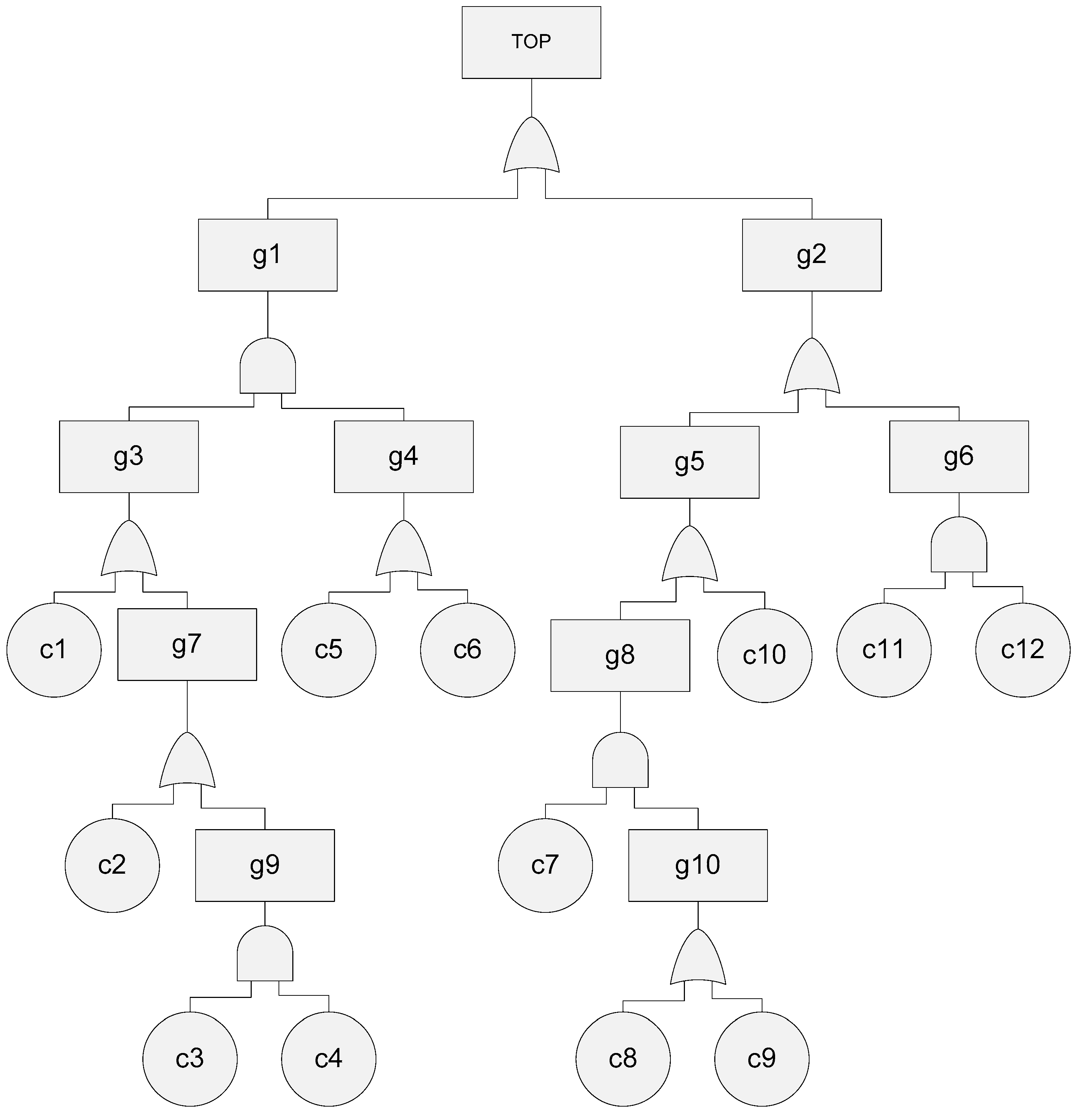
| Critical Generator Failure | g1 | Abnormal Vibration G | c1 |
| Power electronics (PE) and electric controls failure | g2 | Cracks | c2 |
| Mechanical failure (generator) | g3 | Imbalance | c3 |
| Electrical failure (generator) | g4 | Asymmetry | c4 |
| Electrical fault (PE) | g5 | Short circuit (generator) | c5 |
| Mechanical fault (PE) | g6 | Open circuit (generator) | c6 |
| Bearing generator fault | g7 | Gate drive circuit | c7 |
| Electrical failure | g8 | Short circuit (electronics) | c8 |
| Abnormal signals A | g9 | Open circuit (electronics) | c9 |
| Power electronic | g10 | Broken bars | c10 |
| Corrosion | c11 | ||
| Terminals damage | c12 |
| Ranking Method | TLDR | DFS | BFS | Level | AND |
|---|---|---|---|---|---|
| Number of CSs | 38 | 22 | 23 | 26 | 23 |
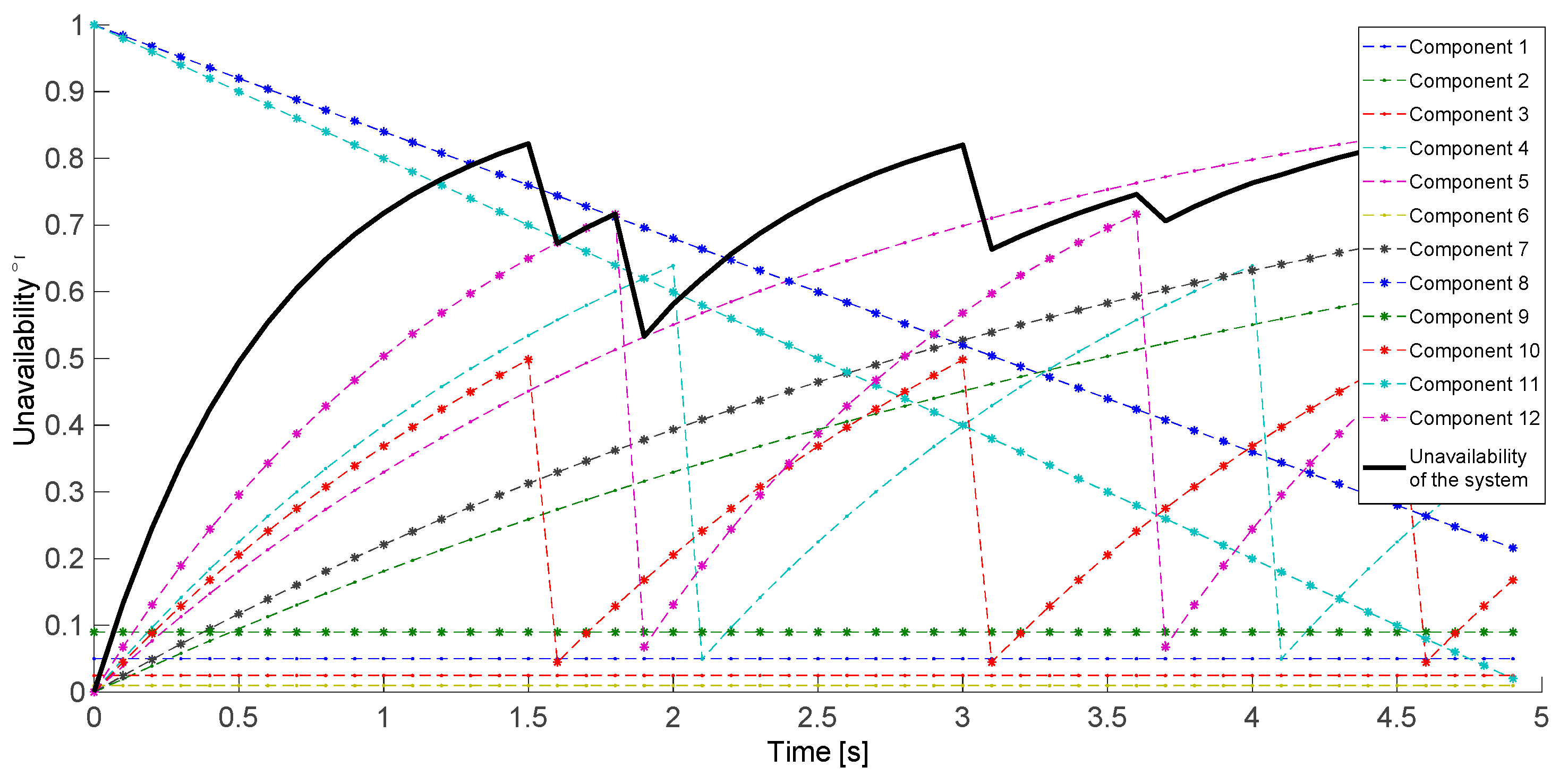
| Components | Probability Model | Parameters |
|---|---|---|
| Component 1 | Constant | K = 0.5 |
| Component 2 | Exponential increasing | λ = 0.2 |
| Component 3 | Constant | K = 0.025 |
| Component 4 | Periodic | λ = 0.51, = 2 |
| Component 5 | Exponential increasing | λ = 0.4 |
| Component 6 | Constant | K = 0.01 |
| Component 7 | Exponential increasing | λ = 0.25 |
| Component 8 | Linear decreasing | m = 0.16 |
| Component 9 | Constant | K = 0.09 |
| Component 10 | Periodic | λ = 0.46, = 1.5 |
| Component 11 | Linear decreasing | m = 0.16 |
| Component 12 | Periodic | λ = 0.7, = 0.8 |
© 2020 by the authors. Licensee MDPI, Basel, Switzerland. This article is an open access article distributed under the terms and conditions of the Creative Commons Attribution (CC BY) license (http://creativecommons.org/licenses/by/4.0/).
Share and Cite
García Márquez, F.P.; Segovia Ramírez, I.; Mohammadi-Ivatloo, B.; Marugán, A.P. Reliability Dynamic Analysis by Fault Trees and Binary Decision Diagrams. Information 2020, 11, 324. https://doi.org/10.3390/info11060324
García Márquez FP, Segovia Ramírez I, Mohammadi-Ivatloo B, Marugán AP. Reliability Dynamic Analysis by Fault Trees and Binary Decision Diagrams. Information. 2020; 11(6):324. https://doi.org/10.3390/info11060324
Chicago/Turabian StyleGarcía Márquez, Fausto Pedro, Isaac Segovia Ramírez, Behnam Mohammadi-Ivatloo, and Alberto Pliego Marugán. 2020. "Reliability Dynamic Analysis by Fault Trees and Binary Decision Diagrams" Information 11, no. 6: 324. https://doi.org/10.3390/info11060324
APA StyleGarcía Márquez, F. P., Segovia Ramírez, I., Mohammadi-Ivatloo, B., & Marugán, A. P. (2020). Reliability Dynamic Analysis by Fault Trees and Binary Decision Diagrams. Information, 11(6), 324. https://doi.org/10.3390/info11060324


