Article

GAP: Geometric Aggregation of Popularity Metrics

Information Technologies Institute, Centre of Research and Technology Hellas, 6th km Harilaou-Thermi, 57001 Thessaloniki, Greece
*
Author to whom correspondence should be addressed.
Information 2020, 11(6), 323; https://doi.org/10.3390/info11060323
Submission received: 13 May 2020 / Revised: 8 June 2020 / Accepted: 11 June 2020 / Published: 15 June 2020

Abstract

:
Estimating and analyzing the popularity of an entity is an important task for professionals in several areas, e.g., music, social media, and cinema. Furthermore, the ample availability of online data should enhance our insights into the collective consumer behavior. However, effectively modeling popularity and integrating diverse data sources are very challenging problems with no consensus on the optimal approach to tackle them. To this end, we propose a non-linear method for popularity metric aggregation based on geometrical shapes derived from the individual metrics’ values, termed Geometric Aggregation of Popularity metrics (GAP). In this work, we particularly focus on the estimation of artist popularity by aggregating web-based artist popularity metrics. Finally, even though the most natural choice for metric aggregation would be a linear model, our approach leads to stronger rank correlation and non-linear correlation scores compared to linear aggregation schemes. More precisely, our approach outperforms the simple average method in five out of seven evaluation measures.

1. Introduction

Popularity is without a doubt an abstract notion that is used to express how much attention a certain item, person, or concept has received lately. Today, the estimation of an entity’s popularity is desirable in many areas such as music [1], social media [2], science [3], cinema [4], and the Internet [5]. The temporal dynamical patterns of popularity gain vary from entity to entity and can exhibit either viral or steady behavior [6]. Additionally, when multiple metrics concerning performance in general are available for each entity, an optimal approach for the aggregation of the metrics or the rankings is certainly of interest [7,8]. Many such methods have been proposed in the multi-criteria decision analysis (MCDA) research literature [9,10].
This study particularly focuses on the estimation of music artist popularity. For music related products, the traditional way to measure their popularity has been through sales and music top charts. Currently, there is an abundance of online sources that we can draw data from, including streams, downloads, and queries related to music tracks, albums, artists, and musical genres. The consideration of these modern sources as popularity metrics is reasonable for a number of reasons. The music consumer interest is directed to online music sources rather than the traditional record stores and the purchasing of physical albums. Furthermore, not all countries release charts, or if they do, they may not be easy to obtain, so the comparability among countries is hard with the traditional methods of popularity determination. Therefore, we consider web-based artist popularity metrics, such as YouTube views, Spotify popularity, and Facebook mentions, for aggregation.
Determining the popularity of a music track, artist, or genre has attracted increased research interest during the last few years. Many ways to define music popularity have been proposed making use of the online available information from posts on microblog websites [11,12,13,14] and in the blogosphere [15], search queries and the number of shared files in peer-to-peer networks [13,16], play counts in social media music sites such as Last.fm [12,17], the amount of time of radio play, the music industry awards that it received [18], and popularity indices provided by streaming platforms such as Spotify [17]. Of course, the traditional ways of determining music popularity such as the Billboard Magazine chart are also used for comparison with the modern web-based popularity indices [16,19]. In [18], the authors claimed that three factors, the music acoustic content, the artist’s reputation, and the number of comments regarding the track, in synergy are able to classify a music track as popular or not, with high accuracy. Furthermore, the level of public recognition of a music track has been investigated providing a different aspect in the evaluation of music entities [20].
Although many studies have been conducted on the estimation of artist popularity, the determination of an evaluation method for such popularity scores remains a challenge as no general agreement regarding an acceptable ground truth has been established. This leads researchers to evaluation through comparison with several other existing popularity metrics such as Spotify popularity, page counts, and the charts. In Table 1, we present the evaluation methods (and ground truth) followed by research papers for their proposed popularity scores.
Moreover, according to our knowledge, all popularity scores that have been proposed in the research literature until today are univariate, while the method that we propose herein is the first to combine several diverse sources and metrics of popularity in order to summarize the whole picture of an entity’s popularity. Although the most natural choice for metric aggregation is a simple average, the handling of many different sources is clearly not obvious and might be useful to evaluate and compare other non-linear methods as well. Furthermore, being popular with regard to one or some of the monitored metrics is sufficient to characterize an entity as popular; hence, the robustness against such cases is desirable when using a metric aggregation method. Our method leverages the area of geometrical shapes formed by the metrics’ values in a non-linear manner; thus, we name it Geometric Aggregation of Popularity metrics (GAP0 and GAP1 are two variations of the same concept). Finally, we conduct a comparative study including the average normalized metric value and two other non-linear metric aggregation methods.
The rest of the paper is structured as follows. In Section 2, the proposed methodology is illustrated. In Section 3, the experimental setup is elaborated and results are presented, and in Section 4, conclusions are given.

2. Geometric Aggregation of Popularity Metrics

2.1. Definition

Here, we propose an aggregation method that leverages multi-source web-based information in order to assess the level of an entity’s current popularity. In order to determine the popularity of entity e at time t, we first normalize the respective metric values v e , t , i for i = 1 , , n (where n is the number of monitored metrics for the entity under study) to [0, 1] using a power transformation as in Equation (1):
m e , i , t = v e , t , i P T
where T is the chosen maximum power transformed value, cf. below, v e , t , i is the initial value of metric i at time t for entity e, P = l o g ( T ) l o g ( V t , i ) = l o g V t , i ( T ) with V t , i the maximum of v e , t , i over all entities e, and m e , i , t the normalized metric value. The choice of the exponent P derives from the observation that V t , i P = T and 0 P = 0 , which result in m e , i , t [ 0 , 1 ] , given that v e , t , i [ 0 , V t , i ] . We did not opt for a simple “divide by maximum” or “min-max” normalization because there are metrics with huge variation such as YouTube views that in some cases reach billions, and thus, artists with millions of views would seem non-important. Furthermore, we did not opt for a log transform because there are metrics with a small range such as Spotify popularity, with values from zero to 100. In this case, after the transformation, all normalized values would be between zero and ∼4.61, and a significant Spotify popularity increase, e.g., from 50 to 80 (being 3.91 and 4.38 after log transformation), would not affect the aggregated popularity correspondingly. Power transform alleviates both issues with a relatively high T = 100, which could be optimized if one considers an appropriate ground truth.
After the normalization, we considered the unit circle and n equidistant points k i on it. On each radius from k i to the center, we selected the point l i with distance m e , i , t from k i . Geometric Aggregation of Popularity metrics (GAP0) is then defined as:
E o u t E i n E o u t · 100
where E o u t is the area of the outer regular n-sided polygon determined by k i and E i n is the area of the inner polygon determined by l i . If an artist performs best on all metrics, the inner polygon would coincide with the circle’s center, and the geometric aggregation of popularity metrics would be 100; while if an artist performs worst on all metrics, the inner polygon would coincide with the outer regular polygon, and the geometric aggregation of popularity metrics would be zero. All other cases result in intermediate values. Of course, different orders of the metrics result in different popularity scores; thus for consistency, we first sorted the metric values and then applied the computations on the sorted sequence of metrics.
In Figure 1a, an example case for the computation of Geometric Aggregation of Popularity metrics (GAP0) is exemplified concerning the artist “The Rasmus” on 2 April 2019, resulting in GAP0 = 62.0. A second approach on Geometric Aggregation of Popularity metrics (GAP1) was to represent the metrics by the sides of the polygon and not by the vertexes. Thus, the inner polygon in this case was the aggregate of n isosceles triangles with side length equal to 1 m e , i , t , as depicted in Figure 1b. The popularity was then calculated as in the first approach by applying Equation (2), resulting in GAP1 = 60.4. Furthermore, the simple average of the normalized metrics multiplied by 100 was 38.9.

2.2. Additional Analytical Results on Geometric Aggregation of Popularity Metrics

The calculation of GAP0(m) and GAP1(m), while not straightforward, is actually very simple given the vector of normalized metric values m = { m e , i , t | i = 1 , , n } , for entity e at time t:
G A P 0 ( m ) = 1 n i = 1 n m e , i , t + m e , i + 1 , t · ( 1 m e , i , t )
G A P 1 ( m ) = 1 n i = 1 n 2 · m e , i , t m e , i , t 2
where m e , n + 1 , t = m e , 1 , t .
Proof. 
For GAP0(m), the inner polygon’s area is the sum of n triangles’ areas:
i = 1 n 1 2 ( 1 m e , i , t ) · ( 1 m e , i + 1 , t ) · sin θ
where θ = 2 π / n .
The outer polygon’s area is the sum of n equal triangles’ areas: n · ( 1 2 · 1 · 1 · sin θ ) = n · sin θ 2 . Hence, according to Equation (2):
G A P 0 ( m ) = n · sin θ 2 i = 1 n 1 2 ( 1 m e , i , t ) · ( 1 m e , i + 1 , t ) · sin θ n · sin θ 2 = 1 1 n ( 1 m e , i , t ) · ( 1 m e , i + 1 , t ) = 1 ( 1 m e , i , t ) · ( 1 m e , i + 1 , t ) n = 1 n i = 1 n m e , i , t + m e , i + 1 , t ( 1 m e , i , t )
For GAP1(m), the inner polygon’s area is the sum of n isosceles triangles’ areas:
i = 1 n 1 2 ( 1 m e , i , t ) 2 · sin θ
The outer polygon’s area is the same as before:
n · sin θ 2
Hence,
G A P 1 ( m ) = n · sin θ 2 1 2 ( 1 m e , i , t ) 2 · sin θ n · sin θ 2 = 1 1 n ( 1 m e , i , t ) 2 = 1 n i = 1 n 2 · m e , i , t m e , i , t 2
 □
Furthermore, considering the most natural choice for popularity aggregation, i.e., the average normalized metric values (Average Artist Popularity (AAP)):
A A P ( m ) = 1 n i = 1 n m e , i , t
it is remarkable that:
A A P ( m ) G A P 1 ( m ) G A P 0 ( m )
for all sorted m, with m e , i , t [0, 1].
Proof. 
The first part of the inequality is pretty straightforward:
m e , i , t 1 m e , i , t 2 m e , i , t 0 m e , i , t m e , i , t 2 m e , i , t 2 · m e , i , t m e , i , t 2
1 n i = 1 n m e , i , t 1 n i = 1 n 2 · m e , i , t m e , i , t 2 A A P ( m ) G A P 1 ( m )
For the second part of the inequality, we begin with the assumption that m is sorted:
m e , i , t m e , i + 1 , t i = 1 , , n 1
The difference D i between the methods GAP1 and GAP0 per metric i is:
D i = 2 · m e , i , t m e , i , t 2 m e , i , t + m e , i + 1 , t · ( 1 m e , i , t ) = m e , i , t m e , i , t 2 m e , i + 1 , t + m e , i + 1 , t · m e , i , t = m e , i , t ( 1 m e , i , t ) m e , i + 1 , t ( 1 m e , i , t ) = ( 1 m e , i , t ) ( m e , i , t m e , i + 1 , t ) 0 , i = 1 , , n 1
and the corresponding difference for i = n is D n = ( 1 m e , n , t ) ( m e , n , t m e , 1 , t ) ≥ 0. The total difference between the two models then is:
G A P 1 ( m ) G A P 0 ( m ) = 1 n i = 1 n 2 · m e , i , t m e , i , t 2 1 n i = 1 n m e , i , t + m e , i + 1 , t · ( 1 m e , i , t ) =
1 n i = 1 n 2 · m e , i , t m e , i , t 2 m e , i , t + m e , i + 1 , t · ( 1 m e , i , t ) = 1 n i = 1 n D i = 1 n ( 1 m e , n , t ) ( m e , n , t m e , 1 , t ) + i = 1 n 1 ( 1 m e , i , t ) ( m e , i , t m e , i + 1 , t ) =
1 n ( m e , n , t m e , 1 , t m e , n , t 2 + m e , 1 , t · m e , n , t + i = 1 n 1 ( m e , i , t m e , i + 1 , t m e , i , t 2 + m e , i + 1 , t · m e , i , t ) ) =
1 n ( m e , n , t m e , 1 , t m e , n , t 2 + m e , 1 , t · m e , n , t + i = 1 n 1 m e , i , t i = 1 n 1 m e , i + 1 , t i = 1 n 1 m e , i , t 2 + i = 1 n 1 m e , i + 1 , t · m e , i , t ) =
1 n ( m e , n , t m e , 1 , t m e , n , t 2 + m e , 1 , t · m e , n , t + m e , 1 , t m e , n , t i = 1 n 1 m e , i , t 2 + i = 1 n 1 m e , i + 1 , t · m e , i , t ) = 1 n ( m T m r m T m )
where m r = [ m e , 2 , t , m e , 3 , t , , m e , n , t , m e , 1 , t ] is m rolled by −1. According to the Cauchy–Schwarz inequality:
| m , m r | 2 m , m m r , m r ( m T m r ) 2 ( m T m ) · ( m r T m r ) = ( m T m ) 2 m e , i , t 0 m T m r m T m 0 1 n ( m T m r m T m ) 0 G A P 1 ( m ) G A P 0 ( m ) 0 G A P 1 ( m ) G A P 0 ( m )
 □

3. Experimental Setup

3.1. Data Set

For this study, our starting point was the list of N = 2349 artists provided by a collaborating record label, called Playground Music. Most of the artists were Swedish, yet artists of several nationalities were also included. For each of these artists, we monitored online popularity metrics from social media and streaming platforms, on a daily basis.
In Table 2, we present the sources and metrics that we used as input to the popularity metric aggregation methods. For each artist, we monitored some or all of these 12 metrics since May 2018, and thus, we could compute the corresponding artist popularity timelines. For Last.fm artist play counts and YouTube channel views, we used as input only the number of plays/views during the last 30 days because the total number may be misleading, in terms of current popularity estimation.

3.2. Competitive Aggregation Methods

We employed two non-linear aggregation methods, pertaining to multi-criteria decision analysis and the simple average method (AAP), for evaluation and comparison purposes.
The first non-linear aggregation method was the Technique for Order of Preference by Similarity to Ideal Solution (TOPSIS) [10], which takes into account the Euclidean distance of the vector containing an entity’s metric values from the best and the worst possible alternative. The second was the Preference Ranking Organization method for enrichment evaluation (PRO) [9], which takes into account the number of metrics for which an entity outperforms another entity and finally combines all differences in order to compute each entity’s score.

3.3. Evaluation

We evaluated all the aggregation methods by comparing the produced artist rankings and actual values with the ground truth using the following measures of similarity:
  • Spearman’s correlation ( r S )
  • Pearson’s correlation ( r P )
  • Mutual Information (MI)
  • Overall Rank Overlap (ORO) [12]
  • Spearman’s Footrule distance (F) [7]
  • Kendall’s tau ( r K )
  • Kendall’s tau distance (K) [7]
F and K are distance measures, hence the smaller the value, the better, yet all other indices are similarity measures, hence the higher the value, the better. As the ground truth, we used the Last.fm artist play counts and YouTube channel views (summed streams over the last 30 days for both metrics).

3.4. Results

In the Introduction, we cited many studies that considered already existing popularity metrics as the ground truth in order to evaluate other popularity scores. We accordingly opted for Last.fm play counts and YouTube channel views (summed streams over the last 30 days) as the ground truth for evaluation purposes. We chose these metrics because we believed that streaming activity reflected artist popularity more accurately than fan count (followers are not always committed to the artist), social media mentions (which are not always related to music), or proprietary “black-box” popularity scores (e.g., Spotify popularity). Furthermore, streaming activity is considered by music business stakeholders as more closely related to artist profits than all other metrics. The five aforementioned aggregation methods, GAP0, GAP1, AAP, TOPSIS, and PRO, were compared and the results are presented here.
In 
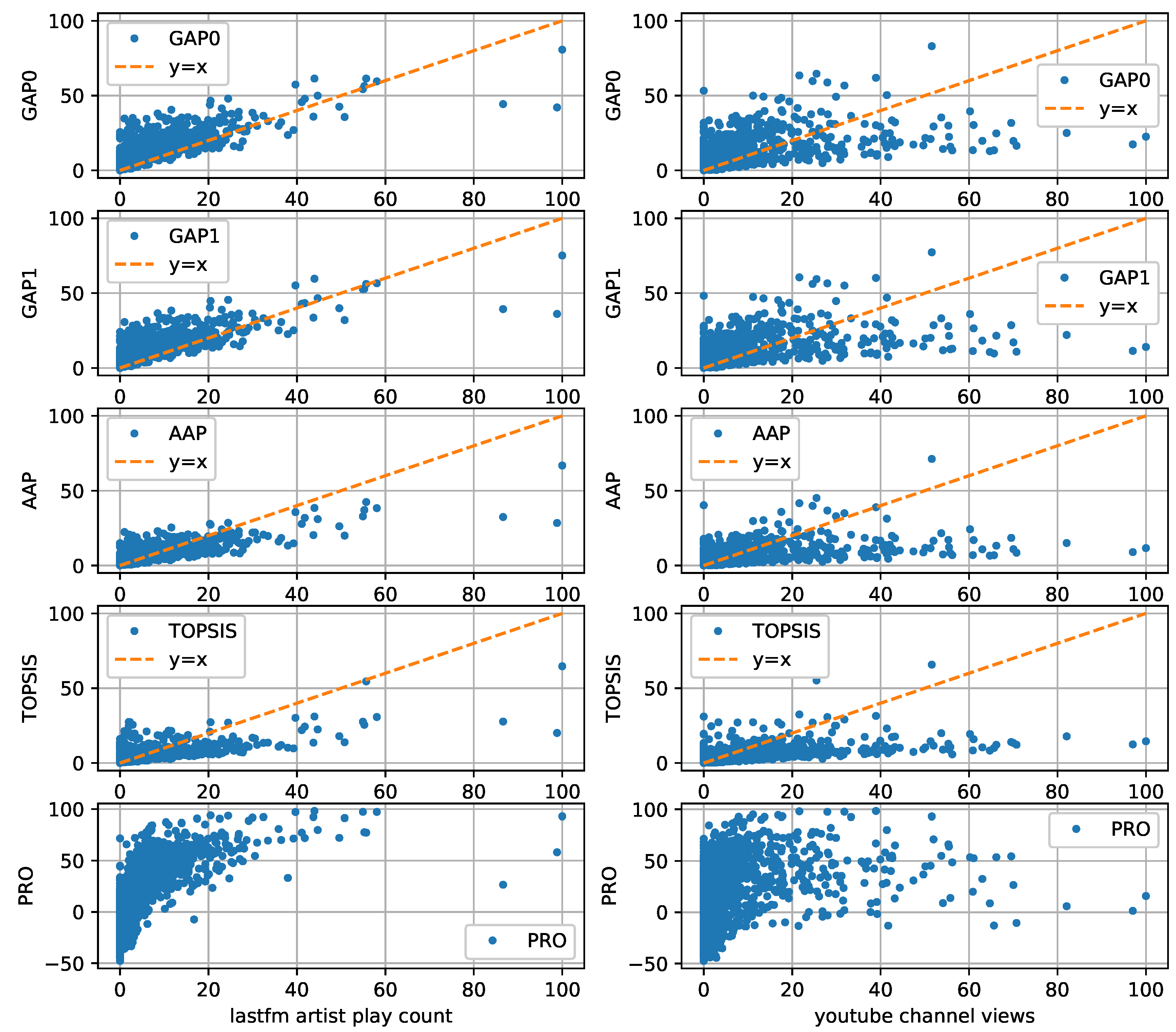
Figure 2, we compare the values of all aggregation methods with the normalized Last.fm artist plays and YouTube channel views with regard to a certain date, being 2 April 2019, using scatter plots. Furthermore, in Table 3, we present the corresponding similarity measures: Pearson correlation ( r P ) and Mutual Information (MI) for the linear and non-linear interrelationship between the aggregation methods and the target variables. We also investigated if the best aggregation method differed significantly from the other methods, in terms of similarity to the target. The statistical significance of the differences was estimated as proposed in [21] (dependent overlapping variables) for Pearson correlation and using a randomization test (We denote by y R N the target variable, by x 1 R N and x 2 R N the under comparison aggregation methods, and by θ * = I ( x 1 , y ) I ( x 2 , y ) the test statistic, where I ( · ) is the mutual information. Considering an approach similar to the permutation test proposed in [22], the test statistic value θ r of the r th Monte-Carlo simulation was computed by the permuted data, which were obtained by pooling x 1 and x 2 and assigning N of them randomly sampled without replacement to the x 1 group. The rest were assigned to the x 2 group. We considered R = 1000 Monte-Carlo simulations for the computation of the p-values, which were then determined by Equation (3):
p v a l u e = | θ r θ * | R
where | · | denotes the cardinality of a set.) for mutual information. To the best of our knowledge, there are many parametric statistical tests for differences in Pearson correlation [23], yet none for differences in mutual information; thus, we opted for the randomization test. It was apparent, from the scatter plots of Figure 2 where the dots are more concentrated and from the correlation analysis of Table 3 where higher similarity scores are illustrated, that all aggregation methods were correlated with Last.fm artist plays to a much higher degree than with YouTube channel views. Thus, we finally chose Last.fm artist plays as the ground truth for our experiments. In Table 4, the similarity of the aggregation methods with Last.fm artist plays on 2 April 2019 is illustrated using all measures of similarity. The statistical significance of the corresponding differences was estimated by Zoo’s method [21] for Pearson correlation and also using the previously described randomization test for all measures of similarity.
In Table 5, the average similarity between Last.fm artist plays and the aggregation methods across time (from 1 July 2018 until 31 May 2019) is exemplified in terms of linear/non-linear correlation and rank correlation/distance. The results showed that GAP1 exhibited the best performance in three out of seven measures of similarity, while AAP in two, GAP0 and PRO in one each, and TOPSIS in zero. Furthermore, the statistical significance of the differences in average similarity was investigated for all similarity measures, using Student’s t-test and by correcting the p-values using the Bonferroni correction for multiple comparisons ( α = 0.05 ). (For each similarity measure, we conducted four comparisons (the best aggregation method vs. each of the rest), so 4 × 7 = 28 comparisons were considered, and the 28 corresponding p-values were modified through the Bonferroni correction).
Although the aggregation methods produced similar artist popularities and rankings (not many statistical significant differences were observed), the correlation analysis showed that GAP produced popularity values that were closer to the target than the other aggregation methods when considering the non-linear similarity measure of mutual information and not when considering the linear correlation. This indicated the advantage of GAP to capture more complex popularity patterns than the simple average, which produced higher values only in linear correlation. In terms of ranking, GAP exhibited less distance from the target’s ranking with regard to Spearman’s footrule and Kendall’s tau distance measures and more proximity to the target’s ranking with regard to Kendall’s tau. PRO approximated best the target’s artist ranking with regard to the Spearman correlation coefficient, and both GAP and AAP showed almost identical rankings with regard to overall rank overlap.
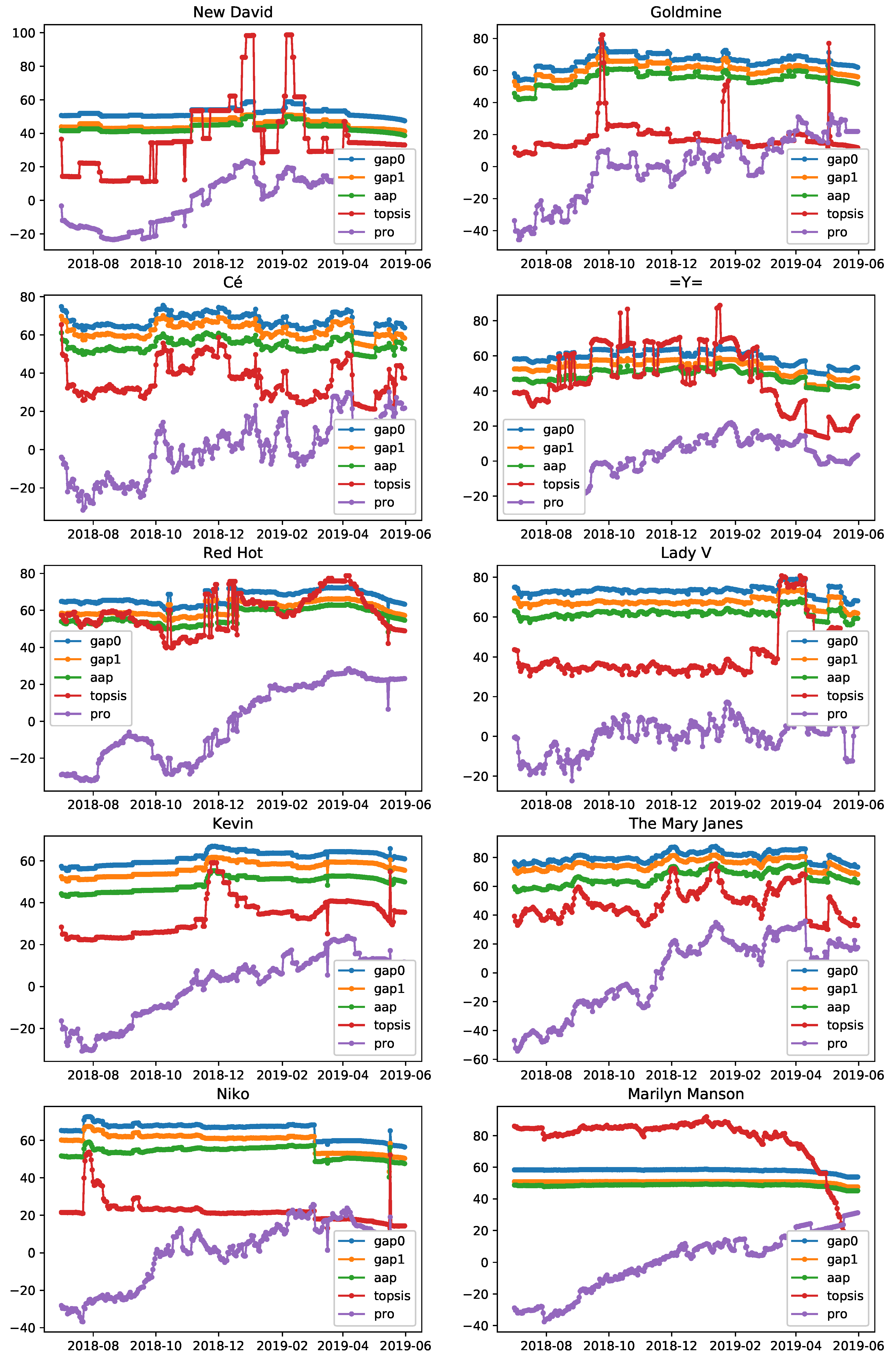
In Figure 3, we present the aggregation methods’ timelines for 10 popular artists with the highest discrepancy among the monitored popularity metrics. We focused on artists that exhibited differences in their popularity among different popularity metrics, because otherwise, the aggregation methods would provide the same information as the individual metrics and the comparison among them would not yield noteworthy conclusions. In order to select them, we first uncovered the set A of the 100 most popular artists on a certain date, being 1 April 2019, by sorting the sums of differences between each artist’s metric values and the maximum metric values in our dataset, as shown in Equation (4):
a r g s o r t i = 1 n m : , i , t 0 m a x ( m : , i , t 0 )
where n is the number of metrics, t 0 = 1 April 2019, m : , i , t 0 is the vector of normalized metric values for metric i, time t 0 , and all artists, and m a x ( v ) is the maximum value in vector v. Consequently, we employed Shannon entropy [24] as a measure of discrepancy on the distribution of normalized metric values per artist and selected the 10 artists of set A that exhibited the highest discrepancy, namely lowest entropy, as shown in Equation (5):
a r g s o r t E ( m ^ a , : , t 0 ) | a A
where m ^ a , : , t 0 is the vector of normalized metric values regarding artist a at time t 0 and E ( v ) is the Shannon entropy computed on vector v. The vector m ^ a , : , t 0 was divided by the sum of its elements in order to sum to one, prior to entropy calculation.
It was observed that these 10 artists retained high aggregated popularity values, in terms of GAP, despite the low level of popularity in some individual metrics, while AAP produced lower popularity values as a result of low popularity in some individual metrics. Furthermore, a more stable trajectory was exhibited by GAP0, GAP1, and AAP compared with TOPSIS and PRO, which were more volatile, which partly explained their inferior performance. The fact that GAP produced higher popularity values when the artist was popular in one or some metrics while not popular in the others was considered as a major advantage comparing to AAP. The reason for that was twofold: (a) first, because it was not common for artists to be popular in all platforms; they tended to be active mainly in one or some of them; and (b) second, because being popular in one or some platforms was sufficient for an artist to be characterized as popular in general.
In Table 6, we present a simulated example in order to showcase this advantage. It was observed that although in most metrics, a low popularity level was exhibited, being popular in Metric 4 enabled GAP to also exhibit a relatively high popularity estimate. On the contrary, AAP assigned a relatively low popularity estimate to the same entity. Finally, in Table 7, three cases of the artists of our dataset with metric values distributed as in the simulated case are exemplified, and the same conclusion was drawn again from these example cases.

4. Discussion

In this study, we proposed an aggregation method for popularity metrics that leveraged diverse sources of popularity information such as metrics derived from social media and streaming platforms. This was the first attempt to aggregate multiple popularity sources in the academic literature related to music information retrieval and admittedly yielded satisfactory results on the very useful task of summarizing the whole popularity picture of an artist. Its algorithm used geometrical shapes formatted by the individual metrics’ values of each entity, and it was found to outperform the most natural choice for metric aggregation, being a simple average, with respect to several measures of similarity between the computed metrics and reference data. Furthermore, the proposed aggregation method was robust even when the under study artist was popular only in some of the monitored popularity metrics. Finally, we should mention that our methodology could be extended for use in several other areas such as cinema and football in which actors and players will serve as entities and their social media accounts and other related factors (e.g., tickets/jerseys sold) as metrics. Future work will include the evaluation of all metric aggregation methods on other tasks, such as the prediction of individual metrics’ future values.

Author Contributions

Data curation, C.K. and M.S.; formal analysis, C.K.; funding acquisition, S.P. and I.K.; investigation, C.K.; methodology, C.K.; project administration, M.S., S.P., and I.K.; software, C.K. and M.S.; supervision, S.P. and I.K.; validation, C.K.; visualization, C.K.; writing, original draft, C.K.; writing, review and editing, C.K. and S.P. All authors have read and agreed to the published version of the manuscript.

Funding

This work is partially funded by the European Commission under Contract Number H2020-761634 FuturePulse.

Conflicts of Interest

The authors declare no conflict of interest. The funders had no role in the design of the study; in the collection, analyses, or interpretation of data; in the writing of the manuscript; nor in the decision to publish the results.

References

  1. Lee, J.; Lee, J.S. Music Popularity: Metrics, Characteristics, and Audio-Based Prediction. IEEE Trans. Multimed. 2018, 20, 3173–3182. [Google Scholar] [CrossRef] [Green Version]
  2. Almgren, K.; Lee, J.; Kim, M. Prediction of image popularity over time on social media networks. In Proceedings of the 2016 Annual Connecticut Conference on Industrial Electronics, Technology Automation (CT-IETA), Bridgeport, CT, USA, 14–15 October 2016; pp. 1–6. [Google Scholar]
  3. Nezhadbiglari, M.; Gonçalves, M.A.; Almeida, J.M. Early Prediction of Scholar Popularity. In Proceedings of the 16th ACM/IEEE-CS on Joint Conference on Digital Libraries, Newark, NJ, USA, 19–23 June 2016; pp. 181–190. [Google Scholar]
  4. Pera, M.S.; Ng, Y.K. A group recommender for movies based on content similarity and popularity. Inf. Process. Manag. 2013, 49, 673–687. [Google Scholar] [CrossRef]
  5. Liu, Z.; Dong, M.; Gu, B.; Zhang, C.; Ji, Y.; Tanaka, Y. Impact of item popularity and chunk popularity in CCN caching management. In Proceedings of the 2016 18th Asia-Pacific Network Operations and Management Symposium (APNOMS), Kanazawa, Japan, 5–7 October 2016; pp. 1–6. [Google Scholar]
  6. Ozer, M.; Sapienza, A.; Abeliuk, A.; Muric, G.; Ferrara, E. Discovering patterns of online popularity from time series. Expert Syst. Appl. 2020, 151, 113337. [Google Scholar] [CrossRef] [Green Version]
  7. Dwork, C.; Kumar, R.; Naor, M.; Sivakumar, D. Ranking aggregation methods for the web. In Proceedings of the 10th international conference on World Wide Web, Hong Kong, China, 1–5 May 2001; pp. 613–622. [Google Scholar]
  8. Chignell, M.; Tong, T.; Mizobuchi, S.; Delange, T.; Ho, W.; Walmsley, W. Combining Multiple Measures into a Single Figure of Merit. Procedia Comput. Sci. 2015, 69, 36–43. [Google Scholar] [CrossRef] [Green Version]
  9. Brans, J.P.; Vincke, P. A Preference Ranking Organisation Method: (The PROMETHEE Method for Multiple Criteria Decision-Making). Manag. Sci. 1985, 31, 647–656. [Google Scholar] [CrossRef] [Green Version]
  10. Yoon, K. A Reconciliation among Discrete Compromise Solutions. J. Oper. Res. Soc. 1987, 38, 277–286. [Google Scholar] [CrossRef]
  11. Grace, J.; Gruhl, D.; Haas, K.; Nagarajan, M.; Robson, C.; Sahoo, N. Artist Ranking Through Analysis of On-line Community Comments. In Proceedings of the 17th International World Wide Web Conference, Beijing, China, 21–25 April 2008. [Google Scholar]
  12. Schedl, M.; Pohle, T.; Koenigstein, N.; Knees, P. What’s hot? estimating country-specific artist popularity. In Proceedings of the International Society for Music Information Retrieval, Utrecht, The Netherlands, 9–13 August 2010. [Google Scholar]
  13. Schedl, M. Analyzing the Potential of Microblogs for Spatio-Temporal Popularity Estimation of Music Artists. In Proceedings of the IJCAI, Barcelona, Spain, 16–22 July 2011. [Google Scholar]
  14. Mesnage, C.; Santos-Rodriguez, R.; McVicar, M.; De Bie, T. Trend extraction on Twitter time series for music discovery. In Proceedings of the Workshop on Machine Learning for Music Discovery, 32nd International Conference on Machine Learning, Lille, France, 7–9 July 2015. [Google Scholar]
  15. Abel, F.; Diaz-Aviles, E.; Henze, N.; Krause, D.; Siehndel, P. Analyzing the Blogosphere for Predicting the Success of Music and Movie Products. In Proceedings of the 2010 International Conference on Advances in Social Networks Analysis and Mining, Odense, Denmark, 9–11 August 2010; pp. 276–280. [Google Scholar]
  16. Koenigstein, N.; Shavitt, Y. Song Ranking based on Piracy in Peer-to-Peer Networks. In Proceedings of the International Society for Music Information Retrieval, Kobe, Japan, 26–30 October 2009; pp. 633–638. [Google Scholar]
  17. Bellogín, A.; de Vries, A.P.; He, J. Artist Popularity: Do Web and Social Music Services Agree? In Proceedings of the Seventh International AAAI Conference on Weblogs and Social Media, Cambridge, MA, USA, 8–11 July 2013.
  18. Ren, J.; Shen, J.; Kauffman, R.J. What Makes a Music Track Popular in Online Social Networks? In Proceedings of the 25th International Conference Companion on World Wide Web, Montreal, QC, Canada, 11–15 April 2016; pp. 95–96. [Google Scholar]
  19. Kim, Y.; Suh, B.; Lee, K. #Nowplaying the Future Billboard: Mining Music Listening Behaviors of Twitter Users for Hit Song Prediction. In Proceedings of the First International Workshop on Social Media Retrieval and Analysis, Gold Coast, Australia, 11 July 2014; Association for Computing Machinery: New York, NY, USA, 2014; pp. 51–56. [Google Scholar]
  20. Koutlis, C.; Schinas, M.; Gkatziaki, V.; Papadopoulos, S.; Kompatsiaris, Y. Data-driven song recognition estimation using collective memory dynamics models. In Proceedings of the 20th International Society for Music Information Retrieval Conference (ISMIR), Delft, The Netherlands, 4–8 November 2019; pp. 368–375. [Google Scholar]
  21. Zoo, G.Y. Toward Using Confidence Intervals to Compare Correlations. Psychol. Methods 2007, 12, 399–413. [Google Scholar] [CrossRef] [PubMed]
  22. Venkatraman, E.S. A Permutation Test to Compare Receiver Operating Characteristic Curves. Biometrics 2000, 56, 1134–1138. [Google Scholar] [CrossRef] [PubMed]
  23. Diedenhofen, B.; Musch, J. cocor: A Comprehensive Solution for the Statistical Comparison of Correlations. PLoS ONE 2015, 10, e0121945. [Google Scholar] [CrossRef] [PubMed] [Green Version]
  24. Shannon, C.E. A mathematical theory of communication. Bell Syst. Tech. J. 1948, 27, 379–423. [Google Scholar] [CrossRef] [Green Version]
Figure 1. Example of the computation of Geometric Aggregation of Popularity (GAP) metrics for the artist “The Rasmus” on 2 April 2019. Version (a) GAP0 and (b) GAP1. The following abbreviations are used: DAF, Deezer Artist Fans; FF, Facebook Fans; FM, Facebook Mentions; LAL, Last.fm Artist Listeners; LAP, Last.fm Artist Plays; SCAF, Soundcloud Artist Followers; SPAF, Spotify Artist Followers; SAP, Spotify Artist Popularity; TUF, Twitter User Followers; TUL, Twitter User Listed; YCS, YouTube Channel Subscribers; YCV, YouTube Channel Views.
Information 11 00323 g001
Figure 2. Scatter plots of Average Artist Popularity (AAP), GAP0, GAP1, TOPSIS, and Preference Ranking Organization (PRO) vs. Last.fm play counts (Left) and YouTube channel views (Right). Each dot represents an artist.
Information 11 00323 g002
Figure 3. Timelines of aggregated artist popularity computed by GAP0, GAP1, AAP, TOPSIS, and PRO, for 10 artists with high discrepancy in their popularity as expressed by the monitored individual metrics.
Information 11 00323 g003
Table 1. Ground truth and evaluation methods for artist popularity proposed in the research literature.
PaperEvaluation Method
Grace et al. 2008One popularity proxy evaluated by user study (sentiment of comments on artists’ pages in MySpace)
Koenigstein and Shavitt 2009One popularity proxy compared with the Billboard Hot 100 (P2P search queries from Gnutella)
Schedl et al. 2010Four popularity proxies compared pairwise (page counts Google-Exalead, Twitter posts, shared folders in Gnutella P2P, Last.fm play counts)
Schedl 2011One popularity proxy compared with Last.fm’s charts (number of tweets with regard to an artist)
Bellogin et al. 2013Four popularity proxies compared pairwise (EchoNest score, Spotify popularity, number of Last.fm play counts, number of clicks related to an artist from Bit.ly)
Kim et al. 2014One popularity proxy used to predict Billboard ranks (number of tweets)
Table 2. Web-based sources and metrics for artist popularity.
SourceMetric
Deezerartist fans
Facebookfans
mentions
Last.fmartist listeners
artist plays (the last 30 days)
ine Soundcloudartist followers
Spotifyartist followers
artist popularity
Twitteruser followers
user listed
YouTubechannel subscribers
channel views (the last 30 days)
Table 3. Pearson correlation ( r P ) and Mutual Information (MI) measures of similarity between the target variables (Last.fm artist plays, YouTube channel views) and the aggregation methods (AAP, GAP0, GAP1, TOPSIS, PRO) on 2 April 2019. With bold letters, we denote the best value per similarity measure and target variable. With the exponents, we denote the best similarity scores for which their difference from the 2nd, 3rd, 4th, or 5th best, respectively, is statistically significant (95% confidence). For r P , the first number in the exponent concerns Zoo’s method, while the second concerns the randomization test.
Last.fmYouTube
r P MI r P MI
GAP00.80860.71500.56550.5084 5
GAP10.80730.7164 4 0.54960.4990
AAP0.8287 2 , 4 0.70980.55390.5046
TOPSIS0.75310.63810.5908 2 , 5 0.4912
PRO0.63250.66290.42620.4484
Table 4. Measures of similarity between the target variable (Last.fm artist plays) and the aggregation methods (AAP, GAP0, GAP1, TOPSIS, PRO) in 2 April 2019. With bold, we denote the best performance per measure of similarity (column). With the exponents, we denote the best similarity scores for which their difference from the 2nd, 3rd, 4th, or 5th best, respectively, is statistically significant (95% confidence). For r P , the first number in the exponent concerns Zoo’s method, while the second concerns the randomization test. ORO, Overall Rank Overlap; F, Spearman’s Footrule distance.
r S r P MIOROF r K K
GAP00.86090.80860.71500.81950.15260.77910.1105
GAP10.86240.80730.7164 4 0.81940.1523 5 0.7799 5 0.1101 5
AAP0.86050.8287 2 , 4 0.70980.81950.15260.77900.1105
TOPSIS0.83150.75310.63810.79380.17220.75130.1244
PRO0.8656 5 0.63250.66290.80690.15830.77430.1128
Table 5. Average similarity between the target variable (Last.fm artist plays) and the aggregation methods (AAP, GAP0, GAP1, TOPSIS, PRO) across time (from 1 July 2018 until 31 May 2019). With bold, we denote the best average performance per measure of similarity (column). With the exponents, we denote the best similarity scores for which their difference from the 2nd, 3rd, 4th, or 5th best, respectively, is statistically significant (95% confidence) after Bonferroni correction for multiple comparisons.
r S r P MIOROF r K K
GAP00.85410.80470.6948 4 0.81520.15680.77330.1134
GAP10.85560.80390.69210.81520.1564 4 0.7741 4 0.1129 4
AAP0.85380.8281 2 0.69300.8152 4 0.15670.77320.1134
TOPSIS0.82400.75690.62730.78920.17690.74520.1274
PRO0.8566 5 0.62290.63800.80310.16220.76780.1161
Table 6. Calculation of GAP0, GAP1, and AAP on a simulated entity with 4 monitored individual metrics, exhibiting high popularity in one metric and low in the others.
MetricPopularityGAP0GAP1AAP
10.1758.144.932.7
20.12
30.15
40.87
Table 7. Popularity scores as expressed by all individual metrics and aggregation methods GAP0, GAP1, and AAP for three artists of our dataset. The following abbreviations are used: DAF, Deezer Artist Fans; FF, Facebook Fans; FM, Facebook Mentions; LAL, Last.fm Artist Listeners; LAP, Last.fm Artist Plays; SCAF, Soundcloud Artist Followers; SPAF, Spotify Artist Followers; SAP, Spotify Artist Popularity; TUF, Twitter User Followers; TUL, Twitter User Listed; YCS, YouTube Channel Subscribers; YCV, YouTube Channel Views.
John LundvikRed HotDenz
DAF0.0450.0660
FF0.13100.156
FM0.14000.036
LAL0.1690.1090.135
LAP0.3580.0260.208
SCAF0.0170.2990.062
SPAF0.1630.0360.191
SAP0.8060.0200.755
TUF0.08900
TUL0.03400
YCS0.0800.6420.140
YCV0.0880.7000.261
GAP031.526.029.4
GAP127.923.325.9
AAP17.715.816.2

