Benchmark

A Controlled Benchmark of Video Violence Detection Techniques

Computer Science Department, Università degli studi di Bari “Aldo Moro”, 70121 Bari, Italy
*
Author to whom correspondence should be addressed.
Information 2020, 11(6), 321; https://doi.org/10.3390/info11060321
Submission received: 12 May 2020 / Revised: 1 June 2020 / Accepted: 5 June 2020 / Published: 13 June 2020

Abstract

:
This benchmarking study aims to examine and discuss the current state-of-the-art techniques for in-video violence detection, and also provide benchmarking results as a reference for the future accuracy baseline of violence detection systems. In this paper, the authors review 11 techniques for in-video violence detection. They re-implement five carefully chosen state-of-the-art techniques over three different and publicly available violence datasets, using several classifiers, all in the same conditions. The main contribution of this work is to compare feature-based violence detection techniques and modern deep-learning techniques, such as Inception V3.

1. Introduction

One of the most active researches in the computer vision field is analyzing the crowd’s behaviors. A crowd is defined as a group of people gathered in the same place. [1] Crowds differ according to the context, for example, the crowds inside a temple are different from those inside a shopping mall. The context in which the word “crowd” is used, indicates therefore the type of aggregation in terms of size, duration, composition, cohesion, and proximity of individuals to each other [1]. Analyzing these crowds is essential to prevent critical situations or control them before they degenerate. Crowd analysis helps in numerous ways:
  • Understanding crowd dynamics;
  • Allowing the development of crowd control systems;
  • Support designing and organizing public areas;
  • Improving animation models (e.g., for simulations and special effects creation in videogames design).
It uses processes such as recognition of individuals’ behavior, estimation of group density, and prediction of movements. The analysis should have the ability to differentiate a normal situation from an abnormal one, determining the nature of the event that is taking place in the scene, e.g., if violent or not.
To determine a certain type of event, it is necessary to develop algorithms that focus on the actions that belong to the event, removing those that are not part of it; it is necessary to take into account the occlusions that could exist, the context in which the event occurred, environmental conditions, and many other factors that affect certain behaviors [2].
This is a computationally intensive problem: The development of these systems leads to a computation of a large number of data. The technologies developed should ensure that the recognition of events is obtained in real time or near real time [3].
Among the events that can occur in crowded areas, there are some that are of particular importance. Some of them are theft, terrorism, aggression, panic, and other forms of violence. If crowds are not properly managed, this could undermine individuals’ safety, creating inconvenient and unpleasant situations, potential injuries, and, in the worst cases, deaths [4].
Thus, one of the most important problems in crowd behavior analysis is violence detection.
Videos play a fundamental role for today’s society, granting more security to big areas, where a large amount of people are expected to temporarily concentrate in limited areas. Increasing security in these areas is the main criteria behind the widespread use of video surveillance systems. Increasing security in these areas is the main criteria behind the widespread use of video surveillance systems. Actually, there are cameras installed in streets, shopping malls, temples, stadiums, and in many other contexts. However, the human eye cannot always predict where the situation is about to get of control: Even by using a top-of-the-range video surveillance system with multiple CCTV cameras, the human eye is not able to simultaneously check all of the monitors; thus, a computer-aided detection system is needed.
It is vital to prevent potentially harmful situations, and to take action as soon as possible. A system able to recognize violent actions among a crowd could be of immense help to the vigilance security team and contribute to restoring order before the situation deteriorates. Furthermore, there is a strong need for systems that could be easily and immediately integrated into already existing video surveillance cameras.
The aim of this work is benchmarking some of the methods already present in the state-of-the-art for Violence Detection in Video, on different and publicly available violence datasets over several classifiers, all in the same conditions. The selection of the techniques was based on the importance of the literature review, e.g., ViF is one of the firsts and most prominent techniques, while Motion Blob, IFV, and Haralick, instead, are often used as a comparison. In addition, the choice was based on accuracy, prediction time, implementation complexity, and new trends.
The paper is organized as follows:
Section 2 describes some publicly available datasets used in reviewed works. Section 3 sketches the techniques used in the reviewed works. At the end of the section, a summary table with cited works, features, and accuracies is provided for a quick glance. Section 4 presents the experimental design and the results, including summary tables that show the re-implemented works, the datasets, the accuracies, and per-frame time of execution. These tables are of extreme importance and represent a reference for future video violence detection systems. Conclusions and future work are presented in Section 5.

2. Datasets

In this section, the datasets used for experiments are described.

2.1. Violent-Flows-Crowd Violence/Non-Violence Dataset

It is a real-world database [5] of 246 videos, half of which contains violent acts scenes in crowded places, the other half consisting of non-violent scenes. The videos were taken from contexts such as roads, football stadiums, volleyball courts, ice hockey arenas, and schools. The videos were taken from YouTube. The shortest clip has a duration of 1.04 s, and the longest lasts 6.52 s. The average length of a clip is 3.60 s. The resolution is 320 × 240 p.

2.2. Hockey Fights Dataset

This database [6] is a set of 1000 videos extracted from NHL (National Hockey League) games, divided into 500 videos of violent scenes and 500 videos of non-violent scenes. The resolution of the videos is 360 × 288 p, and the frames per video are approximately 50. The task of this dataset aims for violence detection.

2.3. UCF 101 Dataset

Taken from YouTube, it is a realistic actions dataset [7] that includes 101 categories of actions. It showcases a great diversity, not only of actions, but also of camera movements, of objects differently positioned in the space, perspectives, and a variety of backgrounds and lighting conditions. It also includes 50 actions from different sports. The resolution of the videos is 320 × 240 p. The goal of this dataset is recognizing actions.

2.4. Hollywood2

This dataset [8] provides a set of 12 classes of human actions and 10 classes of scenes, distributed along 3669 video clips, with a total length of approximately 20.1 h. The various clips are scenes taken from 69 films.

2.5. Movies Dataset

This dataset [9] consists of 200 videos, 100 of which are fighting scenes taken from action movies. Non-violent scenes were taken from public action-recognition datasets. The videos do not have the same resolution. This dataset was created to be used for violence detection systems.

2.6. Behave Dataset

This dataset has 200,000 frames [10], with various scenarios, such as people walking, running, chasing each other, discussing in a group, driving, fighting, etc. The videos are captured at a rate of 25 frames per second. The resolution is 640 × 480 p. They are available in AVI format or in JPEG format.

2.7. Caviar Dataset

The CAVIAR dataset [8] was created to give a representation of different scenarios of interest. These include people who walk alone, who meet up with others, enter and leave shops, shop, fight, and exchange parcels in public areas.
It is made of two sets of videos filmed in two different scenarios: the entrance to the INRIA Lab and a shopping percent in Portugal.

2.8. UCSD Dataset

The UCSD dataset [11] involves videos of a crowded pedestrian walkway. The data are divided into two subsets, which correspond to two different scenes. The first, named “ped1”, contains clips of 158 × 238 pixels, representing groups of people walking back and forth toward the camera, with a certain degree of perspective distortion. The second, denoted with “ped2”, has a resolution of 240 × 360 pixels and depicts a scene where most pedestrians move horizontally.
A summary of the reviewed dataset are shown in Table 1.

3. Reviewed Works and Implementation Details

In this benchmark, the violence scene detection is referred to as a classification problem, where each frame or a sequence of frames in a time window is classified as violent or non-violent. This is a different problem from violence detection in videos, where the system identifies if and where the violence is taking place in the video. The classification is obtained by extracting certain features (or characteristics) from subsequent frames, as well as by using machine learning classifiers, such as support vector machines, etc.
In this section, 11 major features from several papers are reviewed and summarized.

3.1. ViF

Reference [5] considered how flow-vector magnitude changes over short frame sequences through time. The Authors used ViF (Violent Flow) descriptors. Given a sequence of frames S, an estimate of the optical flows between two consecutive frames is calculated for a short sequence of frames. This provides for each pixel p x , y , t , where t is the frame index, a vector ( u | x , y , t , v x , y , t ) who will be directed to another pixel in the next frame t + 1.
In Reference [5], only the magnitude of this vector is considered. This is shown in Equation (1).
m x , y , t = ( u 2 x , y , t + v 2 x , y , t )
Although optical flow vectors significantly encode temporal information, their magnitude is of arbitrary quantities: It depends on the resolution of the frame, on the different movements made in different spatiotemporal positions, etc. The significant measurements are obtained by comparing the movements’ magnitudes. The importance of these movements is compared with the previous frames.
For each pixel of each frame, we want a binary indicator, b x , y , t , which will reflect the change in magnitude between the frames. The binary indicator, b x , y , t , is shown in Equation (2).
2 b x , y , t = { 1       i f | m x , y , t m x , y , t 1 | θ 0       o t h e r w i s e
where the value to be exceeded θ is a threshold value set for each frame at the average quantity | m x , y , t m x , y , t 1 | . From here we obtain a binary map for each frame, f t , after which we calculate the average of the binary maps of each frame to obtain a single map with Equation (3).
b x , y ¯ = 1 T t b x , y , t
In its simplest form, this feature is a vector of frequencies of quantized values. If the “crowds” within the videos had stationary movement patterns, this feature is very discriminative. Essentially, however, different regions of the scene may have different characteristics and behaviors. For this reason, the map obtained is partitioned into non-overlapping M × N blocks, and the magnitude frequency changes are collected separately in each block. The distribution of magnitude changes in each of these blocks is represented by a histogram. These histograms are concatenated into a single vector that represents the ViF (Violent Flows) feature of the video.

3.2. OViF

OViF [12] was born to overcome the magnitude limitation of previously explained ViF technique by depicting information involving both motion magnitudes and motion orientations.
For computing OViF, optical flows are calculated between pairs of consecutive frames (Figure 1) [12] taken from the input video. The optical flow vector of each pixel can be represented as shown in Equations (4) and (5):
| V i , j , t | = ( V i , j , t x ) 2 + ( V i , j , t y ) 2
Φ i , j , t = a r c t a n ( V i , j , t y V i , j , t x )
where t is the t-th frame in the sequence of a video, and (i,j) indicate the positions of the pixels. After that, each optical flow map (therefore for each frame) is partitioned into non-superimposable M × N blocks. Thus, we have B sectors, and for each sector, there will be a histograms container. The magnitude of the optical flow | V i , j , t | is added to the container where the flow vector of the corner Φ i , j , t is positioned. These histograms will be concatenated into a single vector H, which is called the Histogram of Oriented Flow (HOOF) vector with X-dimensions, defined as shown in Equation (6):
X = M × N × B
The HOOF vector is used to obtain binary indicators computed as shown in Equation (7).
b x , t = { 1       i f | H x , t H x , t 1 | θ 0       o t h e r w i s e
Here, x is the x-th dimension of the feature vector H, and θ is the mean value of | H x , t H x , t 1 | ; x is included in [1,X]. This equation explicitly reflects magnitude changes and orientation changes for each region. The vector that will represent the average of the magnitude changes is defined in Equation (8).
b x , y ¯ = 1 T t b x , t
By the way, it would be the final OViF (Oriented Violent Flows) vector.

3.3. MoSIFT

The MoSIFT descriptor (Motion Scale–invariant feature transform) [13] finds and describes spatiotemporal points of interest on various scales.
Two main techniques are applied: the SIFT [13,14] algorithm for the identification of points of interest and the calculation of the optical flow based on the scale of the SIFT points of interest.
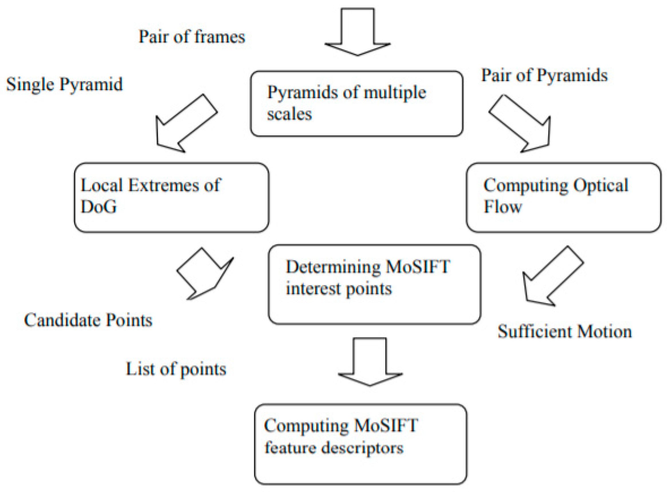
The steps for calculating the MoSIFT points of interest are summarized in Figure 2 [13]. First of all, the well-known SIFT algorithm is applied for finding points of interest in the space–time domain with (temporal) movements. SIFT points of interest are invariant at the representation scale; therefore, multiple scales are computed for a single image.
A Gaussian function is used as a kernel for the production of the image scale space. The entire scale space is divided into an octave sequence where each octave is divided into a sequence of intervals, and each interval is an additional scale of the frame. The number of octaves is determined by the size of the image. The weight relationship between two adjacent octaves is at the power of 2. The first interval in the first octave is the original frame. In each octave, the first interval is denoted as l ( x , y ) .
Thus, each interval is denoted as follows:
L ( x , y , k δ ) = G ( x , y , k δ ) I ( x , y )
where the convolution operator in x, y, and G ( x , y , k δ ) is a Gaussian smoothing function.
The difference of Gaussian images (DoG) is then computed by subtracting the adjacent intervals, as shown in Equation (10).
D ( x , y , k δ ) = L ( x , y , k δ ) L ( x , y , ( k 1 ) δ )
Once the DoG image pyramid has been calculated, the local (minimum/maximum) ends of the DoG images along adjacent scales are taken as points of interest. This is done by comparing each pixel of the DoG images with their eight neighbors on the same range and the nine corresponding neighboring pixels in each of the neighboring ranges. The algorithm searches through each octave in the DoG pyramid and detects every possible point of interest at different scales.
In identifying the points of interest of the MoSIFT algorithm, the optical flow is computed on two consecutive Gaussian pyramids. The optical flow is calculated at different scales, according to the scales derived from SIFT. An extreme point coming from the DoG pyramids can become a point of interest only if there is sufficient movement in the optical flow pyramid. Therefore, it is expected that a complicated action can be represented by a combination of a reasonable number of points of interest.
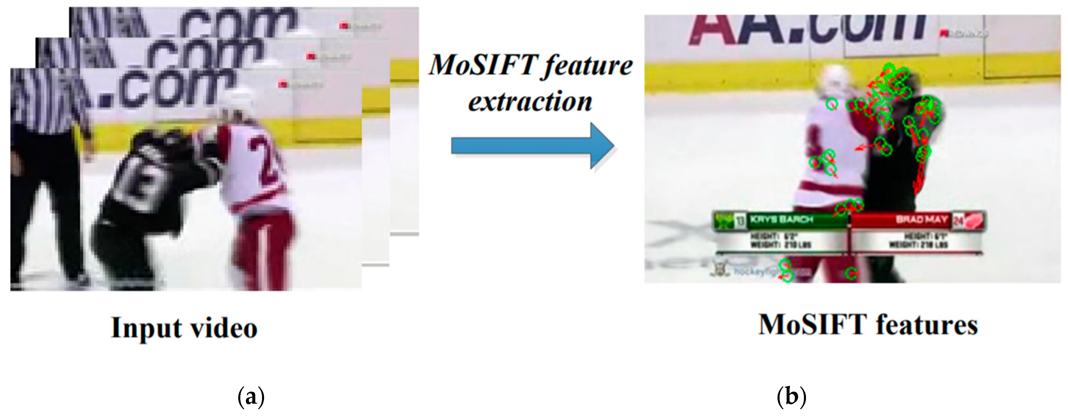
As long as a point of interest is characterized by a minimum of movement, the algorithm will extract this point as a MoSIFT point. The number of points of interest increases with the increase of movement in the sequence (Figure 3b).
MoSIFT points of interest are invariant to the type of scale in the space domain, while they are not invariant in the time domain. The invariance in the time domain could be obtained by calculating the optical flow of various scales in the time domain. Thus, given a video, the points of interest (MoSIFT) are calculated for each frame. Each point is a vector containing a histogram of optical flow HOF followed by a SIFT histogram, the size of this vector is 256 (128 HOF and 128 SIFT).

3.4. KDE, Sparse Coding, and Max Pooling

In Reference [13], the vector of size 256 of the MoSIFT points of interest is reduced to a vector of size 150, using the KDE (kernel density estimation) method. KDE is a nonparametric method to derive the probability density function (PDF). It is assumed that x 1 , x 2 , , x N are N independent data distributed in the same way taken from a random variable x. KDE infers the PDF of x by centering a K (x) kernel function at each point of x i , as shown in Equation (11).
f h ( x ) = 1 h N i = 1 N K ( x x i h )
where h > 0 is a smoothing parameter called band. For each j-th feature of the MoSIFT descriptor, the KDE method is used to obtain a PDF on the training data.
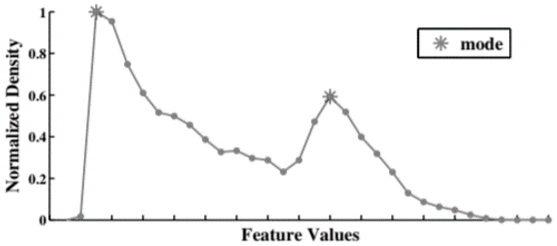
From the original size of 256 MoSIFT points, the PDF of each feature is estimated. Depending on the number of modes present (Figure 4), the 256 features are sorted in descending order. Thereafter, the first 150 features will be selected to form the reduced MoSIFT descriptor, creating, theoretically, a more efficient representation of the original descriptor.
In Reference [13], after the reduction of MoSIFT features through the KDE method, the sparse coding technique (Figure 5) is used to represent the actions produced in the videos.
Call X a set of MoSIFT feature vectors extracted from a video and previously reduced in size, and the sparse coding problem can be formulated as shown in Equation (12).
z = a r g Z R m i n k x N 1 2 X D Z l 2 2 + γ Z l 1
where Z = [ z 1 , z 2 , , z N ] , and z i is the “sparse representation” of the vector features x i . D = [ d 1 , d 2 , , d k ] is a pre-trained dictionary, and γ is a positive value to be adjusted to keep under control the exchange between the reconstruction error and the sparsity. The LARS-lasso method [15] is used to solve the previous equation in order to obtain the sparse-code set Z. This way, a video represented by X is converted into the corresponding representation in Z. After this, the analysis/recognition of the aforementioned video is done in the Z domain.
To capture the global statistics of the entire video, the max pooling technique is applied on the sparse-code representation Z, to obtain high-level features.
β = F ( Z )
In Equation (13), β is a vector of k dimensions, and F is a pooling function defined on each row of Z. The max pooling function is defined as shown in Equation (14).
β i = max { Z i , 1 , Z i , 1 , , Z i , N }
where β i is the i-th element of β, and Z i , j denotes the (i,j) -th element of the matrix Z.

3.5. HOA, HOP, HOD, and OE

Features from the work [16] are built over the intuition that the presence of large movement in the image is of paramount importance in violence recognition. The authors used motion blurs and the shifts in image content toward low frequencies as descriptors for building an efficient acceleration estimator for videos. The computed power spectrum depicts an ellipsoid. The orientation of the ellipsoid is perpendicular to the direction of the motion; thus, the acceleration happens in that direction. Their method in Reference [7] is based on detecting such an ellipsoid.
For each couple of consecutive frames present in the sequence of a video, the spectral power is calculated by using the 2D Fast Fourier Transform (in order to not incur into edge effects, a Hanning window is applied before calculating the FFT).
Given the spectral images Pi−1 and Pi, image C is obtained as shown in Equation (15).
C = P i P i 1
When there are no changes between the frames, the spectral powers will be equal, and C will have a constant value. When there are movements between frames, in image C, it is possible to observe an ellipse, as in Figure 6.
The identification of the ellipses can be carried out by using the Radon transform [17], with which images are projected along the lines with different orientations. After calculating the transform, its vertical projection is obtained and normalized to the maximum value 1. When there is an ellipse in image C, this projection will show a crest, which will represent the major axis of the ellipse. The kurtosis, K, of this projection is taken to estimate the acceleration of the action in the scene.
Kurtosis itself could not be used as a measure, because it is obtained from a normalized vector. Thus, the average power P of the image C is also calculated and taken as an additional feature. Deceleration is considered to be an additional feature, and it can be obtained by exchanging consecutive frames in the calculation of image C and by applying the same algorithm described for acceleration.
The acceleration, deceleration, and power vectors calculated along the frames of a video are respectively represented by histograms that are called HOA (Histogram of Acceleration), HOD (Histogram of Deceleration), and HOP (Histogram of Power).
An additional feature called Outer Energy (OE) is calculated. When the background is relatively uniform and the spacing is small, the estimate of global movement may still fail. The Hanning window [16] restricts operations by applying them only to the internal parts of the image. It is reasonable to assume that, when the movement is global, changes in the external parts of the image will be relatively equal to those of the internal parts of the image; from this concept, the Outer Energy is introduced as in Equation (16):
O x , y , t = | f x , y , t f x , y , t 1 | ( 1 H x , y ) M N
The average and the standard deviation of the Outer Energy are taken as additional features.

3.6. ConvLSTM Network

The deep neural network presented in work [18] uses AlexNet architecture as a CNN model, pretrained on the ImageNet dataset, in combination with an LSTM for extracting frames in the space–time domain. Convolutional Neural Networks (CNN) are networks capable of extracting spatial features. Convolutional layers are trained to extract hierarchical features. Instead of inserting frames as they are, the difference between adjacent frames is taken as input. Once all the images have been inserted, the hidden states of the ConvLSTM contain the final representation of the video (in the space–time domain), which will pass through a series of fully connected layers, where it will finally be classified as violent or non-violent.

3.7. Extraction of OHOF from Candidate Regions

The Gaussian Mixture Models (GMM) is adopted for the production of candidates as violent regions with movement features extracted from the information on the magnitudes of the optical flow vectors; this method is called Gaussian Model of Optical Flow (GMOF) [19,20].
Unlike GMM, GMOF aims to determine anomalies in movement rather than in pixels. A background model is constructed by using the optical flow magnitudes in a defined image. The frames of a video are partitioned into n × n grids (each cell with a size of 4 × 4), with an overlap of 50%.
For each grid, the average of the magnitudes of the optical flow vectors is calculated, and the Gaussian model is updated and constructed.
For each time, t, we denote the history of the set of movement features (in terms of speed of magnitude) of a cell, such as {m1, m2, ..., mt}, which is modeled by a mixture of K Gaussian distributions. Given the optical flow range (u, v) of each pixel, the magnitude speed, m, for a 4 × 4 cell can be calculated as in Equation (17).
m = 1 16 u 2 + v 2
The probability of observing cell p is calculated as in Equation (18).
p ( m ( p ) , t ) = k = 1 k w k ( t ) g ( m ( p ) , μ k ( t ) , σ k 2 ( t ) )
where K is the number of distributions (set of three distributions in this case); w k ( t ) is the magnitude of the k-th GMM distribution at the time, t; μ k ( t ) and σ k 2 ( t ) are the mean and the covariance of the k-th Gaussian distribution; and g is a Gaussian function of probabilistic density.
At time t = 1, µ = m and σ = m (p) are initialized, where m (p) is the average value of the optical flow magnitude of the whole image. Based on the persistence and variance of each Gaussian distribution, it is determined which of the distributions can be associated with the crowd model. This can be solved by Equation (19).
m ( p ) μ n σ
If this equation is satisfied, the distribution parameters combining the new observation are updated as defined in Equation (20).
w k ( t + 1 ) = ( 1 a ) w k ( t ) + a
μ k ( t + 1 ) = ( 1 β ) μ k ( t ) + β m ( p )
σ k 2 ( t + 1 ) = ( 1 β ) σ k 2 ( t ) + β ( μ k ( t ) m ( p ) ) 2
where α and β are, respectively, the preset value of weight-learning and the value of mean/variance-learning. A low weight-learning value indicates that new movement features will be slowly incorporated into the model.
For distributions that are not associated, the weight will be updated as in Equation (23).
w k ( t + 1 ) = ( 1 a ) w k ( t )
While the mean and variance will remain unchanged, if that equation is not satisfied, the Gaussians will be ordered by the value of w k ( t ) / α , which will be increased proportionally to the increasing of the distribution evidence and the decreasing of the variance. After recalculating the GMM, the one with the greatest probability is taken.
Finally, candidate regions are determined as violent through the formulation presented in Equation (24).
a r g m i n ( k = 1 C m ( p ) > T t h r e s h )
where C denotes the number of satisfied distributions, and Tthresh is the verification measure of the candidate regions as violent, which takes the best distributions before a certain portion. If the inequality is satisfied, the region will be marked as violent; otherwise, it will not be. If Tthresh is small, the crowd model will be unimodal; otherwise, with a large Tthresh, a multimodal distribution will be included in the model.
The violent action verification algorithm contains two main aspects:
  • A multiscale scanning window used to search for violent events in the candidate regions;
  • The OHOF feature is extracted for each area of the image covered by the scanner window, to distinguish violent from non-violent actions.
The multiscale scanning window algorithm presented in work [10] operates in the following way:
As long as there are frames to analyze, we follow five steps:
  • Step 1: Scanning windows are built with three types of scales: 72 × 72, 24 × 24 and 8 × 8.
  • Step 2: Scroll the images through multiple scales with steps of 8 pixels at a time.
  • Step 3: If the scanning window crosses more than half of the candidate regions as violent regions, then skip to Step 4; otherwise, go back to Step 2.
  • Step 4: Update the candidate regions with the regions crossed by the scanning windows, and mark them as violent regions.
  • Step 5: Sample the new candidate regions as violent by using the method in work [10], and go back to Step 2.
The OHOF descriptor is extracted in the following way:
First, the optical flow orientation histogram is constructed by arranging the bins, adding contextual information, and normalizing everything.
The optical flow is computed with the Lucas–Kanade method [10]. For each pixel, two orientations of magnitudes are calculated, denoted as Fx and Fy, expressed using polar coordinates, as shown in Equation (25).
{ F x 2 F y 2 θ = a r c t a n F x F y
After, a histogram is constructed with 16 orientations of candidate regions as violent. Next, the bins of the resulting histogram are adjusted, keeping the orientations with the values of gradients larger than Tthresh, and ordering the bins of the histogram in descending order, according to their values. This is to make OHOF independent of the rotation of the scene. Later, contextual information is added. Histograms from six previous frames are added to the descriptor for robust performance. Therefore, the entire descriptor is 16 × 7 = 112 in size. Finally, the histogram is normalized, in order to resolve disturbances generated by small variations in light and eliminating the difference in the size of the regions on all the optical flow images of the video.

3.8. Improved Fisher Vector with Boosting and Spatiotemporal Information

The Improved Fisher Vectors (IFV) [6] is a video encoding technique which pools local features in a global representation. Local features are described as the magnitude of deviation from the GMM generative model.
The representation of the IFV in Reference [6] is in vector of gradients G λ x , which are firstly normalized with power normalization, and later with the L2 norm.
Given P as a set of T trajectories extracted from a video, pt is thus a feature point detected at a spatial position in a frame C. The position of a center of a trajectory is normalized, so that the size of the video does not significantly change the magnitude of a feature position vector. Once the positions of the local features are represented in a normalized way, unity-based normalization is also used to reduce the influence of the motionless regions at the edges of a video. Taken for the vector pt are the minimum and maximum values of the i-th dimension among all the vectors of normalized positions of the video extracted from the training videos.
The calculated vectors are incorporated into the IFV model; therefore, the videos can be represented by using both local descriptors and spatiotemporal positions. Assuming that the covariance matrices are diagonal, the various G vectors are then calculated. The new implementation of the Improved Fisher Vector is the vector of the G gradients normalized with the power normalization and then by the L2 norm.
In the last part of feature extraction, a sliding time window is scrolled. It evaluates the video subsequences as the locations and scales vary. Therefore, to speed up the detection frameworks, the IFVs are reformulated, and the data structure of the table of the summed area is used, so that the IFVs are calculated for features by time segments only once. Finally, by applying the power normalization, and then from the L2 standard, we obtain the vector of the gradients. However, unlike the original IFV, this boosted IFV can be used directly with data structures such as tables of summed areas and KDD trees. To avoid unnecessary weighting on the mathematical formulation, we refer to the original paper in Reference [6].

3.9. Haralick Feature

The method proposed by Reference [2] was built based on Haralick features, which describe the textures by using statistics derived from the co-occurrence of the gray levels. These features are calculated for each frame, in order to monitor how they change over time. Haralick features are extracted from a gray level co-occurrence matrix (GLCM), which is generated by counting the intensity of gray levels found in an image given a linear spatial relationship between two pixels. The spatial relationship is defined by the pair (θ, d), and then combined with the GLCM matrix. This is typically used to obtain rotational invariance by using a set of orientation parameters, typically eight directions, spaced by π/4 radians.
The number of gray levels Ng represents the number of unique intensity values present in an image. The Haralick features are therefore calculated:
  • Second Angular Moment:
    i , j = 0 N g 1 P i , j 2
  • Contrast: The following is an example of an equation:
    i , j = 0 N g P i , j ( i j ) 2 ( N g 1 ) 2
  • Homogeneity:
    i , j = 0 N g 1 P i , j 1 + ( i j ) 2
  • Correlation:
    [ i , j = 0 N g 1 P i , j 2 [ ( i μ i ) ( j μ i ) ( σ i 2 ) ( σ i 2 ) ] ] + 1 2
  • Dissimilarity:
    i , j = 0 N g 1 P i , j 2 i j 1 N g 1
    where Pi,j refers to the (i,j)-th pixel in the GLCM. Previous Equations (27)–(30) have been modified to give a value between [0, 1]. For an x sequence, we will have a series of values that will represent it. Each x sequence is represented with a vector of length 4 containing a statistical summary of Haralick features, and each vector is composed of arithmetic mean, standard deviation, asymmetry, and inter-frame uniformity (IFU).
  • Asymmetry:
    E ( x μ ) 3 σ 3
  • IFU:
    | y | 2 ( T 1 ) 1 ( T 1 ) 1
Equation (32) represents the similarity measure of adjacent samples in the ordered time data. It is expressed as the resized L2 norm of the sequence y; this sequence is formed by taking the absolute difference between the adjacent samples in the sequence x. The sequence y is normalized before being input to Equation (7). IFU returns a value in the range [0, 1], where 0 represents non-uniformity and 1 represents uniformity that changes over time. Before applying the above method, each frame is divided into N × M non-overlapping subregions.

3.10. Blobs Motion Features

Authors in Reference [20] proposed a technique called blobs motion features, where features extracted from motion blobs are used to discriminate fight and non-fight sequences. The method is not very accurate, but it is significantly faster than others, making it possible to integrate it into common surveillance systems.
The algorithm for extracting the blobs features can be described in the following steps:
(1)
Given a sequence of frames, each frame is converted into its grayscale, as in Equation (33):
S ( s ) = I t ( x , y )
(2)
Take It−1 (x, y) and It (x, y), which will be two consecutive frames at time t−1 and t, and the absolute difference of the two frames is given in Equation (34).
E t ( x , y ) = | I t 1 ( x , y ) I t ( x , y ) |
where (x, y) represents the position of a pixel in a frame.
(3)
This new matrix is transformed into the quantized binary form, using a threshold h, as shown in Equation (35):
F t ( x , y ) = { 1       i f E t ( x , y ) > 255 h 0 ,       o t h e r w i s e
where 0 < h < 1 can be chosen arbitrarily.
(4)
It is necessary to search for each blob in the image Ft (x, y). For each image Ft (x, y), some of the blobs are selected from which other information will be extracted. The selection will be made on the basis of the blob’s area.
(5)
The blob area (Aa,t) is defined as in Equation (36):
A a , t = x = 1 N y = 1 M B a , t ( x , y ) a
where a = 1, 2, …, K. K is the number of blobs for each Ft (x, y).
(6)
Centroids are also calculated as in Equation (37):
C X c , t = x = 1 N B c , t ( x , y ) x x = 1 N B c , t ( x , y ) = x = 1 N B c , t ( x , y ) x N C Y c , t = x = 1 N B c , t ( x , y ) y x = 1 N B c , t ( x , y ) = x = 1 N B c , t ( x , y ) x N
where c = 1, 2 … K.
(7)
Compute the Euclidean distance between two blobs’ centroids.
(8)
Compactness is used to estimate the shape of the blobs (circular or elliptical). It is defined as in Equation (38):
C c o , t = P c o , t 2 A c o , t
where co = 1, 2, …, K. P p , t is defined as in Equation (39):
P p , t = x = 1 N y = 1 M G p , t ( x , y ) P
where p = 1, 2, ..., K, and (Gp,t (x, y)) is the Sobel operator that is applied to determine the edges on Bb,t (x,y). The area, the centroids, the distance between the centroids, and the compactness of the blobs are taken as features and linked in a single vector (which will represent the video), which will then be analyzed by the classification algorithm.

3.11. Violence Detection with Inception V3

In this experimentation, it was decided to use Inception V3 deep neural network [21] for the classification of violent/non-violent videos.
The idea was to train a CNN on video frames taken from a dataset. The Inception V3 architecture was modified by adding four fully connected layers with sigmoid activation function, to perform binary classification.
The classification of the frame is a score ranging from 0 to 1, so if the frame belongs to the interval [0, 0.5], it is considered “Violent”. Vice versa, if it belongs to the interval [0.5, 1], the frame is recognized as “Non-Violent”. A video is classified as “Violent” if the average of the frames’ scores is ≤0.5; vice versa, if the average is >0.5, the video is considered “Non-Violent”.
A pretrained Inception V3 network was used. The network was pretrained on the ImageNet dataset. Several studies have shown that networks trained on this dataset have a better generalization ability and provide better results in tasks such as action recognition.
Four fully connected layers (Figure 7) were inserted in sequence. Respectively, the first three of 512, 256, and 100 units were used as added layer, and the last one as the classification layer, with a single neuron. Each layer has the activation function ReLU (the green block) and is alternated by a Dropout layer (blue block) with a value of 0.5. After the last fully connected layer, a “sigmoid” activation layer was inserted. This setting was defined after a series of tests, with the aim of not allowing the network to overfit and to obtain better results. The Adam [22] algorithm with learning rate 0.001 was used as the optimization algorithm.
Follows two summary tables. Table 2 reassumes each feature analyzed, their reference works and a brief description. Table 3, instead, reassumes each feature accuracy and their reference work with respect to several classifiers.

4. Experiments Setup and Results

From the previous 11 techniques, five techniques were selected, re-implemented, and tested in same conditions. The following techniques were selected based on the importance from the literature review, e.g., ViF was one of the first and most important techniques, while Motion Blob, IFV, and Haralick were often used for comparison. In addition, the choice was also performed based on accuracy, prediction time, implementation complexity, and new trends.
  • ViF;
  • Motion Blobs;
  • Inception V3;
  • Haralick;
  • Improved Fisher Vector.
For each video dataset, 70% of the videos were used for training, and the remaining 30% for testing. For Inception V3, simple data augmentation, such as rotation, shifting, and padding, was used to increase data within the training set. Moreover, a batch size of 32 was used. Each frame was resized to 150 × 150 pixels.
For the evaluation of each system, the k-fold cross-validation technique was used with k = 5, as used in other state of the art articles. For the Motion Blobs system, the value k = 10 was also used for the comparison of the system constructed with the respective reference article [21].
Random Forest algorithm was used with 50 trees, to avoid overfitting. The SVM used is a linear SVM with C = 1 to avoid overfitting. The experimental results are shown in Table 4.
From the results shown in Table 4, it is possible to see that Inception V3 outperforms all reviewed methods. It was expected to see higher results for the Haralick feature, as indicated in Reference [2], but that did not happen. This is probably due to the different training/test separation ratio with respect to the original paper.
It is important to focus also on the computational cost (the execution time) of the prediction algorithms. This is a key factor when it comes to real-time violence detection.
As it is possible to observe from Table 5, the best trade-off between accuracy and prediction time is still Inception V3, but when it comes to real-time violence detection system, especially if deployed in embedded systems, the Improved Fisher Vector is faster, with a relatively high level of accuracy.

5. Conclusions and Future Work

In this paper, five state-of-the-art violence detection techniques, over three different and publicly available violence datasets, using several classifiers, were reimplemented and tested, all in the same conditions. The main contribution of this work is to compare feature-based violence detection techniques and modern deep-learning techniques, such as Inception V3. The techniques were selected based on the importance from the literature review, e.g., ViF was one of the first and important techniques, while Motion Blob, IFV, and Haralick were often used for comparison. In addition, the choice was also performed based on accuracy, prediction time, implementation complexity, and new trends.
As shown in Table 3, the Inception V3 system turned out to be better than the other systems implemented, from the accuracy perspective. However, the training time of this system, compared to the others, proved to be more expensive.
This depends a lot on the number of frames used for the training. In fact, although the Violent-Flows-Crowd dataset and the Movies dataset had, more or less, the same number of videos, the first one needed more time to be analyzed, and despite this, its accuracy was lower than that of the Movies dataset. This is because the Violent-Flows-Crowd dataset presents many occlusions within the videos, like rapid camera movements and low frame quality, which do not help the algorithm to properly understand what is happening in the scene.
The Movies dataset, on the other hand, was the easiest to train and had the best accuracy among the three datasets selected for testing. This was because it presented much more readable scenes, since the videos were taken from films and therefore the image quality is better and the actions that are performed are clearer and less frenetic giving the possibility to the systems to easily distinguish violent videos from non-violent ones.
The longest training time was achieved with the Hockey dataset, with about 10 h of training, being the largest of the three datasets. The Hockey dataset is the one that best lends itself to the problem of identifying violent actions through video surveillance cameras, being composed of videos in which the context is always the same, but the people and actions of these change over time.
The results of the Inception V3 system are in line with the state-of-the-art. This system has also another advantage over other techniques, namely the possibility of being able to classify videos by selecting an arbitrary number of frames, being the neural network trained on spatial and non-temporal features, making the classification faster in terms of time (however at the expense of less reliability in the classification of videos).
Inception V3 and other deep-learning techniques, with the right equipment, can be used in real time and are applicable to video surveillance cameras, to allow an improvement also for people to feel safer and more secure. A good accuracy, by the way, was also achieved by Improved Fisher Vector. This technique is more suitable for low-demand embedded devices: we imagine this technique to be compiled and integrated into hardware, performing real-time violence detection in all of those scenarios where an internet connection is not present (limited capabilities of sending data to server for cloud GPU computation) and mounted, for example, on a mobile platform, or simply encoded directly inside cameras or mobile chips, for instant-on violence detection systems.
Our suggestion, for future researches, is to focus on deep-learning techniques in terms of both accuracy and prediction time. It could be interesting to see how specialized deep neural network models, trained on one particular dataset, such as for example the Movies dataset, performs when tested on other datasets or in real scenarios.

Author Contributions

Conceptualization, D.I. and G.P.; Data curation, V.D., N.C. and L.S.; Investigation, D.I., V.D., N.C., G.P. and L.S.; Methodology, D.I., V.D., G.P. and L.S.; Software, V.D., N.C. and L.S.; Supervision, D.I. and G.P.; Visualization, V.D. and L.S.; Writing—original draft, D.I. and V.D.; Writing—review & editing, V.D. and D.I. project administration, D.I.; funding acquisition, D.I. All authors have read and agreed to the published version of the manuscript.

Funding

This work was supported by the Italian Ministry of Education, University and Research within the PRIN2017—BullyBuster project—A framework for bullying and cyberbullying action detection by computer vision and artificial intelligence methods and algorithms. CUP: H94I19000230006.

Conflicts of Interest

The authors declare no conflict of interest.

References

  1. Afiq, A.; Zakariya, M.; Saad, M.; Nurfarzana, A.; Khir, M.; Fadzil, A.; Jale, A.; Witjaksono, G.; Izuddin, Z.; Faizari, M. A review on classifying abnormal behavior in crowd scene. J. Vis. Commun. Image Represent. 2019, 58, 285–303. [Google Scholar] [CrossRef]
  2. Lloyd, K.; Rosin, P.L.; Marshall, D.; Moore, S.C. Detecting violent and abnormal crowd activity using temporal analysis of grey level co-occurrence matrix (GLCM)-based texture measures. Mach. Vis. Appl. 2017, 28, 361–371. [Google Scholar] [CrossRef] [Green Version]
  3. Wilk, S.; Kopf, S.; Effelsberg, W. Video composition by the crowd: A system to compose user-generated videos in near real-time. In Proceedings of the 6th ACM Multimedia Systems Conference, Portland, OR, USA, 18–20 March 2015; pp. 13–24. [Google Scholar]
  4. Pujol, F.A.; Mora, H.; Pertegal, M.L. A soft computing approach to violence detection in social media for smart cities. Soft Comput. 2019, 1–11. [Google Scholar] [CrossRef]
  5. Hassner, T.; Itcher, Y.; Kliper-Gross, O. Violent flows: Real-time detection of violent crowd behavior. In Proceedings of the 2012 IEEE Computer Society Conference on Computer Vision and Pattern Recognition Workshops, Providence, RI, USA, 16–21 June 2012; pp. 1–6. [Google Scholar]
  6. Bilinski, P.; Bremond, F. Human violence recognition and detection in surveillance videos. In Proceedings of the 13th IEEE International Conference on Advanced Video and Signal Based Surveillance (AVSS), Colorado Springs, CO, USA, 23–26 August 2016; pp. 30–36. [Google Scholar]
  7. Deniz, O.; Serrano, I.; Bueno, G.; Kim, T.-K. Fast violence detection in video. In Proceedings of the 2014 International Conference on Computer Vision Theory and Applications (VISAPP), Lisbon, Portugal, 5–8 January 2014; pp. 478–485. [Google Scholar]
  8. Ribeiro, P.C.; Audigier, R.; Pham, Q.-C. RIMOC, a feature to discriminate unstructured motions: Application to violence detection for video-surveillance. Comput. Vis. Image Underst. 2016, 144, 121–143. [Google Scholar] [CrossRef]
  9. Ditsanthia, E.; Pipanmaekaporn, L.; Kamonsantiroj, S. Video representation learning for CCTV-Based violence detection. In Proceedings of the 3rd Technology Innovation Management and Engineering Science International Conference (TIMES-iCON), Bangkok, Thailand, 12–14 December 2018; pp. 1–5. [Google Scholar]
  10. Zhang, T.; Yang, Z.; Jia, W.; Yang, B.; Yang, J.; He, X. A new method for violence detection in surveillance scenes. Multimed. Tools Appl. 2016, 75, 7327–7349. [Google Scholar] [CrossRef]
  11. Mousavi, H.; Mohammadi, S.; Perina, A.; Chellali, R.; Murino, V. Analyzing tracklets for the detection of abnormal crowd behavior. In Proceedings of the 2015 IEEE Winter Conference on Applications of Computer Vision, Waikoloa, HI, USA, 5–9 January 2015; pp. 148–155. [Google Scholar]
  12. Gao, Y.; Liu, H.; Sun, X.; Wang, C.; Liu, Y. Violence detection using oriented violent flows. Image Vis. Comput. 2016, 48, 37–41. [Google Scholar] [CrossRef]
  13. Xu, L.; Gong, C.; Yang, J.; Wu, Q.; Yao, L. Violent video detection based on MoSIFT feature and sparse coding. In Proceedings of the 2014 IEEE International Conference on Acoustics, Speech and Signal Processing (ICASSP), Florence, Italy, 4–9 May 2014; pp. 3538–3542. [Google Scholar]
  14. Battiato, S.; Gallo, G.; Puglisi, G.; Scellato, S. SIFT features tracking for video stabilization. In Proceedings of the 14th International Conference on Image Analysis and Processing (ICIAP 2007), Modena, Italy, 10–14 September 2007; pp. 825–830. [Google Scholar]
  15. Keerthi, S.S.; Shevade, S. A fast tracking algorithm for generalized lars/lasso. IEEE Trans. Neural Networks 2007, 18, 1826–1830. [Google Scholar] [CrossRef] [Green Version]
  16. Podder, P.; Khan, T.Z.; Khan, M.H.; Rahman, M.M. Comparative performance analysis of hamming, hanning and blackman window. Int. J. Comput. Appl. 2014, 96, 18. [Google Scholar] [CrossRef]
  17. Deans, S.R. The Radon Transform and Some of its Applications; Courier Corporation: North Chelmsford, MA, USA, 2007. [Google Scholar]
  18. Sudhakaran, S.; Lanz, O. Learning to detect violent videos using convolutional long short-term memory. In Proceedings of the 14th IEEE International Conference on Advanced Video and Signal Based Surveillance (AVSS), Lecce, Italy, 29 August–1 September 2017; pp. 1–6. [Google Scholar]
  19. Chauhan, A.K.; Krishan, P. Moving object tracking using gaussian mixture model and optical flow. Int. J. Adv. Res. Comput. Sci. Softw. Eng. 2013, 3. Available online: https://www.semanticscholar.org/paper/Moving-Object-Tracking-using-Gaussian-Mixture-Model-Chauhan-Krishan/8b56b43978543749075d9dee5d9d78f17614ae9b#paper-header (accessed on 8 June 2020).
  20. Zhou, P.; Ding, Q.; Luo, H.; Hou, X. Violent interaction detection in video based on deep learning. In Journal of Physics: Conference Series; IOP Publishing: Bristol, UK, 2017; Volume 844, p. 012044. [Google Scholar]
  21. Gracia, I.S.; Suárez, O.D.; García, G.B.; Kim, T.-K. Fast fight detection. PLoS ONE 2015, 10. [Google Scholar] [CrossRef]
  22. Kingma, D.P.; Jimmy, B.A. Adam: A method for stochastic optimization. arXiv 2014, arXiv:1412.6980, 2014. [Google Scholar]
  23. Szegedy, C.; Vanhoucke, V.; Ioffe, S.; Shlens, J.; Wojna, Z. Rethinking the inception architecture for computer vision. In Proceedings of the IEEE conference on computer vision and pattern recognition, Las Vegas, NV, USA, 27–30 June 2016; pp. 2818–2826. [Google Scholar]
Figure 1. Descriptive diagram of the steps to calculate the ovif features [2].
Information 11 00321 g001
Figure 2. Image describing the stages for the calculation of points of interest.
Information 11 00321 g002
Figure 3. (a) image prior to MoSIFT points; (b) image with MoSIFT points extracted [13].
Information 11 00321 g003
Figure 4. Probabilistic density function estimated by kde [13].
Information 11 00321 g004
Figure 5. Steps of the approach used in [13].
Information 11 00321 g005
Figure 6. The quotient of the 2D Fourier’s transformed for two consecutive frames.
Information 11 00321 g006
Figure 7. The frame passes through the inception v3 network from which the features that pass in the fully connected layer series (yellow rectangles) alternated by relay activation layers (green rectangles) and layer dropout (blue rectangles) are extracted from a sigmoid activation layer (red rectangle) [21].
Information 11 00321 g007
Table 1. Dataset Summary Table.
DatasetDescriptionResolutionSources
Violent-Flows-Crowd Violence/Non-violence DatabaseScene: real-world actions in scenarios such as roads, football stadiums, volleyball fields or ice hockey, and schools
Source: YouTube
Videos: 246 videos
Average video length: 3.60 s
Task: Violence Detection
320 × 240 p[5]
Hockey Fights DatasetScene: hockey games. Source: NHL (National Hockey League)
Videos: 1000 videos
Task: Violence Detection
320 × 288 p[6]
UCF101Scene: simulated actions and actions taken from the real world
Source: YouTube
Number of classes: 101
Videos: 13,320 videos
Task: Action Recognition
320 × 240 p[7]
Hollywood2Scene: actions taken from film
Source: 69 films
Number of classes: 12 action classes and 10 scene classes
Videos: 3669 videos
Total duration: 20 h
Task: Action Recognition
Several resolutions[8]
Movies DatasetScene: violent actions taken from movies; non-violent actions taken from the real worldSeveral resolutions[9]
BehaveScene: simulated actions such as walking, running, chasing, group discussions, moving vehicles or bikes, fighting, etc.
Frame: 200,000 frames
Task: Action Recognition
640 × 480 p[10]
CaviarScene: simulated and real actions of people walking alone, meeting with others, etc.
Source: INRIA Lab, street of a shopping center in Portugal
Task: Action Recognition
348 × 288 p[8]
UCSDScene: real world scenes
Task: Anomalous pedestrian motion patterns
PED1: 158 × 238 p
PED2: 240 × 360 p
[11]
Table 2. Summary of the analyzed features for violence detection.
TechniqueDescriptionReferences
ViFIt is a vector of linked histograms. Each histogram represents the change in magnitudes in a certain region of the frames of a video.[5]
OViFA vector of HOOF histograms indicating changes in magnitude and orientation of optical flow vectors in regions of the scene.[12]
HOAIt is a representation of acceleration through the histogram of kurtosis values extracted from the processing of a frame sequence.[7,17]
HOPIt supports the estimate of acceleration (HOA) and deceleration (HOD) by considering the average of the image obtained from the ratio of two spectral powers of consecutive frames.[17]
HODIt gives an estimate of the deceleration within a frame sequence. The extracted kurtosis values represented by a histogram.[17]
Features from ConvLSTMFeatures extracted from ConvLSTM, a network made up of CNN Alexnet, pretrained on the ImageNet database, and an LSTM for obtaining space–time features.[18]
OHOFThis histogram is calculated on the regions previously marked as violent regions, calculating the optical flow of these regions and adding context information.[19]
IFVThe representation of the IFV in [6] is in vector of gradients G λ x which are firstly normalized with power normalization, and later with the L2 norm.[6]
HARALICKAfter the GLCM on eight directions is computed, extract the seven previously defined metrics.[2]
Blobs AreaArea of blobs detected in a scene.[21]
CompactnessDescribes the shape (circular or elliptical) of the blobs.[21]
Blobs CentroidsBlobs centroids detected in a scene.[21]
Distance of the centroids of the blobsDistance of centroids between one blob and another.[21]
Inception V3Violent/non-violent binary classification by averaging the score of all frames within a video or a time window. If the score is ≤ 0.5, the video is violent; it is non-violent otherwise.[23]
Table 3. Summary table of the reviewed techniques’ accuracy.
DatasetFeatureClassifierPerformanceReferences
Violence/Non-ViolenceViFLinear SVM81.30 ± 0.21%[5]
Aslan56.57 ± 25%
Hockey Fights82.90 ± 0.14%
Violent-FlowsOViFSVM76.80 ± 3.90%[12]
AdaBoost74.00 ± 4.90%
Hockey FightsSVM82.20 ± 3.33%
AdaBoost78.30 ± 1.68%
BEHAVEOHOFLinear SVM85.29 ± 0.16%[10]
CAVIAR86.75 ± 0.15%
Crowd Violence82.79 ± 0.19%
Behave95.00 ± 0.54%
CF-Violence DatasetHaralickLinear SVM99%[2]
Violent-Flows82%
UMN86.03 ± 4.25%
UCF97%
Hockey FightsIFVLinear SVM93%[6]
Movies98%
Violent-Flows94%
Hockey FightsMoSIFT + KDESVM (kernel RBN)94.3 ± 1.68%[13]
Crowd Violence1 × 3 × 1:93.5%
Hockey FightsConvLSTMConvLSTM94.3 ± 1.68%[18]
Movie Dataset100%
CF-Violence Dataset94.57 ± 2.34%
Movie DatasetMotion BlobsSVM87.2% ± 0.2%[21]
AdaBoost81.7 (±0.5%)
Hockey FightsSVM72.50%
AdaBoost71.7%
Table 4. Controlled benchmark performances.
ViF + SVMViF + Random ForestMotion Blobs + SVM Motion Blobs + Random Forest Inception V3HaralickHaralickIFV + SVMIFV + Random Forest
(5-FOLD)(5-FOLD)++
SVMRandom Forest
Movies97%95.5%97.5%97%99%85%87%88% ± 0.9356% ± 2.76
±0.53±0.53±0.14±0.21±0.82±1.24±1.87
Hockey80.5%80.1%71.2%80.2%96.3%90%94%94% ± 0.1149% ± 3.22
±0.25±0.34±0.21±0.19±0.97±0.14±1.55
Violent/Crowd Dataset81.25%79.16%65.41%66.25%91.6%80%86%86%52%
±0.14±0.28±0.24±0.17±0.21±1.32±0.82±1.65±2.89
Table 5. Average classification time for implemented techniques.
Prediction Time
ViF~0.6 s
Motion Blobs~3 s
Inception V3~1 s
IFV~0.36 s
Haralick~24 s