Efficiency Analysis of Regional Innovation Development Based on DEA Malmquist Index

Abstract

The aim of the work was to evaluate the dynamics of regional innovation development and compare the Russian regions according to their innovation efficiency, used resources, and achieved results. To estimate direct and indirect innovation effects, this study used the data on Russian regions according to variables of the innovative product volume, the share of high-tech products in the gross regional product (GRP) structure, the number of used patents, and investment in innovation activity for 2006–2017. To obtain a representative sample, a cluster analysis was applied as a preliminary step, which made it possible to select a group of regions that were most advanced in terms of their innovative development. Output-oriented data envelopment analysis models were applied for Malmquist Productivity Index calculation. The obtained results indicate the average growth of total factor productivity of regional innovation development over time. The main source of innovative development is largely derived from the economy of scale, while the effectiveness of regional innovation systems is basically increasing through broader resource bases, rather than through its effective utilization. The research findings can be applied to diagnose regional innovation effectiveness, justify public investment in research and development (R & D), and identify the priorities of regional innovation policy for specific regions.

1. Introduction

The crucial role of regions in generating innovation and national economic growth makes the issues of analyzing the quality of innovative growth, searching for instruments for quantitative measuring the regional innovation effectiveness, and developing a methodology for an objective assessment of regional innovative development highly topical. Policy-making in the field of promoting innovations requires a better understanding of all the factors that influence the pace of innovative growth in a region, the cause of their success, and their effectiveness.

The aim of this research was to develop a methodology for studying innovative effects and to evaluate the dynamics of regional innovation development. The main research targets were to characterize the dynamics of innovative development in Russian regions and to identify the regions that, amid decreased resourcing, could demonstrate growth in the resulting indicators.

We expanded the set of output parameters in comparison with existing studies, differentiated the direct and indirect effects of the innovation process, and tried to draw attention to the complexity and multifactor nature of evaluating the innovative system effectiveness. The use of the data envelopment analysis (DEA) Malmquist Productivity Index enabled us to determine the dynamics of regional innovative development, to reach new conclusions regarding the development of Russian regions, and to identify effective regions, which (amid a decrease in resourcing) demonstrate an increase in the resulting indicators.

The novelty of the research lies in the fact that we developed the approaches of regional innovation efficiency assessment based on the direct and indirect effects of innovations, and we evaluated the structural changes and innovative activity dynamics of regions. The academic contributions of this research are the development of DEA instruments and Malmquist Productivity Index, the identification of trends, and the presentation of new essential findings concerning Russian regions development and the nature of innovative effects in Russian regions.

The research strategy consisted of two sequential stages: the pre-processing of regional data and the calculation of the DEA Malmquist Index figures to create region rankings. This strategy was chosen because of Russia’s vast territory and a big gap between leading and lagging economic regions in the country. Therefore, we conducted a cluster analysis to select regions for this study. Often, we witnessed a situation where the resources allocated for the development of innovations did not lead to significant structural shifts at the macroeconomic level, while input indicators did not change or decrease in regions that succeed in innovation, but the results of the regions’ performance dramatically improved. To evaluate these processes, the DEA model for the measurement of regional innovation systems’ efficiency and the Malmquist Index were adopted. We also selected two important time periods for the study (2011–2014 and 2014–2017), as the pre-crisis and post-crisis dynamics were very important for the study findings.

The study tested the following hypotheses:

Hypothesis 1 (H1). 

The total factor productivity of regional innovation development indicates positive growth for the regions that are advanced in terms of innovative development.

Hypothesis 2 (H2). 

The gap between the levels of innovation development by region has increased over the selected time period.

Hypothesis 3 (H3). 

Scale factors have a major influence on regional innovation development.

To achieve the aim, the following tasks were accomplished:

• Methodological approaches for the analysis of the innovative development dynamics were determined, and new DEA-based instruments for its assessment were developed.
• Indicators characterizing the cost-effectiveness and results of innovative activities in the Russian regions were collected and analyzed.
• A cluster model for selecting regions relevant for the analysis of innovative development was built, and a research sample on the basis of Russian regional data was formed.
• Various models to evaluate the direct and indirect effects of innovation at the regional level were developed.
• The Malmquist Productivity Index was calculated to assess the dynamics of innovative development over three periods.
• The developed instruments to evaluate the dynamics of the development effectiveness of regional innovative systems in Russia from 2006 to 2017 were implemented.

The present work is organized as follows. The first section contains the main research question and research strategy. The second section discusses the theoretical framework of the research and literature review, approaches to the assessment of the regional innovative dynamics based on direct and indirect effects of innovations, and the description of variables and models used for assessing regional innovative growth. The third section presents the research methods. The fourth section illustrates the empirical results. The fifth section presents the discussion, and conclusions are presented in the sixth section.

2. Theoretical Framework

2.1. Literature Review

Researchers of regional innovation systems have paid great attention to identifying factors and developing a methodologies for evaluating the effectiveness of regional innovation development. The literature on regional innovative development has presented different studies aimed at measuring the effectiveness and the performance of regional innovative development. Researchers have evaluated the regional innovation system effectiveness by using both econometric and nonparametric methods for the estimation of production frontiers.

The problems of the search for and estimation of the factors that influence regional innovation activities, innovation performance and geographic localization of knowledge, and R & D transfer have frequently been quantitatively measured and widely analyzed with econometric methods based on various countries’ data, such as in the work by Griliches and Nilsson [1]. An important aspect of R & D activities in terms of policy implications is the diffusion of knowledge spillovers. The geographical scope of knowledge spillover as a spatial process was examined by Audretsch and Belitski [2], Feldman [3], and Boschma [4], all of who substantiated the influence of geographical proximity on the effectiveness of regional innovation development. There are a set of different parameters that have been applied to the measuring and modeling of innovation system efficiency [5]. To assess the level of innovative development, the scholars have mostly applied, with some variations, the ratio of total patents granted in the region to R & D expenditure and R & D employees by using the models of spatial econometrics and production functions of knowledge.

In contrast to this regression analysis focused on identifying the averaged trends, data envelopment analysis (DEA) makes it possible to identify cases of best practice. DEA is a methodology for measuring the efficiency of different decision making units, and it is often used in the research on economic system functioning. This approach was proposed and actively developed by Farrell and Fieldhouse [6], and Charnes and Cooper [7]. DEA as a measure of the relative efficiency of decision-making units has already been applied in research concerning regional innovation systems. DEA has been applied to the evaluation of regional innovation process and can provide and estimation instruments for region innovation activity.

The efficiency of regional innovation systems involves the obtaining of maximum innovative output with the amount of resources used (human capital and investments in R & D). In pieces of research dealing with the regional innovation systems, approaches to DEA modeling have differed in the objects under consideration and in the sets of inputs and outputs. These can include regional innovation systems, regional development programs, innovation development centers, universities, and even various projects within universities as decision-making units.

Foddi and Usai [8] used DEA to analyze the efficiency of knowledge production in 29 regions of the European Union. Zabala-Iturriagagoitia [9] and Matei and Aldea [10] determined the factors that influence regional innovation system development programs in Europe and used DEA to assess their effectiveness. Stejskal, Nekolova, and Rouag in [11] developed a methodology for assessing the efficiency of an innovation system based on the simplest algorithm for multi-criteria decision making, and they used it to analyze the regions of the Czech Republic. Chen and Guan [12] explored the relative efficiency of regional innovation systems in 31 China provinces using stochastic frontier analysis, and then they analyzed the factors that determined the effectiveness of regional innovation systems. Multi-stage DEA models take the time factor into account [13] and [14] and allow for the analysis of the effectiveness of regional innovation systems in different periods.

Xuanli [15] used applications for patents as a resulting feature and evaluated the following indicators as variables for assessing innovation development in Chinese regions: foreign direct investment per capita, total industrial production, the average number of employees, the number of human resources employed in the technical and technological fields, the regional R & D ratio to total industrial production, R & D expenditures, the scientific and technical standard of expenditures, and the ratio of regional R & D expenditures to gross regional product (GRP).

Broekel, Rogge, and Brenner [16] used DEA to analyze regional innovation efficiency using R & D expenditures, R & D employees, and employment data to approximate input factors and patent numbers to approximate innovative output, i.e., the scenario that is most common in this type of literature.

Examples of the analysis of regional innovation systems in Russia with the DEA approach can be found in the following studies.

Baburin and Zemtsov [17] examined the effectiveness of regional innovation systems in Russia by using the input variables of human capital and R & D expenditures and the output variable of the number of potentially commercializable patents.

Zemtsov and Kotsemir [18] analyzed the following variables in DEA models: The input parameters of the model were real domestic expenditure on R & D and the number of employed urban citizens with higher education; the indicator of innovation output was the number of patents, an indicator that has been used for many decades; the most important and significant factors of regional innovation system efficiency in Russia in the long term were regional patent stock, R & D intensity, and entrepreneurial activity. They came to conclusion that the effectiveness of regional innovation systems was higher in more technologically advanced regions with the oldest universities and greatest number of patents available. It is advantageous to be located near major innovation centers due to more intense interregional knowledge spillovers. In general, the effectiveness of regional innovation systems in Russia has increased over this period, especially in the least developed territories, but at the same time, a significant regional differentiation was revealed. The most effective regional innovation systems have been formed in the largest agglomerations with leading universities and research centers.

Firsova and Chernyshova [19] presented an approach to analyze the efficiency of innovation activity in 80 Russian regions using DEA for evaluating the performance of regional innovation systems in terms of the structure of R & D financing. Their paper evaluated the impact of financing structures on the regional innovation system functioning by using the parameters of a ratio of their set of input parameters of R & D sources and financing structure, and their set of output parameters was the ratio of the innovative goods volume (the ratio of the set of the values of input source parameters and the structure of internal finances spent on R & D to the set of the values of the output parameters of innovative goods volume), and they ranked the regions according to the degree of efficiency of financial resources used in regional innovation systems.

Didenko, Loseva, and Abdikeev [20] worked out a DEA-based index of the scientific and innovation efficiency of regions. A DEA model evaluates the transformation of inputs (human capital as costs for research and development personnel, innovation activity (the number of R & D companies that are innovative enterprises), and R & D costs into outcomes (research and development personnel, patents, the volume of innovation goods, technologies, articles, scientific papers, and Ph.D. theses) in the national innovation process. This study revealed that not only obvious leaders (such as Moscow and the Moscow region) but also small regions with relatively limited resources can lead in efficiency.

Rudskaia and Rodionov [21] used the following parameters in their DEA model. Their input consisted of the number of studies, internal R & D costs in the regions, and share of investment in the gross regional product. Their output consisted of the number of advanced production technologies developed in the region, the ratio of innovation activity (share of innovation-active enterprises in the total number of enterprises), the share of innovative products (goods, works, and services) in the total volume of manufactured products, and the share of high-tech products (works and services) in the gross regional product. The authors came to conclusion that strong regions predominate among the technically efficient ones (they are small in number but significant in representation), as do moderately strong (second category) regions, which indicates the overall efficiency of the authorities’ efforts to conduct innovation policy and the high exposure of the innovation environment to it.

Given the difficulty in justifying the choice of “input” and “output” variables when constructing a DEA model, the indicators used in the DEA assessment models for data from Russian regions were of a particular interest for our analysis and discussion.

This literature review demonstrates that there is no single approach to evaluating the effectiveness of regional innovative development. In our opinion, some of the available measures can be criticized for mixing the inputs and outputs of innovation processes instead of evaluating the output based on the used inputs. However, in general, we identified a number of indicators that can be attributed to the key indicators of evaluating innovative development according to the research results obtained by most authors: R & D expenses, the volume of innovative goods, operations, services, employment in the innovation sphere, and the number of patents applied for and granted. These studies are consistent with the international system of innovation indicators and with the fundamental Oslo Manual [22], Frascati [23], and the Organisation for Economic Co-Operation and Development recommendations [24] as main guidelines to measure innovation that determine the methodology for the accounting and analysis of innovations and to determine the main indicators, thus allowing for access to a country’s statistical reporting.

For our purposes, it was important that all the previous studies employed a wide range of variables that were considered as input factors including the number of R & D employees [12,16], R & D employees in combination with the level of highly qualified employees in a region [16], the number of employees, and a set of regional factors including R & D expenditures. The variation on the output side was relatively small, as data availability left patents as the dominant approximation of innovative output (the number of innovations that have been registered for patenting). All researchers have used patents as well accessible statistic indicators. Some authors have used new products sales as output in their models.

Thus, there are widely used determinants to identify the main regional innovation system efficiency factors in DEA models, but we did not find a proper theoretical model to evaluate the direct and indirect effects of innovation and to assess structural changes in regional economic dynamics. The novelty of this research is that we developed approaches for the regional innovation efficiency evaluation based on the direct and indirect effects of innovations to measure the innovative activity dynamics of regions.

This study continues the scientific discussion on the effectiveness of regional economic development and the search for tools to assess regional innovation policy and the dynamics of innovative structural shifts. The paper contributes to the debate on how to measure regions’ innovation performance using the tools of the DEA Malmquist Index and to evaluate efficiency change of the regional innovation system over a time period for Russia.

2.2. Development of Approaches to Assess the Innovative Dynamics of Regions

It is now widely recognized that the regional innovation system is responsible for the transformation of innovation resources into innovation results. We suggest considering and evaluating the results of innovation in terms of their direct and indirect effects. This will allow for the evaluation of what factors and sources lead to the innovative development of a region, whether due to expanding resources or their efficient use.

The direct effects of innovation are the immediate results of innovation. It manifests itself in an increase in the quantity and quality of produced innovative goods or products and is defined as the anticipated or actual result of the innovations’ introductions. Direct effects are measured by indicators such as the volume of innovative products, the share of innovative products in the GRP, patents, R & D costs, and other quantitative indicators. The effectiveness of innovation in this case is defined as the balance between the effect and the costs resulting from it.

The indirect effects of innovation, in our opinion, reflect the systemic effect of innovation policy and the results in the form of structural shifts in the economy as a process of increasing the share of the innovative component in the regional economy. Indirect effects derived from innovation spillover can be defined as effects that influence businesses’ activities that are not directly involved in the process of innovation dissemination, as well as the resulting structural changes in the economy under the impact of innovations [25,26,27].

Indirect effects are expressed in the larger proportion of high-tech products in the GRP structure, the larger proportion of the increase in the number of innovations introduced, the larger proportion of the results of using intellectual property, a greater investment effort in the economy and financial support for innovation, and in the development of innovative susceptibility and investment processes.

While the direct effect of innovations can be measured (and while it is expressed in the direct impact of the innovation spillover on the economic growth of a country or region through an increase in their basic economic development indicators), the indirect effect of innovation diffusion on economic development cannot be directly attributed to the results of its activities [28,29]. The indirect results and effects of innovation are much more difficult to measure, and the economic literature has so far not sufficiently examined the aspects of quantitative assessment, methods, and instruments for evaluating the indirect effect of innovation diffusion on economic growth.

In order to determine the nature of the impact of innovative direct and spillover effects on regional innovative development, we compared and analyzed the indicators of innovative activity in the regions of the Russian Federation for the period of 2006–2017 based on DEA Malmquist Productivity Index instruments.

2.3. Indicators and Description of Variables

We chose our variables in accordance with studies presented in literature review, and those variables were as the basis for assessing the innovative dynamics of the regions in this research. The proposed set of output and input variables were included in the model due to the presence of a theoretical or empirical causal relationship between them and the level of innovative development in terms of managing the innovation process.

The study used the following metrics as variables for evaluating innovative effects. The input parameters for modeling were the resources invested in maintaining the functions of the regional innovation system:

• R & D personnel is research and development personnel.
• R & D finance is all domestic current and capital costs for research and development.
• Registered patents are granting patents and certificates for the intellectual activity outcomes.
• R & D companies are innovative enterprises, and, in the constituent documents of which, one of the types of economic activity is indicated as “Research and Development” in official statistics.

The indicators of activity, the growth of which contributes to the innovation development of a regional economy, were used as outputs. The proposed indicators are official indicators used in statistical sources to assess the effectiveness of innovation results in Russia. The following variables, in the form of innovative direct and indirect effects, were selected as output parameters:

• The volume of innovation goods is volume of innovative goods, works, and services of organizations by economic activity.
• Hi-tech share in GRP is the share of value-added of high-tech and knowledge-intensive industries in the GRP of Russian regions.
• Investment in fixed assets is the ratio of investments in fixed capital to GRP; it characterizes the investment activity of the Russian regions. The acceleration of investment growth in fixed capital in the economy is an important indicator for the Russian Federation Government.
• Used patents are patents that have been used and commercialized in real businesses.

A quantitative analysis of the dynamics of variables under examination for Russia is presented in Figure 1 and Figure 2. The research materials were statistical data from Rosstat [30].

An analysis of the presented variables dynamics demonstrated that there were no significant structural changes in the economy in terms of innovation dynamics, and this explained the use of the approach outlined in our study that highlighted the direct and indirect effects of innovation and applied additional methods for assessing regional indicators of innovation development based on DEA and the Malmquist Index to analyze the nature of structural changes.

To assess the comparative effectiveness of various parameters of innovative systems, the DEA methodology was used [31,32,33]. The formation of approaches for assessing regional innovation systems based on direct and indirect effects and the use of DEA instruments to assess the effectiveness of innovative development of Russian regions was carried out for the first time.

2.4. Models for Assessing Innovative Growth

Our approach for assessing the effectiveness of the regional innovation development in this study involved taking the following aspects into account:

• The choice of a non-specific set of indicators (inputs and outputs parameters) reflecting the effects of innovations that would be available in Russian statistical databases and would be statistically significant and accessible for researchers.
• Building two relevant DEA models that reflect the specified approach with underlying direct and indirect indicators of innovative development.
• Selecting regions to be subject to cluster analysis.
• Taking the time lag between the investing resources and the results obtained from innovation into account.

This study strategy presented and analyzed two models of evaluating innovative growth with matching inputs and different outputs:

• Model 1 reflects the immediate direct effects of innovation policy—the volume of innovative products as the main indicator of innovation dynamics (

  Table 1. Model 1 for the estimation of direct innovation effects.

  DEA VARIABLES
  INPUTS	OUTPUTS
  R & D personal, 100 pers.	Volume of innovation goods, %
  R & D finance, 100 mln rubl.
  R & D companies, units
  Registered patents, units

  ).
• Model 2 depicts indirect effects—so called spillover effects—accompanying the innovations diffusion processes and characterizing the level of effectiveness of innovation policy through the creation of general conditions for innovative susceptibility, the growth of investment indicators, the patents used, and, as a result, structural changes and increases in the volume of industries with high-tech development in regional economies (

  Table 2. Model 2 for the estimation of indirect innovation effects. GRP: gross regional product.

  DEA VARIABLES
  INPUTS	OUTPUTS
  R & D personal, 100 pers.	Hi-tech share in GRP, %
  R & D finance, 100 mln rubl.
  R & D companies, units	Used patents, units
  Registered patents, units	Investment share in fixed assets, %

  ).

The specificity of the innovation process lies in the long life cycle of the innovation project in contrast to projects that use traditional products, as well as the scope of all its units: research and development, the implementation of innovations in practice, placing products on the market, and obtaining an economic effect. Therefore, to assess the effectiveness of innovation policy, we chose a five-year time lag, which meant that the resources invested in the innovation system in 2006, 2009, and 2012 turned into performance in 2011, 2014, and 2017, respectively.

The factors of innovative development were the input resources that affected output with a lag; since the real effects in the form of implemented developments and changes in the structure of the regional economy appeared in the medium term, we selected indicators with a gap of five years. In addition, these years witnessed important events in Russia’s economic development: 2014 was a period of crisis, which is why the analysis of the indicators of pre-crisis and post-crisis trends was of a particular interest (Figure 3).

3. Methods for Evaluating Changes in Technical Efficiency

3.1. Data Preprocessing by Cluster Analysis

A cluster analysis was used as an initial stage in assessing the dynamics of regional development. To apply the DEA method using the Malmquist Index, it is advisable to distinguish groups of regions that have similar characteristics in terms of innovative development. The uneven development of the regions led to a high differentiation of indicators used in the DEA analysis process and necessitated the alignment of the initial data.

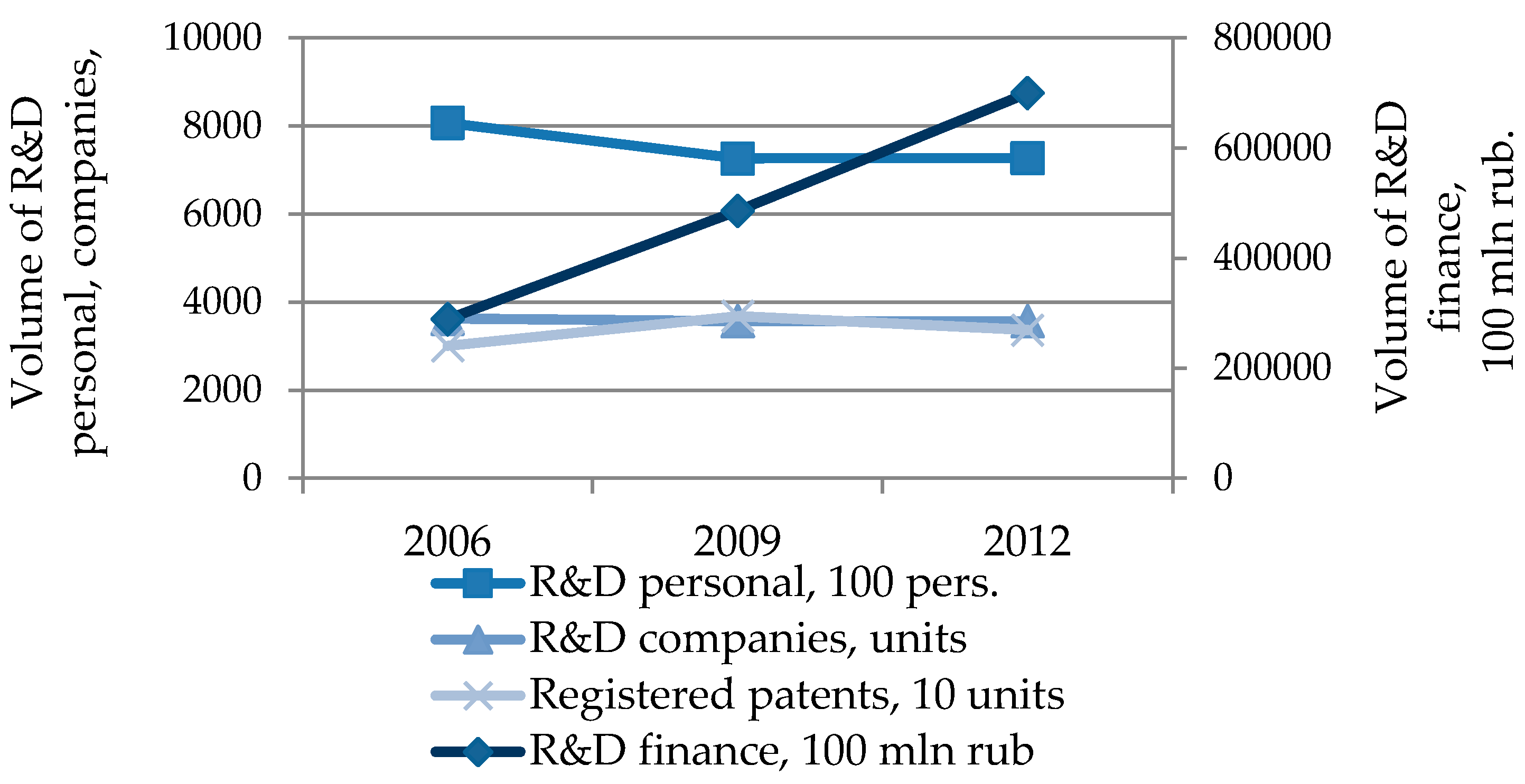
The level of innovative development in the Russian Federation varies across regions depending on the level of productive forces development, natural and geographical conditions, historical and socio-economic development, and the territorial distribution of industry and science, so there is a high differentiation and polarization of their number across Russian regions that was reflected in the regional specifics of innovative enterprises financing. These factors inhibit the spillover of innovation capital and innovative evolution.

Initially, the effectiveness of regional innovation systems was evaluated based on the data of 80 regions, as a number of Russian regions in 2006–2017 did not have comparable indicators. However, there was a big gap between the leading regions and regions in which the utilized innovative resources have not led to significant innovative structural shifts in economic development at the macroeconomic level, so the specifics of the territorial and federal structure of the Russian Federation explains the use of cluster analysis for the regions selection.

In the examined set of areas, there were regions that were in better socio-economic conditions and there was a high inter-regional differentiation (relative to other regions) by indicators of territory and economy, which is why spatial indicators characterizing innovative development (volume of innovative goods, domestic R & D costs, patents, and number of innovative companies) varied significantly across Russian regions.

Thus, some regions in terms of innovative development were not of research interest, since the importance of innovative development and, accordingly, their indicators were not significant for economic regional development. They were excluded from examination.

Bringing the original set to a homogeneous form was a separate data mining task. Within the framework of the study, it was necessary to carry out stratification of regions so that we could single out homogeneous groups and select comparable objects; therefore, we conducted a cluster analysis according to the indicators chosen for analysis: high-tech share in GRP, investment share in fixed assets, volume of innovation goods, and internal R & D costs.

As a result of cluster analysis, regions were divided by several essential features. In addition, the cluster analysis allowed us to reduce large amounts of socio-economic information and to make them compact and homogeneous. These features seemed essential for the preliminary processing of regional development data in combination with DEA methods.

Clustering consists of dividing an analyzed set into groups of similar objects that are called clusters. The task of the clustering algorithm is the distribution of objects among clusters, the separation of large and the organization of small clusters, and then the redistribution of objects between them [34,35].

There are a various clustering techniques for unsupervised learning such as:

• Partitional (k-means, k-medoids, k-mode, Clustering LARge Applications (CLARA) and Clustering Large Applications based on RAN-Domized Search (CLARANS).
• Hierarchical (agglomerative and divisive).
• Density-based spatial clustering of applications with noise.
• Distribution-based statistical clustering model (expectation-maximization clustering).
• Fuzzy analysis clustering (c-means).
• Self-organizing maps.

The most commonly used clustering algorithms are non-hierarchical, such as the k-means and k-medoids algorithms.

k-medoids is a greedy algorithm; it is a modification of k-means that does not use linear space properties and that uses compactness as criteria of clustering [36]. A medoid is the point in the cluster with minimal average dissimilarities to the other data points.

A significant advantage in this regional study was that the k-medoid algorithm is less sensitive to outliers than other partitional algorithms—k-means, in particular.

The common realization of k-medoid is an iterative algorithm (partitioning around medoid) that minimizes the sum of distances from each object to its cluster medoid. Its metrics is as follows:

• Input: dataset A of L data points, number of clusters k.
• Output: partition the data points from A into k clusters $\mathrm{C}=\left\{{\mathrm{C}}_1,{\mathrm{C}}_2,\dots ,{\mathrm{C}}_{\mathrm{k}}\right\}$.
• Initialization: randomly select the k of the L data points for the medoids set M.
• Build-step: determine the closest medoid m for each point a∈A.
• Swap-step: for each medoid m∈M and each data point a associated to m, swap m and a and calculate the value of the intercluster distance d as the average dissimilarity of a to all the data points associated to m. Select the medoid a with the minimum cost of the configuration distance d.
• Repeat steps 2 and 3 until the medoids do not change or other termination criteria are met.

In order to use a clustering algorithm and implement separation, it is required to choose a similarity measure. The measure of similarity is a function that determines the distance between objects in multidimensional space. The similarity measure is selected based on attribute types, as well as computational complexity requirements. The distance metrics are classified as follows:

• Mixed measures (mixed Euclidean distance).
• Nominal measures (Nominal distance, Dice similarity, Jaccard similarity, Kulczynski similarity, Rogers Tanimoto similarity, Russell Rao similarity, and simple matching similarity).
• Numerical measures (Euclidean distance, Camberra distance, Chebychev distance, correlation similarity, cosine similarity, Dice similarity, and Jaccard similarity).
• Bregman divergences (generalized divergence, Itakura–Saito distance, Kullback–Leibler divergence, and Mahalanobis distance).

The approach based on Bregman divergences are the generalized distance measures [37]. There exists a corresponding generalized distance measure (squared Euclidean distance, Kullback–Leibler distance, Itakura–Saito distance, and others) for the probability distribution family. It should be noted that some types of divergence provide better cluster separability.

The Bregman divergence represents a convex on a convex set:

$$d_{\phi }\left(x,y\right)=\phi \left(x\right)-\phi \left(y\right)-\nabla \phi \left(y\right) \left(x-y\right).$$

(1)

where $\phi \left(x\right)$ is a strictly convex, continuously-differentiable function on a convex set, and ∇φ(y) is its derivative on y. Bregman divergences are not a metric. In a generalized divergence case, the convex function in r-dimensional real vector space is:

$$\phi \left(x\right)={{\displaystyle \sum }}_{j=1}^r{x}_{j}log{x}_j,$$

(2)

$$d_{\phi }\left(x,y\right)={{\displaystyle \sum }}_{j=1}^r{x}_{j}log\left(\frac{x_j}{y_j}\right)-{{\displaystyle \sum }}_{j=1}^r(x_j-y_j).$$

(3)

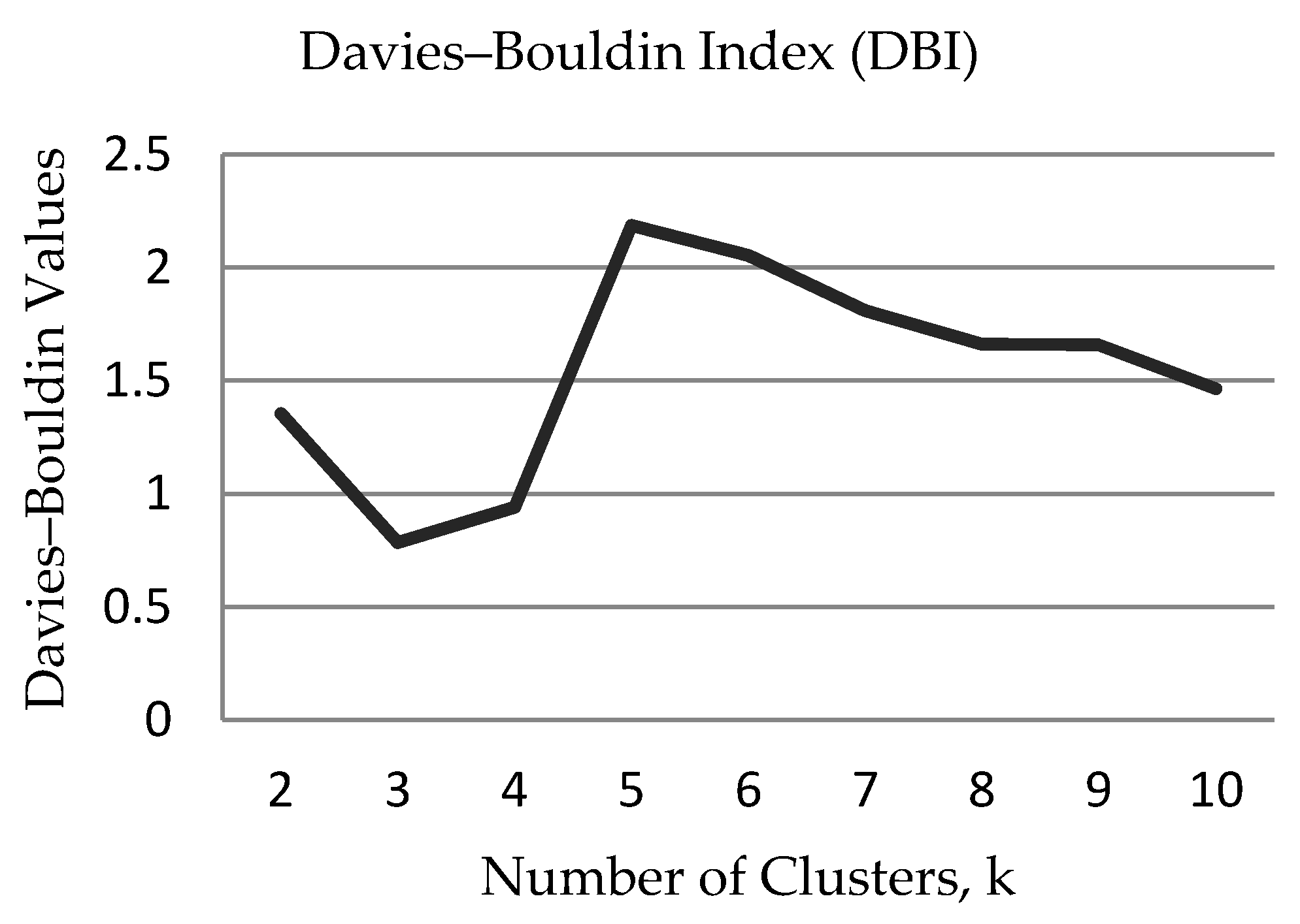
Many indicators used to measure clustering accuracy (Rand, Jaccard Index, F-measure, mutual information, and Fowlkes–Mallows) are external validation methods that require target variables. Indices like those of Davies–Bouldin, Dunn, and Silhouette can be used as internal metrics for evaluating clustering algorithms.

A significant drawback of non-hierarchical methods is the need to specify the number of clusters k. The Davies–Bouldin score is used to evaluate the optimal number of clusters [38].

Let $S_i=\frac{1}{\left|C_i\right|}{\displaystyle \sum }_{a\in C_i}d\left(a,m_i\right)$ be the intra-cluster distance of $C_i$. $d_{ij}=d\left(C_i,C_j\right)$ is the inter-cluster distance between $C_i$ and $C_j$.

Here is an option for calculating similarity, determined by the formula:

$$R_{ij}=\frac{S_i+S_j}{d_{ij}}.$$

(4)

The Davies–Bouldin Index (DBI) is calculated as follows:

$$DBI\left(C\right)=\frac{1}{k}{\displaystyle \sum }_{i=1}^k{R}_i ,$$

(5)

where $R_i=ma{x}_{i,j\in \left\{1\dots k\right\},i\ne j}\left(R_{ij}\right),i=1,\dots ,k$.

A low DBI value indicates a more appropriate cluster structure.

Data preparation is an important part of cluster analysis. As the normalization method, we used proportion transformation. As a result of such normalization, each value was divided by the total sum of that attribute values ignoring non-numeric or missing values. In this case, the normalized attribute values were positive in accordance with the necessary requirements of the used DEA method.

3.2. DEA Malmquist Index Modeling

The methodology for assessing the dynamics of region innovative development and innovative spillovers was based on the application of the DEA model with the Malmquist Productivity Index. DEA is a linear programming methodology that uses input and output data for a group of homogeneous objects in order to build a piece-wise linear production frontier for each object in the sample. The DEA provides an estimation of the efficiency relative to the best practices under the condition that the technology is fixed at current level. To construct the frontier, linear programming problems are solved (for each object in the sample, a separate problem is formulated and solved). The degree of technical inefficiency of each object is defined as the distance between the observed data point and the frontier. DEA makes it possible to obtain a quantitative evaluation of the analyzable entities that are usually called decision-making units (DMU).

Currently there are different types of DEA models depending on orientation (input-oriented and output-oriented), returns to scale (constant return to scale (CRS) and variable returns to scale (VRS)), distance function, frontier type, and other aspects [39]. In an input-oriented model, the DEA method constructs the frontier by searching for the maximum possible proportional reduction of input data with constant output levels for each object. In the output-oriented model, the DEA method defines the maximum proportional increase in production output under assumption fixed input levels. These two approaches give the same estimations of technical efficiency when applying the CRS model, but they are unequal in the VRS model.

The Malmquist Index is used to evaluate technological efficiency obtained for relatively different sets of objects [40,41,42]. The Malmquist Index measures the total factor productivity change of a DMU between two consecutive time periods. It is defined as the product of a change in efficiency (catch-up) and technological change (shift of the border). A change in efficiency reflects the extent to which the DMU improves or deteriorates its effectiveness, while technological changes reflect a change in the frontiers of efficiency between two periods [43].

The total factor productivity (TFP), when using the Malmquist Index methods, changes between two data points (e.g., those of a particular region in two adjacent time periods) by calculating the ratio of the distances of each data point relative to a common technology. The Malmquist TFP change index in output-orientated DEA model between period t and period (t + 1) is:

$$M_o\left(y_{t+1}, x_{t+1},y_t,x_t\right)={\left(\frac{d_o^t\left(x_{t+1}, y_{t+1}\right)}{d_o^t\left(x_t, y_t\right)}·\frac{d_o^{t+1}\left(x_{t+1}, y_{t+1}\right)}{d_o^{t+1}\left(x_t, y_t\right)}\right)}^{0,5},$$

(6)

where $\left(x_{t+1}, y_{t+1}\right)$ and $\left(x_t,y_t\right)$ represent the input and output vector of the period (t + 1) and t, respectively, and the notation $d_o^t\left(x_t,y_t\right)$ represents the distance from the period t to the period (t + 1) technology.

A value of M_o greater than 1 indicates positive TFP growth from period t to period (t + 1). A value of M_o less than 1 indicates a TFP decline. If M_o = 1, there is no progress or regression in period t ratio to (t + 1).

M_o is the geometric mean of two TFP indices. The first is evaluated with respect to period t technology, and the second is evaluated with respect to period (t+1) technology. An equivalent decomposed form of the TFP index [44,45] is:

$$M_o\left(y_{t+1}, x_{t+1},y_t,x_t\right)=\frac{d_o^{t+1}\left(x_{t+1}, y_{t+1}\right)}{d_o^t\left(x_t, y_t\right)}·{\left(\frac{d_o^t\left(x_{t+1}, y_{t+1}\right)}{d_o^{t+1}\left(x_{t+1}, y_{t+1}\right)}·\frac{d_o^t\left(x_t, y_t\right)}{d_o^{t+1}\left(x_t, y_t\right)}\right)}^{0,5}.$$

(7)

Let us consider the first factor in Equation (2), which is named technical efficiency change ($EC)$:

$$EC=\frac{d_o^{t+1}\left(x_{t+1}, y_{t+1}\right)}{d_o^t\left(x_t, y_t\right)}.$$

(8)

$EC$ is the change in the output-oriented measure of technical efficiency between periods t and (t+1), and it shows how the ratio of actual outputs to potential has changed. EC indicates the capability of a DMU to catch up with more efficient DMUs.

The second factor in Equation (2) is technological change ($TEC$):

$$TEC={\left(\frac{d_o^t\left(x_{t+1}, y_{t+1}\right)}{d_o^{t+1}\left(x_{t+1}, y_{t+1}\right)}·\frac{d_o^t\left(x_t, y_t\right)}{d_o^{t+1}\left(x_t, y_t\right)}\right)}^{0,5}.$$

(9)

$TEC$ is the potential index—the geometric mean of two relations—that characterizes the shift of the potential technology frontier between period t6 and (t + 1). In other words, the last relation reflects a change in the technological efficiency of the evaluated object caused by a shift in the effective boundary.

Another process of technical efficiency decomposition is based on using both CRS and VRS DEA frontiers. A scale efficiency change (SEC) can be represented as follows:

$$SEC={\frac{d_{VRS}^t\left(x_{t+1}, y_{t+1}\right)/d_{CRS}^t\left(x_{t+1}, y_{t+1}\right)}{d_{VRS}^t\left(x_t, y_t\right)/d_{CRS}^t\left(x_t, y_t\right)}·\frac{d_{VRS}^{t+1}\left(x_{t+1}, y_{t+1}\right)/d_{CRS}^{t+1}\left(x_{t+1}, y_{t+1}\right)}{d_{VRS}^{t+1}\left(x_t, y_t\right)/d_{CRS}^{t+1}\left(x_t, y_t\right)}}^{0,5}$$

(10)

A pure efficiency change (PEC) is given below:

$$PEC=\frac{d_{VRS}^{t+1}\left(x_{t+1}, y_{t+1}\right)}{d_{CRS}^t\left(x_t, y_t\right)}.$$

(11)

The TFP index can be represented in the form of such factors as the change in efficiency and the technical change. Let for a time period t, t = 1, …, T, DMU_i, i = 1, …, N, use P inputs to produce S outputs. In a particular time period t, the following definitions hold:

• y_i is a S×1 vector of output quantities for the DMU_i.
• x_i is a P×1 vector of input quantities for the DMU_i.
• Y is a N×S matrix of output quantities for all N DMU_i.
• X is a N×P matrix of input quantities for all N DMU_i.
• λ is a N×1 vector of weights.
• $\phi$ is a scalar.

To calculate $M_o\left(y_{t+1},x_{t+1},y_t,x_t\right)$, it is necessary to solve the following linear programming problems [44]:

$$\begin{array}{c}{\left(d_o^t\left(x_t,y_t\right)\right)}^{-1}=ma{x}_{\phi ,\lambda }\phi ,\\ \mathrm{St}\hspace{1em}-\phi y_{i,t}+Y_t \lambda \ge 0,\\ -x_{i,t}+X_t \lambda \ge 0,\\ \lambda \ge 0\end{array}$$

(12)

$$\begin{array}{c}{\left(d_o^{t+1}\left(x_{t+1}, y_{t+1}\right)\right)}^{-1}=ma{x}_{\phi ,\lambda } \phi ,\\ \mathrm{St}\hspace{1em}-\phi y_{i,t+1}+Y_{t+1}\lambda \ge 0,\\ -x_{i,t+1}+X_{t+1}\lambda \ge 0,\\ \lambda \ge 0\end{array}$$

(13)

$$\begin{array}{c}{\left(d_o^t\left(x_{t+1},y_{t+1}\right)\right)}^{-1}=ma{x}_{\phi ,\lambda }\phi ,\\ -\phi y_{i,t+1}+Y_t\lambda \ge 0,\\ -x_{i,t+1}+X_t\lambda \ge 0,\\ \lambda \ge 0\end{array}$$

(14)

$$\begin{array}{c}{\left(d_o^{t+1}\left(x_t,y_t\right)\right)}^{-1}=ma{x}_{\phi ,\lambda }\phi ,\\ -\phi y_{i,t}+Y_{t+1}\lambda \ge 0,\\ -x_{i,t}+X_{t+1}\lambda \ge 0,\\ \lambda \ge 0\end{array}$$

(15)

The above Equations (12)–(15) need to be solved for each DMU in a sample. Hence, the total number of linear programming problems for N DMUs and T time periods is $N·\left(3T-2\right)$.

4. Results

4.1. Clustering of Regions According to the Level of Innovative Development

The specific feature of present study was that in the set of objects under examination, one could observe a situation where resource indicators in terms of the innovation system effectiveness reduce or remain the same, but the performance of the regional innovation systems sharply improves. We tried by means of cluster analysis to take the influence of this phenomenon into account in the evaluation of the innovative development effectiveness and the dynamics assessment for 2006–2017.

The proposed set of indicators allowed for, in principle, the desirable clustering all regions according to integrated assessment of their innovative development rate. To ensure the adequacy of assessment from the sample, it was necessary to exclude regions for which there were no data for the periods under review or where zero values of indicators were observed. The authors applied a cluster analysis to create a balanced data panel.

It was decided to use the following indicators for 2017 to perform cluster analysis:

• High-tech share in GRP, %.
• Investment share in fixed assets, %.
• Volume of innovation goods, rubles.
• Internal R & D costs, million rubles.

For clustering regions, the k-medoids method was applied with Bregman divergence as a distance type. To select the number of clusters k, the Davies–Bouldin Index was used. The Davies–Bouldin criterion was calculated for each number of clusters k = 1, …, 10 (

Table 3. Davies–Bouldin Index for different number of clusters.

k	Davies–Bouldin Index (DBI)
2	1.355
3	0.785
4	0.941
5	2.185
6	2.054
7	1.810
8	1.661
9	1.658
10	1.465

).

The plot (Figure 4) shows that the lowest resulting Davies–Bouldin value occurred at k = 3, thus suggesting that the optimal number of clusters was three.

As a result of applying the cluster model for k = 3, the plot (Figure 3) shows that the lowest resulting Davies–Bouldin value occurred at k = 3, thus suggesting that the optimal number of clusters was three.

There was division of regions into three clusters in accordance with the given model. The description of the of cluster analysis result is presented in

Table 4. The division of the initial 80 constituent entities of the Russian Federation into clusters.

Clusters	Regions
Cluster 0	Arhangelsk Region, Belgorod Region, Vladimir Region, Voronezh Region, St. Petersburg, Kirov Region, Krasnodar Region, Kursk Region, Moscow Region, Nizhny Novgorod Region, Novosibirsk Region, Penza Region, Perm Region, Republic of Bashkortostan, Mari El Republic, Republic of Mordovia, Republic of Tatarstan, Rostov Region, Ryazan Region, Samara Region, Sverdlovsk Region, Stavropol Region, Tomsk Region, Tula Region, Udmurt Republic, Ulyanovsk Region, Khabarovsk Region, Chelyabinsk Region, Chuvash Republic, and Yaroslavl Region
Cluster 1	Altai Region, Altai Republic, Amursk Region, Republic of Buryatia, Astrakhan Region, Republic of Dagestan, Bryansk Region, Republic of Ingushetia, Volgograd Region, Republic of Kalmykia, Vologda Region, Republic of Karelia, Jewish Autonomous Region, Komi Republic, Transbaikal Region, Republic of Sakha (Yakutia), Ivanovo Region, Republic of North Ossetia-Alania, Irkutsk Region, Tyva Republic, Kabardino-Balkarian Republic, Republic of Khakassia, Kaliningrad Region, Saratov Region, Kaluga Region, Sakhalin Region, Kamchatka Region, Smolensk Region, Karachay-Cherkess Republic, Tambov Region, Kemerovo Region, Tver Region, Kostroma Region, Tyumen Region, Krasnoyarsk Region, Chechen Republic, Kurgan Region, and Chukotka Autonomous
Cluster_2	Moscow City

.

Table 5. Cluster centroids for k = 3.

Attribute	Cluster 0	Cluster 1	Cluster 2
Hi-tech share in GRP, %	0.017	0.009	0.014
Investment share in fixed assets, %	0.009	0.010	0.007
Volume of innovation goods, %	0.025	0.003	0.007
Intramural R & D costs, million rubles	0.007	0.000	0.352

shows the characteristics of cluster medoids for the obtained cluster model for the normalized data. In terms of intramural R & D costs, cluster 2 represents an abnormal object. The essential purpose of the preliminary data processing was the selection of abnormal objects. It was necessary to reject outliers that did not fit into the data structure. The results of the preliminary data processing using the cluster analysis allowed us to identify Moscow as an abnormal sample object (cluster 2), which was quite consistent with the expert assessment.

An important step in the visualization of clustering results was the formation of scatter plots and histograms, where the diagonal cells are the distribution plot and others elements correspond to scatter plots for a different pairs of attributes with color coding in accordance to cluster labels (Figure 5). This allowed us to check whether outliers were falling inside cluster influence areas and to detect which clusters were distant to one another. There was no significant correlation between attributes.

A visualization of the cluster analysis results demonstrates the obtained data structure (Figure 6). A bar plot indicates a difference between the cluster’s mean in such normalized model variables as hi-tech share in GRP, investment share in fixed assets, and intramural R & D costs.

As a result of preliminary data analysis by cluster analysis methods, it was proposed to use only a part of the regions for a comparative assessment of technical efficiency. The regions belonging to cluster 0 and cluster 2 are economic objects that are more developed in terms of innovative potential. The regions forming cluster 1 with regard to selected indicators are much less successful in terms of innovative development. It should be noted that in most cluster 1 regions, the indicators that were proposed to be used in DEA models were close to the minimum values. Thus, to assess the innovative development dynamics in these regions, it was further proposed to use 31 regions belonging to clusters 0 and 2.

As a result, 31 out of 80 regions were selected for subsequent analysis; a number of regions were excluded from the analysis due to incomparably polarized indicators or a lack of statistical data. Finally, this allowed us to distinguish two groups of regions—underdeveloped regions and leading regions—in accordance with the level of their innovative development.

4.2. Analysis of Malmquist Productivity Index

To test the research hypotheses, the Malmquist Productivity Index and its components were calculated to assess the dynamics of innovative development over three adjustment periods. Values $M_o>1$ for assessing direct and indirect effects of innovation indicated an increased efficiency of the regions under consideration during the study period. The construction of the Malmquist Index allowed us to obtain an estimate of the region distance from production possibility frontier (EC) characterizing the dynamics of total factor productivity, as well as to reveal the dynamics of technological progress (TEC). The EC indicator made it possible to separate the innovative development dynamics of the region from the change with time of the frontier itself. A TEC value of more than 1 indicated technological progress; otherwise, there was technological degradation in the region development. An analysis of the Malmquist Productivity Index and decomposition results from data of 31 regions of the Russian Federation allowed us to present the tendency of regional innovation system development.

Table 6. Malmquist Productivity Index ($M_o$ ) decomposition for model 1. EC: efficiency change; TEC: technological change; SEC: scale efficiency change; and PEC: pure efficiency change.

Region	EC	TEC	PEC	SEC	${\mathit{M}}_{\mathit{o}}$
Arhangelsk Region	3.479	1.463	1.245	2.794	5.088
Krasnodar Region	2.098	1.973	1.000	2.098	4.138
Kursk Region	1.747	1.374	0.995	1.755	2.400
Khabarovsk Region	1.722	1.337	0.928	1.856	2.302
Mari El Republic	1.167	1.854	1.000	1.167	2.163
Voronezh Region	1.027	1.969	1.503	0.684	2.022
Sverdlovsk Region	1.046	1.834	1.143	0.914	1.918
Tomsk Region	0.899	2.116	0.966	0.930	1.902
Moscow Region	0.691	2.495	0.693	0.997	1.724
Yaroslavskaya Region	1.025	1.644	1.096	0.935	1.685
Republic of Bashkortostan	1.402	1.103	1.502	0.934	1.547
Rostov Region	0.762	2.011	0.805	0.947	1.534
Udmurt Republic	1.189	1.177	0.861	1.382	1.400
Perm Region	1.000	1.369	1.000	1.000	1.369
Vladimir Region	1.099	1.243	1.328	0.827	1.366
Nizhny Novgorod Region	0.585	2.234	0.510	1.147	1.307
Republic of Mordovia	1.000	1.270	1.000	1.000	1.270
Chelyabinsk Region	0.827	1.404	0.778	1.063	1.161
Chuvash Republic	1.181	0.954	0.938	1.259	1.127
St. Petersburg	0.828	1.335	1.011	0.818	1.105
Tula Region	0.665	1.654	0.733	0.907	1.099
Samara Region	0.549	1.976	0.534	1.029	1.085
Republic of Tatarstan	0.618	1.610	0.615	1.005	0.996
Ryazan Region	0.848	1.156	0.806	1.053	0.980
Belgorod Region	0.561	1.664	0.762	0.736	0.934
Novosibirsk Region	0.740	1.232	0.863	0.857	0.912
Kirov Region	0.871	0.910	1.000	0.871	0.793
Moscow City	2.223	0.336	2.081	1.068	0.748
Stavropol Region	0.978	0.735	1.116	0.876	0.719
Penza Region	0.868	0.653	1.000	0.868	0.567
Ulyanovsk Region	0.553	0.963	0.593	0.932	0.533

and

Table 7. Malmquist Index summary of means for the model 1.

Period	EC	TEC	PEC	SEC	${\mathit{M}}_{\mathit{o}}$
2011–2014	0.597	2.407	0.653	0.914	1.436
2014–2017	1.657	0.763	1.344	1.233	1.263
Mean	0.994	1.355	0.937	1.061	1.347

contain regions with Malmquist Index for a single output (volume of innovation goods) as direct effects of innovation activity.

As for the results of modeling the direct effects of innovative development, regions with $M_o>1$ showed a progress in the period from 2011 to 2017. Other regions (Republic of Tatarstan, Ryazan Region, Belgorod Region, Novosibirsk Region, Kirov Region, Moscow City, Stavropol Region, Penza Region, and Ulyanovsk Region) with $M_o<1$ showed regression in the two periods.

Table 8. Malmquist Index decomposition for the model 2.

Region	EC	TEC	PEC	SEC	${\mathit{M}}_{\mathit{o}}$
Arhangelsk Region	1.000	2.242	1.000	1.000	2.242
Rostov Region	0.649	3.265	1.640	0.396	2.120
Tula Region	1.074	1.941	1.000	1.074	2.085
Udmurt Republic	0.909	2.180	1.000	0.909	1.983
Belgorod Region	1.392	1.354	1.178	1.181	1.884
Kursk Region	0.775	2.364	0.780	0.994	1.831
Samara Region	0.639	2.686	1.578	0.405	1.716
Republic of Mordovia	1.000	1.683	1.000	1.000	1.683
Sverdlovsk Region	1.329	1.239	1.329	1.001	1.647
Mari El Republic	1.000	1.506	1.000	1.000	1.506
Stavropol Region	0.678	2.178	1.000	0.678	1.476
Moscow Region	1.335	1.042	0.750	1.781	1.391
Ryazan Region	0.833	1.585	0.778	1.070	1.320
Republic of Bashkortostan	0.494	2.458	1.062	0.465	1.215
Chuvash Republic	0.718	1.630	1.000	0.718	1.170
Chelyabinsk Region	0.590	1.876	0.885	0.667	1.107
Moscow City	1.283	0.862	1.253	1.024	1.106
Ulyanovsk Region	0.536	2.045	1.000	0.536	1.096
Nizhny Novgorod Region	1.290	0.843	1.000	1.290	1.087
Kirov Region	0.681	1.573	1.000	0.681	1.071
Krasnodar Region	0.493	2.163	0.636	0.775	1.067
Voronezh Region	0.569	1.846	1.222	0.466	1.051
Vladimir Region	0.590	1.642	0.612	0.964	0.968
Republic of Tatarstan	1.000	0.962	1.000	1.000	0.962
Perm Region	1.000	0.923	1.000	1.000	0.923
Khabarovsk Region	0.580	1.310	0.650	0.891	0.760
Penza Region	0.531	1.427	0.566	0.939	0.758
St. Petersburg	0.742	1.014	1.000	0.742	0.753
Novosibirsk Region	0.351	2.044	0.736	0.477	0.717
Tomsk Region	0.331	1.708	0.364	0.909	0.566
Yaroslavskaya Region	0.355	1.003	0.447	0.794	0.356

and

Table 9. Malmquist Index summary of means for the model 2.

Period	EC	TEC	PEC	SEC	${\mathit{M}}_{\mathit{o}}$
2011–2014	1.098	0.888	0.992	1.107	0.975
2014–2017	0.498	2.876	0.826	0.603	1.432
Mean	0.739	1.598	0.905	0.817	1.182

show the Malmquist Index for the model 2 with 3 outputs (hi-tech share in GRP, investment share in fixed assets, and used patents) as indirect effects of innovation activity for the regions.

Regarding the innovative development modeling of the indirect effects results, it should be noted that 71% among the sample of the leading regions with $M_o>1$ demonstrated a progress in period from 2011 to 2017. The remaining regions with $M_o<1$ (Vladimir Region, Republic of Tatarstan, Perm Region, Khabarovsk Region, Penza Region, St. Petersburg, Novosibirsk Region, Tomsk Region, and Yaroslavl Region) showed regression during the two periods.

The assessment results in model 1 on the direct effects of innovation showed that the average dynamics of innovative development was 1.347, and the development dynamics from 2011 to 2014 was lower than from 2014 to 2017. In the post-crisis period from 2014 to 2017, the development dynamics was higher. The average development dynamics of indirect spillover effects in model 2 was 1.182, i.e., there was no positive dynamics in 2011–2014, but growth trends appeared from 2014 to 2017. This demonstrated the nature of the innovative spillover effects manifestation and indicated a higher average growth rate of the direct outcomes of innovation and the ‘delayed’ impact of indirect spillover effects on innovative growth. Figure 7 shows the results of the calculation of the Malmquist Index and its individual components for model 1 and model 2, which corresponded to the assessment of the innovative development dynamics in the regions.

Among well-developed regions, 54.84% had $M_o>1$ in accordance with both models for assessing direct and indirect effects, i.e., there was a steadily innovative development of more than half of the territorial entities from the research sample for the period from 2011 to 2017.

The decomposition into two components additionally demonstrated that the part of the improvement was attained through the technical change rather than through the efficiency change of the relatively inefficient regions catching up with efficient ones. If EC > 1, the technical efficiency reduced the difference with the optimal region. If EC < 1, the technical efficiency increased the difference with the optimal region. The average technical efficiency change index was 0.739, which was less than 1. This objectively indicated that the gap between the levels of innovative system development had significantly increased by the regions during the selected time period.

The technological change index TEC denotes the degree of technical advancement or technical innovation. If TEC > 1, technical advancement was indicated, and TEC < 1 meant that the technology possessed a recessionary tendency. As seen from index decomposing, the average of the technological change index was 1.598, which was greater than 1. This indicated that the technical efficiency indicators of the reference regions increased monotonously.

PEC and SEC can be used to identify main direction of further catching up the frontier in region innovation system. In model 1 for the direct effects of innovation process, PEC = 0.937, which reflected the decreasing impact of technical and management factors. SEC = 1.061 for model 1 indicated the main influence on regional innovation system by scale factors. As for model 2 with indirect factors of innovation process, PEC = 0.905 and SEC = 0.817, thus indicating an insufficient use of both technical and management capabilities and scale economy factors. It should be noted that for model 2 with indirect innovation factors, the value of SEC as less than for model 1. Since SEC mainly depends on institutional arrangement, we can conclude that there was a negative spillover trend.

Figure 8 shows the average values of the decomposed Malmquist Index for two models related to the assessment of the direct and indirect effects of innovation.

The component of the Malmquist Index $EC<1$ as a relative change in the technical efficiency of individual regions between periods characterized the possibilities of catching up development and showed an increased technological gap of the bulk of the regions from the leaders. The efficiency frontier shift or technology change $TEC>1$ characterized the opportunities for the advanced development of leaders and reflected technology improvement.

The significance of obtained results is as follows. A decrease in technical efficiency in unfavorable environment conditions was established, whereas there was a shift of the regional efficient frontier. A change in the index components (efficiency shift and technology change) suggested that in an unfavorable environment, the technological frontier is moving and there has been no catch-up development among the regions.

5. Discussion

The results of the plant-level data analysis over the period 2011–2017 indicated the growth of total factor productivity of regional innovation development on average. At the same time, 2014–2017 observed a negative trend in the dynamics of the direct effects of innovative development. The evaluation of innovation activity effectiveness in terms of indirect effects demonstrated positive dynamics in Russia (H1). This may indicate the impact of innovation policy on the innovative development in the regions.

The average value of technical efficiency change for both models with direct and indirect effects was less than 1. This demonstrated a reduction in changes reflecting the diffusion effects of technology. Moreover, when the direct effects model showed positive dynamics in 2014–2017, then the spillover effects showed a negative trend in the past period. This indicated a growing gap between the levels of region innovation development (H2), which in its turn revealed the process of polarization in regional innovative development and its decreased effectiveness.

The reverse trend was observed for technological change recording shifts in the frontier. In the period of 2014–2017, the value of the regions’ technological changes indicated a downward trend in respect to direct effects of region innovation development. We could see significant growth in the indirect effect in 2014–2017.

The change in the effectiveness scale on average for all time periods indicated a downward trend according to the direct effects model and the upwards trend for the indirect effects mode. This indicated that the main source of innovative development is mostly the economy of scale (H3). This gives evidence of an extensive resource type of economic growth, where the effectiveness of regional innovation systems grows only due to the expansion of resources rather than due to their effective use.

Compared with previous studies, we proposed a methodology for assessing the innovation results in terms of direct and indirect effects of innovation in order to estimate what factors are responsible for the innovative development of a region—by expanding resources or by using them effectively. Russian regions were ranked according to changes in their total factor productivity and the dynamics rate of regional innovative development; we identified leaders and outsiders in terms of direct and indirect effects of innovation. Our study made it possible to identify promising regions in terms of innovation growth and revealed the reasons for this effectiveness.

Previous results and literature findings [17,21] have established that over the past few years, the effectiveness of Russian regional innovation systems has increased, and the most efficient innovation development has resulted in the largest agglomerations and technologically developed regions with leading universities and research centers. We also confirmed the findings about the positive dynamics of innovative development in Russia for 2010–2017; however, at the same time, the polarization of regions has been increasing, while the effectiveness of innovative development has been decreasing. Our study showed that the regions that have been witnessing significant growth over our chosen 15 year period do not belong to research and university centers, and the growth of their innovation indicators is caused not by patent activity but by some other factors.

Previous Russian studies have employed the results of patenting as their resulting parameters. We expanded the set of output parameters, which is relevant for the Russian specifics of “not exactly accurate” patent statistics. Many Russian regions fail to demonstrate high patent activity, but at the same time, they have good indicators of the innovation development rate. We differentiated the direct and indirect effects of the innovation process and tried to draw attention to the complexity and multifactorial nature of evaluating innovative system effectiveness. Thus, the growth of the resulting factors for innovative development was extensive and occurred due to resource factors.

Our study was designed to draw attention to the fact that the standard statistical approach for assessing the effectiveness of innovative development needs to be expanded. The DEA Malmquist Index and cluster analysis that we used made it possible to consider the inconsistency in the development of Russian innovation systems due to the vast territory and extreme heterogeneity of the economic development in the Russian regions. Our approach and the proposed models allowed us to obtain significant conclusions and identify those regions that, with a decrease in resourcing, have demonstrated an increase in the resulting indicators. What regions are more efficient and what are the reasons for getting better results of innovation should be known. This is important for the process of making innovative decisions and influencing regional politics, and this is particularly important for the identification of regions with best practices. Realizing this information will enable the drawing of attention to the best practices of these regions and the conducting of benchmarking with other ones.

This finding could be important in terms of policy realization. The results can be used to diagnose effectiveness and prioritize regional innovation policies for specific regions, as well as to justify public investments in R & D, the development of mechanisms for attracting investors’ funds in innovations, the improvement of legislative documents regulating innovative activity, and the development of measures to promote the innovation sphere to solve the problems of innovative development of the Russian economy.

6. Conclusions

The paper presents a study of innovation system effectiveness in Russian regions based on cluster analysis and a DEA Malmquist Index. As a result, conclusions were drawn about the movement of the technology frontier shift and the dynamics of regional innovation development in Russian regions.

To assess direct and indirect innovation effects, the study used indicators for the dynamics of changes in the growth rate of regional innovative development in Russian regions for two periods: 2011–2014 and 2014–2017. The analysis was carried out according to the following variables: the volume of innovative products and the increase in innovative activity, the increase in the share of high-tech products in the GRP structure, the number of patents introduced as a result of intellectual property use, and the growth of financial and investment activity in the economy.

There were some limitations to the present analysis that could form interesting topics for further research. The peculiarity of current investigation was that the sensitivity analysis of dynamic Malmquist DEA models was complicated by the limited availability of statistical data for long periods and the insufficiency of economic performance to explain the nature and specialty of the regional innovative dynamics.

An assessment of innovation development could reveal other aspects in the analysis of regional strategy. Further research should be aimed at identifying the root causes of the innovative effectiveness growth in these regions. A respective analysis of the particular regions would be an extension of great interest. It would be useful to apply additional DEA methods and stochastic frontier analysis models that would allow us to compare models and supplement sensitivity analysis based on econometric approaches. A logical continuation of the research would be the extension of the time interval.

References

1. Grillitsch, M.; Nilsson, M. Innovation in peripheral regions: Do collaborations compensate for a lack of local knowledge spillovers? Ann. Reg. Sci. 2015, 54, 299–321. [Google Scholar] [CrossRef] [Green Version]
2. Audretsch, D.B.; Belitski, M. The role of R&D and knowledge spillovers in innovation and productivity. Eur. Econ. Rev. 2020, 123, 103391. [Google Scholar]
3. Feldman, M. The Geography of Innovation; Kluwer Academic Publishers: Boston, MA, USA, 1994. [Google Scholar]
4. Boschma, R.A. Proximity and innovation: A critical assessment. Reg. Stud. 2005, 39, 61–74. [Google Scholar] [CrossRef]
5. Firsova, A.A.; Makarova, E.L.; Tugusheva, R.R. Institutional Management Elaboration through Cognitive Modeling of the Balanced Sustainable Development of Regional Innovation Systems. J. Open Innov. Technol. Mark. Complex. 2020, 6, 32. [Google Scholar] [CrossRef]
6. Farrell, M.J.; Fieldhouse, M. Estimating efficient production functions under increasing returns to scale. J. R. Stat. Soc. Ser. A 1962, 125, 252–267. [Google Scholar] [CrossRef]
7. Charnes, A.; Cooper, W.W.; Rhodes, E. Measuring the efficiency of decision making units. Eur. J. Oper. Res. 1978, 2, 429–444. [Google Scholar] [CrossRef]
8. Foddi, M.; Usai, S. Regional Knowledge Performance in Europe. Growth Chang. 2013, 44, 258–286. [Google Scholar] [CrossRef]
9. Zabala-Iturriagagoitia, J.M.; Jiménez-Sáez, F.; Castro-Martínez, E.; Gutierrezgracia, A. What indicators do (or do not) tell us about Regional Innovation Systems. Scientometrics 2007, 70, 85–106. [Google Scholar] [CrossRef]
10. Matei, M.M.; Aldea, A. Ranking National Innovation Systems According to their technical Efficiency. Procedia Soc. Behav. Sci. 2012, 62, 968–974. [Google Scholar] [CrossRef] [Green Version]
11. Stejskal, J.; Nekolová, K.; Rouag, A. The use of the weighted sum method to determine the level of development in regional innovation systems—Using Czech regions as examples. Ekon. Časopis Časopis Ekon. Teóriu Hospodársku Polit. Spoločensko-Ekon. Prognózovanie 2015, 63, 239–258. [Google Scholar]
12. Chen, K.; Guan, J. Measuring the efficiency of China’s regional innovation systems: Application of network data envelopment analysis (DEA). Reg. Stud. 2012, 46, 355–377. [Google Scholar] [CrossRef]
13. Chen, K.; Kou, M. Staged efficiency and its determinants of regional innovation systems: A two-step analytical procedure. Ann. Reg. Sci. 2014, 52, 627–657. [Google Scholar]
14. Elias, G.; Goletsis, Y.; Grigoroudis, E. Multi-level multi-stage efficiency measurement: The case of innovation systems. Oper. Res. 2015, 15, 253–274. [Google Scholar]
15. Xuanli, L. A KPCA and DEA Model for Region Innovation Efficiency; Shen, G., Huang, X., Eds.; ECWAC, Part I; Communications in Computer and Information Science, Springer: Berlin/HeIdelberg, Germany, 2011; pp. 109–114. [Google Scholar]
16. Broekel, T.; Rogge, N.; Brenner, T. The innovation efficiency of German regions—A shared-input DEA approach. Rev. Reg. Res. 2018, 38, 77–109. [Google Scholar] [CrossRef] [Green Version]
17. Baburin, V.L.; Zemtsov, S.P. How to assess an efficiency of regional innovation systems in Russia? Innovation 2017, 2, 60–66. [Google Scholar]
18. Zemtsov, S.P.; Kotsemir, M.N. An Assessment of Regional Innovation System Efficiency in Russia: The Application of the DEA Approach. Scientometrics 2019, 120, 375–404. [Google Scholar] [CrossRef]
19. Firsova, A.; Chernyshova, G. Analysis of efficiency of regional innovation systems taking into account the financing structure. In Proceedings of the International Scientific Conference “Competitive, Sustainable and Secure Development of the Regional Economy: Response to Global Challenges” (CSSDRE 2018), Volgograd, Russia, 18–20 April 2018; pp. 417–422. [Google Scholar]
20. Didenko, A.; Loseva, O.V.; Abdikeev, N. Measuring Efficiency of Regional Innovation System with DEA and PCA. In Proceedings of the 2017 IEEE 11th International Conference on Application of Information and Communication Technologies (AICT), Moscow, Russia, 20–22 September 2017; pp. 1–4. [Google Scholar]
21. Rudskaya, I.; Rodionov, D. Econometric modeling as a tool for evaluating the performance of regional innovation systems (with regions of the Russian Federation as the example). Acad. Strateg. Manag. J. 2017, 16, S2. [Google Scholar]
22. Oslo Manual: Guidelines for Collecting and Interpreting Innovation Data, 4th ed.; Manual, OECD, Eurostat: Paris, France, 2018.
23. Frascati Manual: Guidelines for Collecting and Reporting Data on Research and Experimental Development, The Measurement of Scientific, Technological and Innovation Activities; OECD Publishing: Paris, France, 2015.
24. The Measurement of Scientific, Technological and Innovation Activities; OECD Library: Paris, France, 2015; Available online: http://www.oecd-ilibrary.org/science-and-technology/the-measurement-of-scientific-technological-and-innovation-activities_24132764 (accessed on 7 July 2017).
25. Feodorova, E.A.; Korkmazova, B.K.; Muratov, M.A. Spillover effects in the Russian economy: Regional specifics. Reg. Econ. 2016, 1, 139–149. [Google Scholar] [CrossRef]
26. Firsova, A.A.; Narhova, A.A. International Approaches to Assessment of University for Regional Development. Izv. Saratov Univ. Ser. Econ. Manag. Law 2014, 14, 289–294. [Google Scholar]
27. Ogurtsova, E.V.; Tugusheva, R.R.; Firsova, A.A. Innovation spillover effects of information and communications technology in higher education. Perspekt. Nauk. Obraz. Perspect. Sci. Educ. 2019, 42, 409–421. [Google Scholar]
28. Balash, V.A.; Balash, O.S.; Faizliev, A.R.; Chistopolskaya, E.V. Modeling the Spatial Effects of the Impact of Innovation on Regional Economic Growth. In Proceedings of the Fourth Workshop on Computer Modelling in Decision Making (CMDM 2019), Atlantis Highlights in Computer Sciences, Saratov, Russia, 14–15 November 2019; pp. 108–114. [Google Scholar]
29. Firsova, A.; Chernyshova, G. Modeling of Regional High Education Systems’ Efficiency by Data Envelopment Analysis. In Proceedings of the Third Workshop on Computer Modelling in Decision Making (CMDM 2018), Advances in Computer Science Research, Saratov, Russia, 14–17 November 2018; pp. 67–73. [Google Scholar]
30. The Russian Federal Service of State Statistics. Available online: http://www.gks.ru/wps/wcm/connect/rosstat_main/rosstat/en/statistics/science_and_innovations/science (accessed on 25 July 2019).
31. Firsova, A.A.; Chernyshova, G.Y. Mathematical Models for Evaluation of the Higher Education System Functions with DEA Approach. Izv. Saratov Univ. Ser. Math. Mech. Inform. 2019, 19, 351–362. [Google Scholar] [CrossRef]
32. Firsova, A.; Chernyshova, G. Modeling of Regional Innovation Spillover Effects Based on DEA Malmquist Index. In Proceedings of the Fourth Workshop on Computer Modelling in Decision Making (CMDM 2019), Atlantis Highlights in Computer Sciences, Saratov, Russia, 14–15 November 2019; pp. 103–107. [Google Scholar]
33. Aggarwal, C.C. Data Clustering; Chapman and Hall/CRC: Boca Raton, FL, USA, 2013. [Google Scholar]
34. Wierzchoń, S.T.; Kłopotek, M.A. Modern Algorithms of Cluster Analysis; Springer: Berlin, Germany, 2018. [Google Scholar]
35. Kaufman, L.; Rousseeuw, P.J. Clustering by means of medoids. In Statistical Data Analysis Based on the L1-Norm and Related Methods; Dodge, Y., Ed.; Elsevier: North-Holland, Amsterdam, 1987; pp. 405–416. [Google Scholar]
36. Bregman, L.M. The relaxation method of finding the common points of convex sets and its application to the solution of problems in convex programming. USSR Comput. Math. Math. Phys. 1967, 7, 200–217. [Google Scholar] [CrossRef]
37. Davies, D.L.; Bouldin, D.W. A Cluster Separation Measure. IEEE Trans. Pattern Anal. Mach. Intell. 1979, 2, 224–227. [Google Scholar] [CrossRef]
38. Tone, K. Advances in DEA Theory and Applications: With Extensions to Forecasting Models; John Wiley & Sons: Hoboken, NJ, USA, 2017. [Google Scholar]
39. Malmquist, S. Index numbers and indifference surfaces. Trab. Estat. 1953, 4, 209–242. [Google Scholar] [CrossRef]
40. Coelli, T.; Rao, D.S.P.; Battese, G.E. An Introduction to Efficiency and Productivity Analysis, 2nd ed.; Springer: New York, NY, USA, 2005. [Google Scholar]
41. Thanassoulis, E. Introduction to the Theory and Application of Data Envelopment Analysis: A Foundation Text with Integrated Software; Kluwer Academic Publishers: Boston, MA, USA, 2001. [Google Scholar]
42. Caves, D.W.; Christensen, L.R.; Diewert, W.E. The Economic Theory of Index Numbers and the Measurement of Input, Output, and Productivity. Econometrica 1982, 50, 1393–1414. [Google Scholar] [CrossRef]
43. Farrell, M.J. The measurement of productive efficiency. J. R. Stat. Soc. Ser. A 1957, 120, 253–290. [Google Scholar] [CrossRef]
44. Färe, R.; Grosskopf, S.; Primont, D. Aggregation, Efficiency, and Measurement; Springer: New York, NY, USA, 2007. [Google Scholar]
45. Cooper, W.; Seiford, L.; Zhu, J. Data Envelopment Analysis: History, Models, and Interpretations. In International Series in Operations Research & Management Science; Springer: Boston, MA, USA, 2011; pp. 1–39. [Google Scholar]
Figure 1. Variables of innovation activity for 2006–2009–2012.
Information 11 00294 g001
Figure 2. Resulting variables of innovation activity for 2011–2014–2017.
Information 11 00294 g002
Figure 3. Representation of inputs and outputs, taking time lag into account.
Information 11 00294 g003
Figure 4. Cluster number estimation with the Davies–Bouldin Index (DBI).
Information 11 00294 g004
Figure 5. Scatter plot matrix with histogram for region clustering.
Information 11 00294 g005
Figure 6. Standardized medoids for cluster 0 and cluster 1.
Information 11 00294 g006
Figure 7. Malmquist Index for direct (model 1) and indirect (model 2) effects of innovation.
Information 11 00294 g007
Figure 8. Averages of technical change, efficiency change, and Malmquist Index during two periods.
Information 11 00294 g008