3.1. Data Preprocessing by Cluster Analysis
A cluster analysis was used as an initial stage in assessing the dynamics of regional development. To apply the DEA method using the Malmquist Index, it is advisable to distinguish groups of regions that have similar characteristics in terms of innovative development. The uneven development of the regions led to a high differentiation of indicators used in the DEA analysis process and necessitated the alignment of the initial data.
The level of innovative development in the Russian Federation varies across regions depending on the level of productive forces development, natural and geographical conditions, historical and socio-economic development, and the territorial distribution of industry and science, so there is a high differentiation and polarization of their number across Russian regions that was reflected in the regional specifics of innovative enterprises financing. These factors inhibit the spillover of innovation capital and innovative evolution.
Initially, the effectiveness of regional innovation systems was evaluated based on the data of 80 regions, as a number of Russian regions in 2006–2017 did not have comparable indicators. However, there was a big gap between the leading regions and regions in which the utilized innovative resources have not led to significant innovative structural shifts in economic development at the macroeconomic level, so the specifics of the territorial and federal structure of the Russian Federation explains the use of cluster analysis for the regions selection.
In the examined set of areas, there were regions that were in better socio-economic conditions and there was a high inter-regional differentiation (relative to other regions) by indicators of territory and economy, which is why spatial indicators characterizing innovative development (volume of innovative goods, domestic R & D costs, patents, and number of innovative companies) varied significantly across Russian regions.
Thus, some regions in terms of innovative development were not of research interest, since the importance of innovative development and, accordingly, their indicators were not significant for economic regional development. They were excluded from examination.
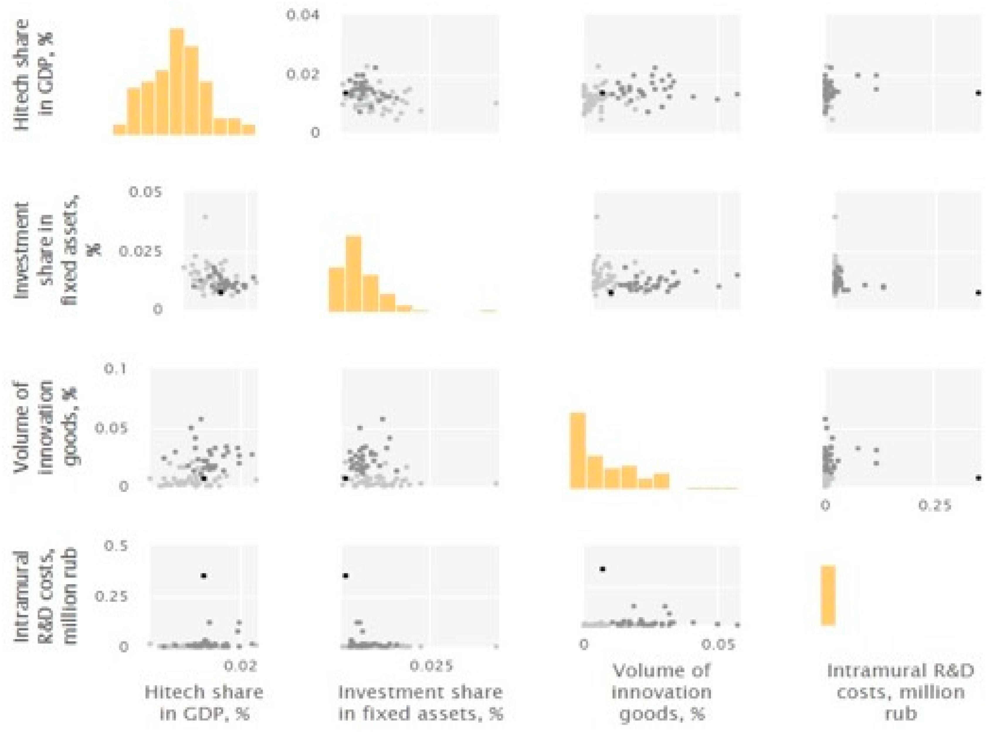
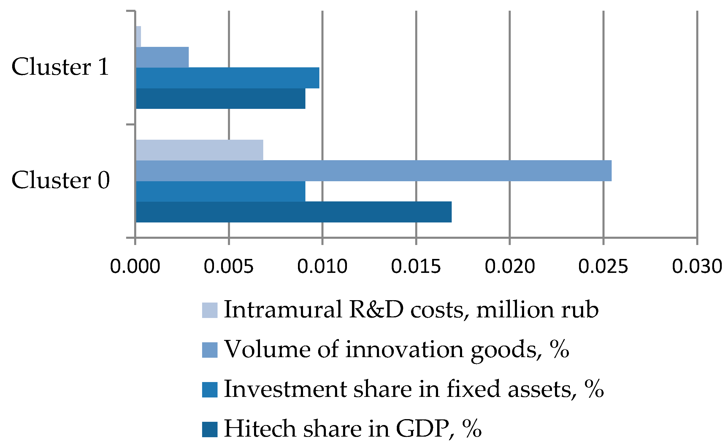
Bringing the original set to a homogeneous form was a separate data mining task. Within the framework of the study, it was necessary to carry out stratification of regions so that we could single out homogeneous groups and select comparable objects; therefore, we conducted a cluster analysis according to the indicators chosen for analysis: high-tech share in GRP, investment share in fixed assets, volume of innovation goods, and internal R & D costs.
As a result of cluster analysis, regions were divided by several essential features. In addition, the cluster analysis allowed us to reduce large amounts of socio-economic information and to make them compact and homogeneous. These features seemed essential for the preliminary processing of regional development data in combination with DEA methods.
Clustering consists of dividing an analyzed set into groups of similar objects that are called clusters. The task of the clustering algorithm is the distribution of objects among clusters, the separation of large and the organization of small clusters, and then the redistribution of objects between them [
34,
35].
There are a various clustering techniques for unsupervised learning such as:
Partitional (k-means, k-medoids, k-mode, Clustering LARge Applications (CLARA) and Clustering Large Applications based on RAN-Domized Search (CLARANS).
Hierarchical (agglomerative and divisive).
Density-based spatial clustering of applications with noise.
Distribution-based statistical clustering model (expectation-maximization clustering).
Fuzzy analysis clustering (c-means).
Self-organizing maps.
The most commonly used clustering algorithms are non-hierarchical, such as the k-means and k-medoids algorithms.
k-medoids is a greedy algorithm; it is a modification of k-means that does not use linear space properties and that uses compactness as criteria of clustering [
36]. A medoid is the point in the cluster with minimal average dissimilarities to the other data points.
A significant advantage in this regional study was that the k-medoid algorithm is less sensitive to outliers than other partitional algorithms—k-means, in particular.
The common realization of k-medoid is an iterative algorithm (partitioning around medoid) that minimizes the sum of distances from each object to its cluster medoid. Its metrics is as follows:
Input: dataset A of L data points, number of clusters k.
Output: partition the data points from A into k clusters .
Initialization: randomly select the k of the L data points for the medoids set M.
Build-step: determine the closest medoid m for each point a∈A.
Swap-step: for each medoid m∈M and each data point a associated to m, swap m and a and calculate the value of the intercluster distance d as the average dissimilarity of a to all the data points associated to m. Select the medoid a with the minimum cost of the configuration distance d.
Repeat steps 2 and 3 until the medoids do not change or other termination criteria are met.
In order to use a clustering algorithm and implement separation, it is required to choose a similarity measure. The measure of similarity is a function that determines the distance between objects in multidimensional space. The similarity measure is selected based on attribute types, as well as computational complexity requirements. The distance metrics are classified as follows:
Mixed measures (mixed Euclidean distance).
Nominal measures (Nominal distance, Dice similarity, Jaccard similarity, Kulczynski similarity, Rogers Tanimoto similarity, Russell Rao similarity, and simple matching similarity).
Numerical measures (Euclidean distance, Camberra distance, Chebychev distance, correlation similarity, cosine similarity, Dice similarity, and Jaccard similarity).
Bregman divergences (generalized divergence, Itakura–Saito distance, Kullback–Leibler divergence, and Mahalanobis distance).
The approach based on Bregman divergences are the generalized distance measures [
37]. There exists a corresponding generalized distance measure (squared Euclidean distance, Kullback–Leibler distance, Itakura–Saito distance, and others) for the probability distribution family. It should be noted that some types of divergence provide better cluster separability.
The Bregman divergence represents a convex on a convex set:
where
is a strictly convex, continuously-differentiable function on a convex set, and ∇
φ(y) is its derivative on y. Bregman divergences are not a metric. In a generalized divergence case, the convex function in r-dimensional real vector space is:
Many indicators used to measure clustering accuracy (Rand, Jaccard Index, F-measure, mutual information, and Fowlkes–Mallows) are external validation methods that require target variables. Indices like those of Davies–Bouldin, Dunn, and Silhouette can be used as internal metrics for evaluating clustering algorithms.
A significant drawback of non-hierarchical methods is the need to specify the number of clusters k. The Davies–Bouldin score is used to evaluate the optimal number of clusters [
38].
Let be the intra-cluster distance of . is the inter-cluster distance between and .
Here is an option for calculating similarity, determined by the formula:
The Davies–Bouldin Index (DBI) is calculated as follows:
where
.
A low DBI value indicates a more appropriate cluster structure.
Data preparation is an important part of cluster analysis. As the normalization method, we used proportion transformation. As a result of such normalization, each value was divided by the total sum of that attribute values ignoring non-numeric or missing values. In this case, the normalized attribute values were positive in accordance with the necessary requirements of the used DEA method.
3.2. DEA Malmquist Index Modeling
The methodology for assessing the dynamics of region innovative development and innovative spillovers was based on the application of the DEA model with the Malmquist Productivity Index. DEA is a linear programming methodology that uses input and output data for a group of homogeneous objects in order to build a piece-wise linear production frontier for each object in the sample. The DEA provides an estimation of the efficiency relative to the best practices under the condition that the technology is fixed at current level. To construct the frontier, linear programming problems are solved (for each object in the sample, a separate problem is formulated and solved). The degree of technical inefficiency of each object is defined as the distance between the observed data point and the frontier. DEA makes it possible to obtain a quantitative evaluation of the analyzable entities that are usually called decision-making units (DMU).
Currently there are different types of DEA models depending on orientation (input-oriented and output-oriented), returns to scale (constant return to scale (CRS) and variable returns to scale (VRS)), distance function, frontier type, and other aspects [
39]. In an input-oriented model, the DEA method constructs the frontier by searching for the maximum possible proportional reduction of input data with constant output levels for each object. In the output-oriented model, the DEA method defines the maximum proportional increase in production output under assumption fixed input levels. These two approaches give the same estimations of technical efficiency when applying the CRS model, but they are unequal in the VRS model.
The Malmquist Index is used to evaluate technological efficiency obtained for relatively different sets of objects [
40,
41,
42]. The Malmquist Index measures the total factor productivity change of a DMU between two consecutive time periods. It is defined as the product of a change in efficiency (catch-up) and technological change (shift of the border). A change in efficiency reflects the extent to which the DMU improves or deteriorates its effectiveness, while technological changes reflect a change in the frontiers of efficiency between two periods [
43].
The total factor productivity (TFP), when using the Malmquist Index methods, changes between two data points (e.g., those of a particular region in two adjacent time periods) by calculating the ratio of the distances of each data point relative to a common technology. The Malmquist TFP change index in output-orientated DEA model between period
t and period (
t + 1) is:
where
and
represent the input and output vector of the period (
t + 1) and
t, respectively, and the notation
represents the distance from the period
t to the period (
t + 1) technology.
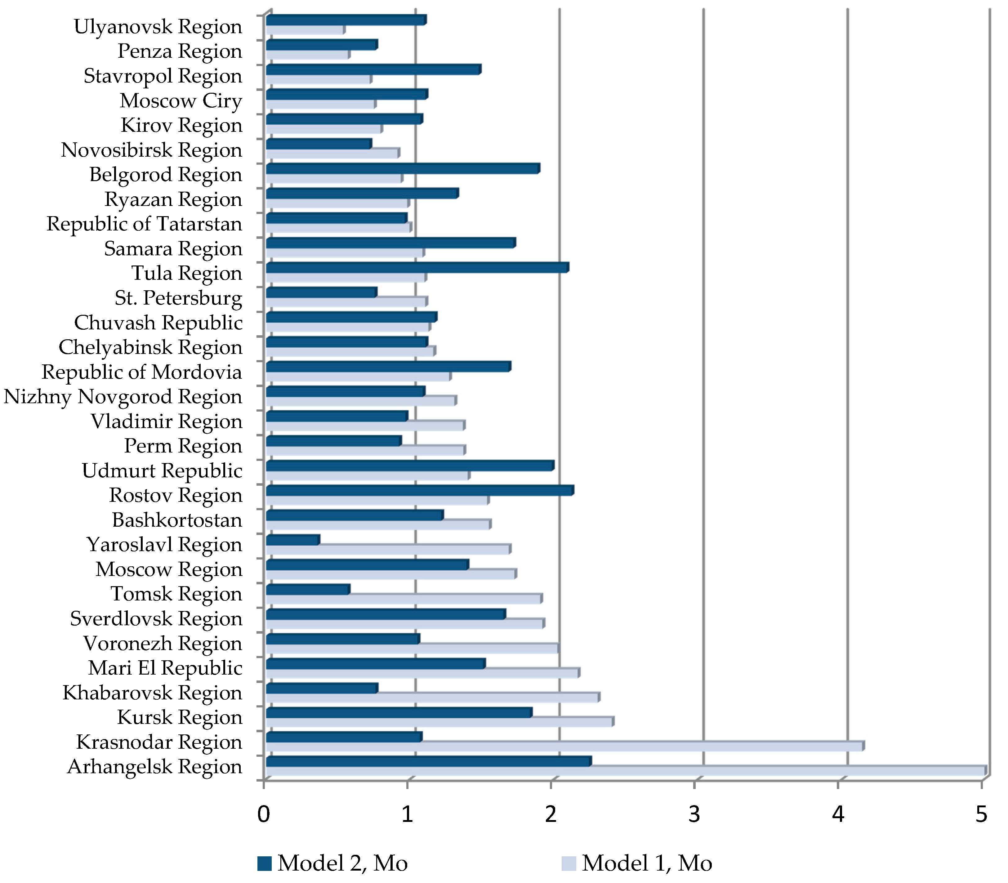
A value of Mo greater than 1 indicates positive TFP growth from period t to period (t + 1). A value of Mo less than 1 indicates a TFP decline. If Mo = 1, there is no progress or regression in period t ratio to (t + 1).
Mo is the geometric mean of two TFP indices. The first is evaluated with respect to period
t technology, and the second is evaluated with respect to period (
t+1) technology. An equivalent decomposed form of the TFP index [
44,
45] is:
Let us consider the first factor in Equation (2), which is named technical efficiency change (
:
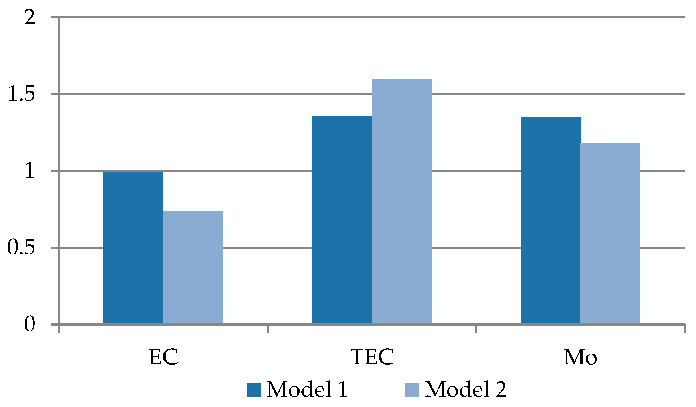
is the change in the output-oriented measure of technical efficiency between periods t and (t+1), and it shows how the ratio of actual outputs to potential has changed. EC indicates the capability of a DMU to catch up with more efficient DMUs.
The second factor in Equation (2) is technological change (
):
is the potential index—the geometric mean of two relations—that characterizes the shift of the potential technology frontier between period t6 and (t + 1). In other words, the last relation reflects a change in the technological efficiency of the evaluated object caused by a shift in the effective boundary.
Another process of technical efficiency decomposition is based on using both CRS and VRS DEA frontiers. A scale efficiency change (
SEC) can be represented as follows:
A pure efficiency change (
PEC) is given below:
The TFP index can be represented in the form of such factors as the change in efficiency and the technical change. Let for a time period t, t = 1, …, T, DMUi, i = 1, …, N, use P inputs to produce S outputs. In a particular time period t, the following definitions hold:
yi is a S×1 vector of output quantities for the DMUi.
xi is a P×1 vector of input quantities for the DMUi.
Y is a N×S matrix of output quantities for all N DMUi.
X is a N×P matrix of input quantities for all N DMUi.
λ is a N×1 vector of weights.
is a scalar.
To calculate
, it is necessary to solve the following linear programming problems [
44]:
The above Equations (12)–(15) need to be solved for each DMU in a sample. Hence, the total number of linear programming problems for N DMUs and T time periods is .
