Abstract
Skeletons are well-known descriptors used for analysis and processing of 2D binary images. Recently, dense skeletons have been proposed as an extension of classical skeletons as a dual encoding for 2D grayscale and color images. Yet, their encoding power, measured by the quality and size of the encoded image, and how these metrics depend on selected encoding parameters, has not been formally evaluated. In this paper, we fill this gap with two main contributions. First, we improve the encoding power of dense skeletons by effective layer selection heuristics, a refined skeleton pixel-chain encoding, and a postprocessing compression scheme. Secondly, we propose a benchmark to assess the encoding power of dense skeletons for a wide set of natural and synthetic color and grayscale images. We use this benchmark to derive optimal parameters for dense skeletons. Our method, called Compressing Dense Medial Descriptors (CDMD), achieves higher-compression ratios at similar quality to the well-known JPEG technique and, thereby, shows that skeletons can be an interesting option for lossy image encoding.
1. Introduction
Images are created, saved and manipulated every day, which calls for effective ways to compress such data. Many image compression methods exist [1], such as the well-known discrete cosine transform and related mechanisms used by JPEG [2]. On the other hand, binary shapes also play a key role in applications such as optical character recognition, computer vision, geometric modeling, and shape analysis, matching, and retrieval [3]. Skeletons, also called medial axes, are well-known descriptors that allow one to represent, analyze, but also simplify such shapes [4,5,6]. As such, skeletons and image compression methods share some related goals: a compact representation of binary shapes and continuous images, respectively.
Recently, Dense Medial Descriptors (DMD) have been proposed as an extension of classical binary-image skeletons to allow the representation of grayscale and color images [7]. DMD extracts binary skeletons from all threshold sets (luminance, hue, and/or saturation layers) of an input image and allows the image to be reconstructed from these skeletons. By simplifying such skeletons and/or selecting a subset of layers, DMD effectively acts as a dual (lossy) image representation method. While DMD was applied for image segmentation, small-scale detail removal, and artistic modification [7,8,9], it has not been used for image compression. More generally, to our knowledge, skeletons have never been used so far for lossy compression of grayscale or color images.
In this paper, we exploit the simplification power of DMD for image compression, with two contributions. First, we propose Compressing Dense Medial Descriptors (CDMD), an adaptation of DMD for lossy image compression, by searching for redundant information that can be eliminated, and also by proposing better encoding and compression schemes for the skeletal information. Secondly, we develop a benchmark with both natural and synthetic images, and use it to evaluate our method to answer the following questions:
- What kinds of images does CDMD perform on best?
- What is CDMD’s trade-off between reconstructed quality and compression ratio?
- Which parameter values give best quality and/or compression for a given image type?
- How does CDMD compression compare with JPEG?
The joint answers to these questions, which we discuss in this paper, show that CDMD is an effective tool for both color and grayscale image compression, thereby showing that medial descriptors are an interesting tool to consider, and next refine, for this task.
The remainder of the paper is organized as follows. Section 2 introduces DMD, medial descriptors, and image quality metrics. Section 3 details our proposed modifications to DMD. Section 4 describes our evaluation benchmark and obtained results. Section 5 discusses our results. Finally, Section 6 concludes the paper.
2. Related work
2.1. Medial Descriptors and the DMD Method
We first introduce the DMD method (see Figure 1). To ease presentation, we consider only grayscale images here. However, DMD can also handle color images by considering each of the three components of an Luv or RGB space in turn (see next Section 4). Let be an 8-bit grayscale image.
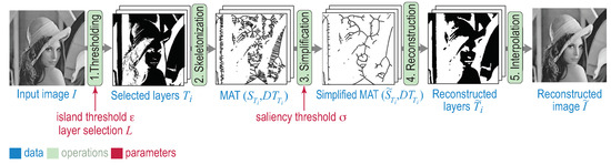
Figure 1.
Dense medial descriptor (DMD) computation pipeline.
The key idea of DMD is to use 2D skeletons to efficiently encode isoluminant structures in an image. Skeletons can only be computed for binary shapes, so I is first reduced to n (256 for 8-bit images) threshold sets (see Figure 1, step 1) defined as
Next, a binary skeleton is extracted from each . Skeletons, or medial axes, are well-known shape descriptors, defined as the locus of centers of maximal disks contained in a shape [10,11,12]. Formally, for a binary shape with boundary , let
be its distance transform. The skeleton of is defined as
where and are the so-called feature points of skeletal point [13]. The pair , called the Medial Axis Transform (MAT), allows an exact reconstruction of as the union of disks centered at having radii . The output of DMD’s second step is hence a set of n MATs for all the layers (Figure 1, step 2). For a full discussion of skeletons and MATs, we refer to [4].
Computing skeletons of binary images is notoriously unstable and complex [4,5]. They contain many so-called spurious branches caused by small perturbations along . Regularization eliminates such spurious branches which, in general, do not capture useful information. Among the many regularization methods, so-called collapsed boundary length ones are very effective in terms of stability, ease of use, and intuitiveness of parameter setting [14,15,16,17]. These compute simplified skeletons by removing from S all points whose feature points subtend a boundary fragment of length shorter than a user-given threshold . This replaces all details along which are shorter than by circular arcs. However, this ‘rounds off’ salient (i.e., sharp and large-scale) shape corners, which is perceptually undesirable. A perceptually better regularization method [13] replaces by
Skeleton points with below a user-defined threshold are discarded, thereby disconnecting spurious skeletal branches from the skeleton rump. The final regularized is then the largest connected component in the thresholded skeleton. Note that Equation (4) defines a saliency metric on the skeleton, which is different from existing saliency metrics on the image, e.g., [18,19].
Regularized skeletons and their corresponding MATs can be efficiently computed on the CPU [17] or on the GPU [7]. GPU methods can skeletonize images up to pixel resolution in a few milliseconds, allowing for high-throughput image processing applications [8,20] and interactive applications [21]. A full implementation of our GPU regularized skeletons is available [22].
The third step of DMD (see Figure 1) is to compute a so-called regularized MAT for each layer , defined as . Using each such MAT, one can reconstruct a simplified version of each layer (Figure 1, step 4). Finally, a simplified version of the input image I is reconstructed by drawing the reconstructed layers atop each other, in increasing order of luminance i, and performing bilinear interpolation between them to remove banding artifacts (Figure 1, step 5). For further details, including implementation of DMD, we refer to [7].
2.2. Image Simplification Parameters
DMD parameterizes the threshold-set extraction and skeletonization steps (Section 2.1) to achieve several image simplification effects, such as segmentation, small-scale detail removal, and artistic image manipulation [7,8,9]. We further discuss the roles of these parameters, as they crucially affect DMD’s suitability for image compression, which we analyze next in Section 3, Section 4 and Section 5.
Island removal: During threshold-set extraction, islands (connected components in the image foreground or background ) smaller than a fraction of , respectively , are filled in, respectively removed. Higher values yield layers having fewer small-scale holes and/or disconnected components. This creates simpler skeletons which lead to better image compression. However, too high values will lead to oversimplified images.
Layer selection: As noted in [7], one does not need all layers to obtain a perceptually good reconstruction of the input I. Selecting a small layer subset of layers from the n available ones leads to less information needed to represent , so better compression. Yet, too few layers and/or suboptimal selection of these degrades the quality of . We study how many (and which) layers are needed for a good reconstruction quality in Section 3.1.
Skeleton regularization: The intuition behind saliency regularization (Equation (4)) follows a similar argument as for layer selection: One can obtain a perceptually good reconstruction , using less information, by only keeping skeletal branches above a certain saliency . Yet, how the choice of affects reconstruction quality has not been investigated, neither in the original paper proposing saliency regularization [13] nor by DMD. We study this relationship in Section 4.
2.3. Image Compression Quality Metrics
Given an image I and its compressed version , a quality metric measures how perceptually close is to I. Widely used choices include the mean squared error (MSE) and peak signal-to-noise ratio (PSNR). While simple to compute and having clear physical meanings, they tend not to match perceived visual quality [23]. The structural similarity (SSIM) index [24] alleviates this by measuring, pixel-wise, how similar two images are by considering quality as perceived by humans. The mean SSIM (MSSIM) is a real-valued quality index that aggregates SSIM by averaging over all image pixels. MSSIM was extended to three-component SSIM (3-SSIM) by applying non-uniform weights to the SSIM map over three different region types: edges, texture, and smooth areas [25]. Multiscale SSIM (MS-SSIM) [26] is an advanced top-down interpretation of how the human visual system interprets images. MS-SSIM provides more flexibility than SSIM by considering variations of image resolution and viewing conditions. As MS-SSIM outperforms the best single-scale SSIM model [26], we consider it next in our work.
2.4. Image Compression Methods
Many image compression methods have been proposed in the literature, with a more recent focus on compressing special types of images, e.g., brain or satellite [1,27]. Recently, deep learning methods have gained popularity showing very high (lossy) compression rates and good quality, usually measured via PSNR and/or MS-SSIM [28,29,30,31,32]. However, such approaches require significant training data and training computational effort and can react in hard to predict ways to unseen data (images that are far from the types present during training). Our method, described next, does not aim to compete with the compression rates of deep learning techniques. However, its explicit ‘feature engineering’ approach offers more control to how images are simplified during compression, is fast, and does not require training data. Separately, technique-wise, our contribution shows, for the first time, that medial descriptors are a useful and usable tool for image compression.
Saliency metrics have become increasingly interesting in image compression [33,34]. Such metrics capture zones in an image deemed to be more important (salient) to humans into a so-called saliency map and use this to drive compression with high quality in those areas. Many saliency map computations methods exist, e.g., [35,36,37,38]; for a good survey thereof, we refer to [34]. While conceptually related, our approach is technically different, since (1) we compute saliency based on binary skeletons (Equation (4)); (2) our saliency thresholding (computation of , Section 2.1) both detects salient image areas and simplifies the non-salient ones; and (3) as explained earlier, we use binary skeletons for this rather than analyzing the grayscale or color images themselves.
3. Proposed Compression Method
Our proposed Compressing Dense Medial Skeletons (CDMD) adapt the original DMD pipeline (Figure 1) to make it effective for image compression in two directions: layer selection (Section 3.1) and encoding the resulting MAT (Section 3.2), as follows.
3.1. Layer Selection
DMD selects a subset of layers from the total set of n layers based on a simple greedy heuristic: Let be the reconstruction of image I using all layers, except . The layer yielding the smallest reconstruction error is deemed the least relevant and thus first removed. The procedure is repeated over the remaining layers, until only L layers are left. This approach has two key downsides: Removing the least-relevant layer (for reconstruction) at a time does not guarantee that subsequent removals do not lead to poor quality. For an optimal result, one would have to maximize quality over all combinations of L (kept) layers selected from n, which is prohibitively expensive. Secondly, this procedure is very expensive, as it requires reconstructions and image comparisons to be computed.
We improve layer selection by testing three new strategies, as follows.
Histogram thresholding: We compute a histogram of how many pixels each layer individually encodes, i.e., . Next, we select all layers having values above a given threshold. To make this process easy, we do a layer-to-threshold conversion: given a number of layers L to keep, we find the corresponding threshold based on binary search.
Histogram local maxima: Histogram thresholding can discard layers containing small but visually important features such as highlights. Furthermore, all layers below the threshold are kept, which does not lead to optimal compression. We refine this by finding histogram local maxima (shown in Figure 2b for the test image in Figure 2a). The intuition here is that the human eye cannot distinguish subtle differences between adjacent (similar-luminance) layers [39], so, from all such layers, we can keep only the one contributing the most pixels to the reconstruction. As Figure 2c shows, 15 layers are enough for a good-quality reconstruction, also indicated by a high MS-SSIM score.
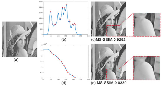
Figure 2.
Layer selection methods. (a) Original image. (b) Histogram of (a), with local maxima marked in red. (c) Reconstruction of (a) using 15 most relevant layers given by (b). (d) Cumulative histogram of (a), with selected layers marked red. (e) Reconstruction of (a) using the 15 most relevant layers given by (d).
Cumulative histogram: We further improve layer selection by using a cumulative layer histogram (see Figure 2d for the image in Figure 2a). We scan this histogram left to right, comparing each layer with layer , where m is the minimally-perceivable luminance difference to a human eye (set empirically to 5 [39] on a luminance range of ). If the histogram difference between layers and is smaller than a given threshold , we increase j until the difference is above . At that point, we select layer and repeat the process until we reach the last layer. However, setting a suitable is not easy for inexperienced users. Therefore, we do a layer-to-threshold conversion by a binary search method, as follows. Let be the range of the cumulative histogram. At the beginning of the search, this range equals . We next set and compare the number of layers produced under this condition with the target, i.e. desired, user-given value L. If , then the search ends with the current value of . If , we continue the search in the lower half of the current range. If , we continue the search in the upper half of the current range. Since L is an integer value, the search may sometimes oscillate, yielding values that swing around, but do not precisely equal, the target L. To make the search end in such situations, we monitor the computed over subsequent iterations and, if oscillation, i.e., a non-monotonic evolution of the values over subsequent iterations, is detected, we stop the search and return the current . Through this conversion, what users need to set is only the desired number of layers, which makes it simple to use by any target group – much like setting the ‘quality’ parameter in typical JPEG compression. Compared to local maxima selection, the cumulative histogram method selects smoother transition layers, which yields a better visual effect. For example, in Figure 2c, the local details around the shoulder show clear banding effects; the same region is much smoother when cumulative histogram selection is used (Figure 2e). Besides improved quality, cumulative histogram selection is simpler to implement and use, as it does not require complex and/or sensitive heuristics for detecting local maxima.
Figure 3 compares the four layer selection methods discussed above. We test these on a 100-image database with 10 different image types, each having 10 images (see Table 1). The 10 types aim to capture general-purpose imagery (people, houses, scenery, animals, paintings) which are typically rich in details and textures; images having a clear structure, i.e., few textures, sharp contrasts, well-delineated shapes shapes (ArtDeco, cartoon, text); and synthetic images being somewhere between the previous two types (scientific visualization).
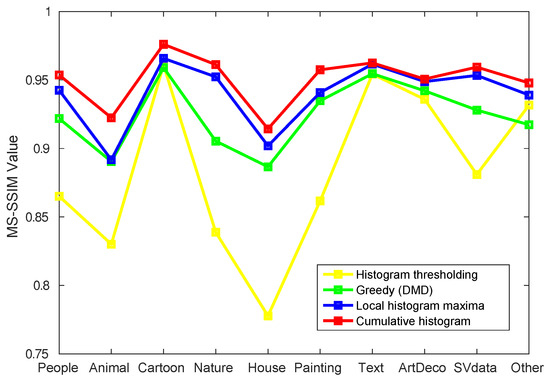
Figure 3.
Average MS-SSIM scores for four layer selection methods (30 layers selected) for images in ten different classes. The cumulative histogram method performs the best and is hence used in CDMD.

Table 1.
The benchmark of 100 images (available at [40]) used throughout this work for testing CDMD.
Average MS-SSIM scores show that the cumulative histogram selection yields the best results for all image types, closely followed by local maxima selection and next by the original greedy method in DMD. The naive histogram thresholding yields the poorest MS-SSIM scores, which also strongly depend on image type. Besides better quality, the cumulative histogram method is also dramatically faster, 3000 times more than the greedy selection method in [7]. Hence, cumulative histogram is our method of choice for layer selection for CDMD.
3.2. MAT Encoding
MAT computation (Section 2.1) delivers, for each selected layer , pairs of skeletal pixels with corresponding inscribed circle radii . Naively storing this data requires two 16-bit integer values for the two components of and one 32-bit floating-point value for r, respectively. We propose next two strategies to compress this data losslessly.
Per-layer compression: As two neighbor pixels in a skeleton are 8-connected, their differences in x and y coordinates are limited to , and similarly . Hence, we visit all pixels in a depth-first manner [41] and encode, for each pixel, only the , and values. We further compress this delta-representation of each MAT point by testing ten lossless encoding methods: Direct encoding (use one byte per MAT point in which and take up two bits each, and three bits, i.e., 0xxyyrrr); Huffman [42], Canonical Huffman, Unitary [43], Exponential Golomb, Arithmetic [44], Predictive, Compact, Raw, and Move-to-Front (MTF) [45]. To compare the effectiveness of these methods, we use the compression ratio of an image I defined as
where is the byte-size of the original image I and is the byte-size of the MAT encoding for all selected layers of . Table 2 (top row) compares the 10 tested encoding methods, showing average value for the 10 image types in Figure 3, and 12 different combinations of parameters , L, and per compression-run. The highest value in each row is marked in bold.
Table 2.
Comparison of average compression ratios (Equation (5)) for 10 lossless MAT-encoding methods on 100 images using only per-layer compression (top row) and inter-layer compression (bottom row).
Inter-layer compression: The inter-layer compression leaves, likely, still significant redundancy in the MATs of different layers. To remove this, we compress the MAT of all layers (each encoded using all 10 lossless methods discussed above) with eight lossless-compression algorithms: Lempel–Ziv–Markov Chain (LZMA) [46], LZHAM [47], Brotli [48], ZPAQ [49], BZip2 [50], LZMA2 [46], BSC [51], and ZLib [52], all available in the Squash library [53]. Figure 4 shows boxplots (Equation (5)) for all our 100 test images. Blue boxes show the 25–75% quantile; red lines are medians; black whiskers show extreme data points not considered outliers; outliers are shown by red ‘+’ marks. Overall, ZPAQ is the best compression method, 20.15% better than LZMA, which was used in the original DMD method [7]. Hence, we select ZPAQ for CDMD.
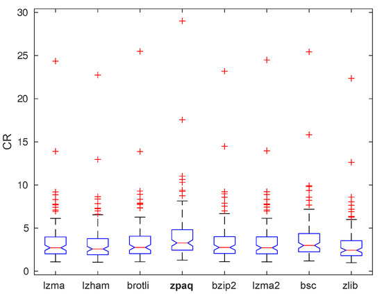
Figure 4.
Compression ratio boxplots for eight compression methods run on 100 images.
Table 2 (second row) shows the average values after applying inter-layer compression. Interestingly, direct encoding turns to be better than the nine other considered lossless encoding methods. This is because the pattern matching of the inter-layer compressor is rendered ineffective when the signal encoding already approaches its entropy. Given this finding, we further improve direct encoding by considering all combinations among possible values of , and . Among the combinations, only 40 are possible as the five cases with cannot exist in practice. This leads to an information content of bits per skeleton pixel instead of bits for direct encoding. Table 2 (rightmost column) shows the average values with the 40-case encoding, which is 6.74% better than the best in the tested methods after all-layer compression. Hence, we keep this encoding method for CDMD.
4. Evaluation and Optimization
Our CDMD method described in Section 3 introduced three improvements with respect to DMD: the cumulative histogram layer selection, the intra-layer compression (40-case algorithm), and the inter-layer compression (ZPAQ). On our 100-image benchmark, these jointly deliver the following improvements:
- Layer selection: 3000 times faster and 3.28% higher quality;
- MAT encoding: 20.15% better compression ratio.
CDMD depends, however, on three parameters: the number of selected layers L, the size of removed islands , and the saliency threshold . Moreover, a compressed image is characterized by two factors: the visual quality that captures how well depicts the original image I, e.g., measured by the MS-SSIM metric, and the compression ratio (Equation (5)). Hence, the overall quality of CDMD can be modeled as
Optimizing this two-variate function of three variables is not easy. Several commercial solutions exist, e.g., TinyJPG [54] but their algorithms are neither public nor transparent. To address this, we first merge the two dependent variables, and , into a single one (Section 4.1). Next, we describe how we optimize for this single variable over all three free parameters (Section 4.2).
4.1. Joint Compression Quality
We need to optimize for both image quality and compression ratio (Equation (6)). These two variables are, in general, inversely correlated: strong compression (high ) means poor image quality (low ), and vice versa. To handle this, we combine and into a single joint quality metric
where is the of a given image I normalized (divided) by the maximal value over all images in our benchmark. The transfer functions and are used to combine (weigh) the two criteria we want to optimize for, namely quality and compression ratio . After extensive experimentation with images from our benchmark, we found that perceptually weighs more than , which motivates the quadratic contribution of the former vs. linear of the latter. Note that, if desired, and can be set to the identity function, which would imply a joint quality Q defined as the mean of the two.
4.2. Optimizing the Joint Compression Quality
To find parameter values that maximize Q (Equation (7)), we fix, in turn, two of the three free parameters L, , and to empirically-determined average values, and vary the third parameter over its allowable range via uniform sampling. The maximum Q value found this way determines the value of the varied parameter. This is simpler, and faster, than the usual hyper-parameter grid-search used, e.g., in machine learning [55], and is motivated by the fact that our parameter space is quite large (three-dimensional) and thus costly to search exhaustively by dense grid sampling. This process leads to the following results.
Number of layers: To study how L affects the joint quality Q, we plot Q as a function of L for our benchmark images. We sample L from 10 to 90 with a step of 10, following observations in [7] stating that 50–60 layers typically achieve good quality. The two other free variables are set to and . Figure 5a shows the results. We see that CDMD works particularly well for images of art deco and scientific visualization types. We also see that Q hardly changes for . Figure 5b summarizes these insights, showing that values give an overall high Q for all image types.
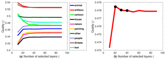
Figure 5.
Quality Q as a function of number of layers L. (a) Q plots per image type. (b) Average Q for all image types. Black dots indicate good L values (20, 30, and 40).
Island size and saliency: We repeat the same evaluation for the other two free parameters, i.e., minimal island size and skeleton saliency , fixing each time the other two parameters to average values. Figure 6 shows how Q varies when changing and over their respective ranges of and , similar to Figure 5. These ranges are determined by considerations outlined earlier in related work [7,8,9,13]. Optimal values for and are indicated in Figure 6 by black dots.
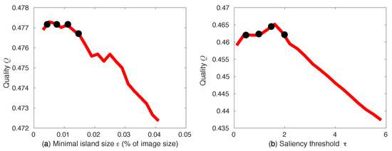
Figure 6.
Quality Q as a function of island size (a) and skeleton saliency simplification (a). Selected optimal parameter values are marked black.
4.3. Trade-Off between MS-SSIM and CR
As already mentioned, our method, and actually any lossy image compression method, has a trade-off between compression (which we measure by ) and quality (which we measure by MS-SSIM). Figure 7 shows the negative, almost-linear, correlation between and MS-SSIM for the 10 house images in our benchmark, with each image represented by a different color. Same-color dots show different settings of L, , and parameters, computed as explained in Section 4.2. This negative correlation is present for both the color version of the test image (Figure 7b) and its grayscale variant (Figure 7a). However, if we compare a set of same-color dots in Figure 7a, i.e., compressions of a given grayscale image for the 48 parameter combinations, with the similar set in Figure 7b, i.e., compressions of the same image, color variant for the same parameter combinations, we see that the first set is roughly lower and more to the left than the second set. That is, CDMD handles color images compressed better than grayscale ones, i.e., yields higher and/or higher MS-SSIM values. Very similar patterns occur for all other nine image types in our benchmark. For full results, we refer to [40].
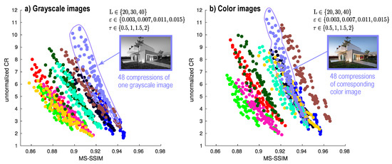
Figure 7.
Trade-off between MS-SSIM and CR on 10 grayscale house images (a) and their corresponding color versions (b). The outlines show the compressions of a single image for 48 parameter combinations.
Besides parameter values, the trade-off between MS-SSIM and CR depends on the image type. Figure 8 shows this by plotting the average MS-SSIM vs for all 10 image types in our benchmark. Here, one dot represents the average values of the two metrics for a given parameter-setting over all images in the respective class. We see the same inverse correlation as in Figure 7. We also see that CDMD works best for art decoration (artDeco) and scientific visualization (SVdata) image types.
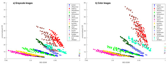
Figure 8.
Average MS-SSIM vs. CR for 10 image types for CDMD (filled dots) and JPEG (hollow dots). Left shows results for the grayscale variants of the color images (shown right).
4.4. Comparison with JPEG
Figure 8 also compares the MS-SSIM and values of CDMD (full dots) with JPEG (hollow dots) for all our benchmark images, for their grayscale versions (a) and color versions (b), respectively. Overall, JPEG yields higher MS-SSIM values, but CDMD yields better values for most of its parameter settings. We also see that CDMD performs relatively better for the color images. Figure 9 further explores this insight by showing ten images, one of each type, from our benchmark, compressed by CDMD and JPEG, and their corresponding CR and MS-SSIM values. Results for the entire 100-image database are available in the supplementary material. We see that, if one prefers a higher over higher image quality, CDMD is a better choice than JPEG. Furthermore, there are two image types for which we get both a higher than JPEG and a similar quality: Art Deco and Scientific Visualization. Figure 10 explores these classes in further detail, by showing four additional examples, compressed with CDMD and JPEG. We see that CDMD and JPEG yield results which are visually almost identical (and have basically identical MS-SSIM values). However, CDMD yields compression values 2 up to 19 times higher than JPEG. Figure 10(a3–d3) shows the per-pixel difference maps between the compressed images with CDMD and JPEG (differences coded in luminance). These difference images are almost everywhere black, indicating no differences between the two compressions. Minimal differences can be seen, upon careful examination of these difference images, along a few luminance contours, as indicated by the few bright pixels in the images. These small differences are due to the salience-based skeleton simplification in CDMD.
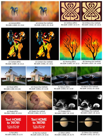
Figure 9.
Comparison of JPEG (a1–j1) with our method (a2–j2) for 10 image types. For each image, we show the MS-SSIM quality and compression ratio .
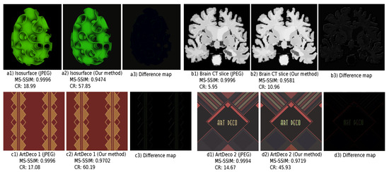
Figure 10.
Our method (a2–d2) yields higher compression than, and visually identical quality with, JPEG (a1–d1) for two image classes: Scientific Visualization (a,b) and Art Deco (c,d)).
For a more detailed comparison with JPEG, we next consider JPEG’s quality setting q. This value, set typically between 10% and 100%, controls JPEG’s trade-off between quality and compression, with higher values favoring quality. Figure 11 compares CDMD for the Scientific Visualization and ArtDeco image types (filled dots) with 10 different settings of JPEG’s q parameter, uniformly spread in the interval (hollow dots). Each dot represents the average of MS-SSIM and CR for a given method and image type for a given parameter combination. We see that CDMD yields higher MS-SSIM values, and for optimal parameters, also yields a much high value. In contrast, JPEG either yields good MS-SSIM or only high , but cannot maximize both.
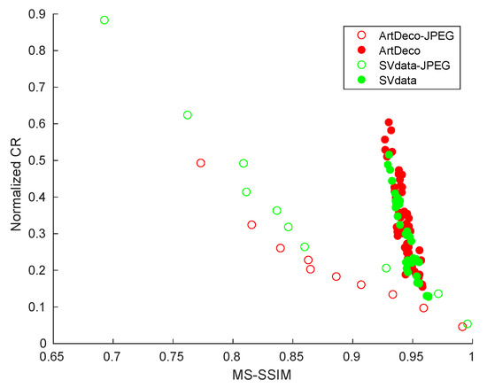
Figure 11.
Average MS-SSIM vs. CR for two image classes (Art Deco, Scientific Visualization), for our method (filled dots) and JPEG (hollow dots).
4.5. Handling Noisy Images
As explained in Section 2.2, the island removal parameter and the saliency threshold jointly ‘simplify’ the compressed image by removing, respectively, small-scale islands and small-scale indentations along the threshold-set boundaries. Hence, it is insightful to study how these parameters affect the compression of images which have high-frequency, small-scale details and/or noise. Figure 12 shows an experiment that illustrates this. An original image was selected which contains high amounts of small-scale high-frequency detail, e.g., the mandrill’s whiskers and fur patterns.
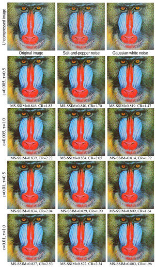
Figure 12.
Results of CDMD on an image with fine-grained detail (left column) additionally corrupted by small-scale noise (middle and right columns), for different values of the and parameters.
The left column shows the CDMD results for four combinations of and . In all cases, we used . As visible, and in line with expectations, increasing and/or has the effect of smoothing out small-scale details, thereby decreasing MS-SSIM and increasing the compression ratio . However, note that contours that separate large image elements, such as the red nose from the blue cheeks, or the pupils from the eyes, are kept sharp. Furthermore, thin-but-long details such as the whiskers have a high saliency, and are thus kept quite well.
The middle column in Figure 12 shows the CDMD results for the same image, this time corrupted by salt-and-pepper noise of density 0.1, compressed with the same parameter settings. We see that the noise is removed very well for all parameter values, the compression results being visually nearly identical to those generated from the uncorrupted image. The MS-SSIM and values are now slightly lower, since, although visually difficult to spot, the added noise does affect the threshold sets in the image. Finally, the right column in Figure 12 shows the CDMD results for the same image, this time corrupted by zero-mean Gaussian white noise with variance 0.01. Unlike salt-and-pepper noise, which is distributed randomly over different locations and has similar amplitudes, the Gaussian noise has a normal amplitude distribution and affects all locations in an image uniformly. Hence, CDMD does not remove Gaussian noise as well as the salt-and-pepper one, as we can see both from the actual images and the corresponding MS-SSIM and values. Yet, even for this noise type, we argue that CDMD does not produce disturbing artifacts in the compressed images, and still succeeds in preserving the main image structures and also a significant amount of the small-scale details.
5. Discussion
We next discuss several aspects of our CDMD image compression method.
Genericity, ease of use: CDMD is a general-purpose compression method for any types of grayscale and color images. It relies on simple operations such as histogram computation and thresholding, as well as on well-tested, robust, algorithms, such as the skeletonization method in [16,17], and ZPAQ. CDMD has three user parameters – the number of selected layers L, island thresholding , and skeleton saliency threshold . These three parameters affect the trade-off between compression ratio and image quality (see Section 4.2). End users can easily understand these parameters as follows: L controls how smooth the gradients (colors or shades) are captured in the compressed image (higher values yield smoother gradients); controls the scale of details that are kept in the image (higher values remove larger details); and controls the scale of corners that are kept in the image (larger values round-off larger corners). Good default ranges of these parameters are given in Section 4.2.
Speed: The most complex operation of the CDMD pipeline, the computation of the regularized skeletons , is efficiently done on the GPU (see Section 2.1). Formally, CDMD’s computational complexity is for an image of R pixels, since the underlying skeletonization is linear in image size, being based on a linear-time distance transform [56]. This is the best that one can achieve complexity-wise. Given this, the CDMD method is quite fast: For images of up to pixels, on a Linux PC with an Nvidia RTX 2060 GPU, layer selection takes under 1 millisecond; skeletonization takes about 1 second per color channel; and reconstruction takes a few hundred milliseconds. Obviously, state-of-the-art image compression methods have highly engineered implementations which are faster. We argue that the linear complexity of CDMD also allows speed-ups to be gained by subsequent engineering and optimization.
Quality vs. compression rate: We are not aware of studies showing how quality and compression rates relate vs. image size for, e.g., JPEG. Still, analyzing JPEG, we see that its size complexity linearly depends on the image size. That is, the compression ratio is overall linear in the input image size R for a given, fixed, quality, since JPEG encodes an image by separate blocks. In contrast, CDMD’s skeletons are of complexity, since they are 1D structures. While a formal evaluation pends, this suggests CDMD may scale better for large image sizes.
Color spaces: As explained in Section 2.1, for color images, (C)DMD is applied to the individual channels of these, following representations in various color spaces. We currently tested the RGB and HSV color spaces, following the original DMD method proposal. For these, we obtained very similar compression vs. quality results. We also tested YUV (more precisely, YCbCr), and obtained compression ratios about twice as high as those reported earlier in this paper (for the RGB space). However, layer selection in the YCbCr space is more delicate than in RGB space: While the U and V channels can be described well with just a few layers (which is good for compression), a slightly too aggressive compression (setting a slightly too low L value) can yield strong visual differences between the original and compressed images. Hence, the method becomes more difficult to control, parameter-wise, by the user. Exploring how to make this control simpler for the end user, while retaining the higher compression rate of the YUV space, is an interesting point for future work.
Best image types: Layer removal is a key factor to CDMD. Images that have large and salient threshold-sets, such as Art Deco and Scientific Visualization, can be summarized by just a few such layers (low L). For instance, the Art Deco image in Figure 10(c1) has only a few distinct gray levels, and large, salient, shapes in each layer. Its CDMD compression (Figure 10(c2)) is of high quality, and is more than 60 times smaller than the original. The JPEG compression of the same image is just 17 times smaller than the original. At the other extreme, we see that CDMD is somewhat less suitable for images with many fine details, such as animal furs and greenery (Figure 9(e2)). This suggests that CDMD could be very well suited (and superior to JPEG) for compressing data-visualization imagery, e.g., in the context of remote/online viewing of medical image databases.
Preprocessing for JPEG: Given the above observation, CDMD and JPEG seem to work best for different types of images. Hence, a valid idea is to combine the two methods rather than let them compete against each other, following earlier work that preprocesses images to aid JPEG’s compression [57]. We consider the same idea, i.e., use CDMD as a preprocessor for JPEG. Figure 13 shows three examples of this combination. When using only JPEG, the original images (a1–c1), at 20% quality (JPEG setting q), yield blocking artifacts (a2–c2). When using JPEG with CDMD preprocessing, these artifacts are decreased (a3–c3). This can be explained by the rounding-off of small-scale noise dents and bumps that the saliency-based skeleton simplification performs [13]. Such details correspond to high frequencies in the image spectrum which next adversely impact JPEG. Preprocessing by CDMD has the effect of an adaptive low-pass filter that keeps sharp and large-scale details in the image while removing sharp and small-scale ones. As Figure 13 shows, using CDMD as preprocessor for JPEG yields a 10% to 20% compression ratio increase as compared to plain JPEG, with a limited loss of visible quality.
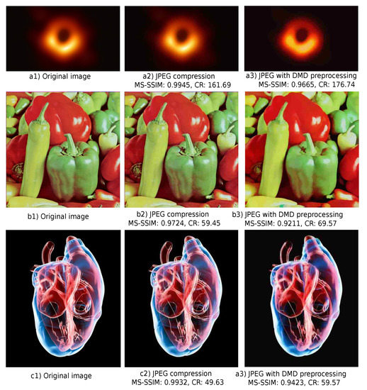
Figure 13.
Comparison of plain JPEG (a2–c2) with CDMD applied as preprocessor to JPEG (a3–c3) for three images.
Limitations: Besides the limited evaluation (on only 100 color images and their grayscale equivalents), CDMD is here only evaluated against a single generic image compression method, i.e., JPEG. As outlined in Section 2.4, tens of other image compression methods exist. We did not perform an evaluation against these since, as already noted, our main research question was to show that skeletons can be used for image compression with good results—something that has not been done so far. We confirmed this by comparing CDMD against JPEG. Given our current positive results, we next aim to improve CDMD, at which point comparison against state-of-the-art image compression methods becomes relevant.
6. Conclusions
We have presented Compressing Dense Medial Descriptors (CDMD), an end-to-end method for compressing color and grayscale images using a dense medial descriptor approach. CDMD adapts the existing DMD method, proposed for image segmentation and simplification, for the task of image compression. For this, we proposed an improved layer-selection algorithm, a lossless MAT-encoding scheme, and an all-layer lossless compression scheme.
To study the effectiveness of our method, we considered a benchmark of 100 images of 10 different types, and did an exhaustive search of the free-parameters of our method, in order to measure and optimize the compression-ratio, perceptual quality, and combination of these two metrics. On a practical side, our evaluation showed that CDMD delivers superior compression to JPEG at a small quality loss; that it delivers both superior compression and quality for specific image types. On a more theoretical (algorithmic) side, CDMD shows, for the first time, that medial descriptors offer interesting and viable possibilities to compress grayscale and color images, thereby extending their applicability beyond the processing of binary shapes.
Several future work directions are possible. First, more extensive evaluations are interesting and useful to do, considering more image types and more compressors, e.g., JPEG 2000, to find the added value of CDMD. Secondly, a low-hanging fruit is using smarter representations of the per-layer MAT: Since skeleton branches are known to be smooth [4], encoding them by higher-level constructs such as splines rather than pixel-chains can yield massive compression-ratio increases with minimal quality losses. We plan to address such open avenues in the near future.
Author Contributions
Conceptualization, A.T.; methodology, J.W. and A.T.; software, M.T. and J.W.; validation, J.W.; analysis, J.W., J.K., and A.T.; investigation, M.T. and J.W.; data curation, J.W.; writing—original draft preparation, J.W.; writing—review and editing, J.K., J.W., and A.T.; visualization, J.W.; supervision, A.T. and J.K. All authors have read and agreed to the published version of the manuscript.
Funding
J. Wang acknowledges the China Scholarship Council (Grant number: 201806320354) for financial support.
Conflicts of Interest
The authors declare no conflict of interest.
References
- Shum, H.Y.; Kang, S.B.; Chan, S.C. Survey of image-based representations and compression techniques. IEEE Trans. Circuits Syst. Video Technol. 2003, 13, 1020–1037. [Google Scholar] [CrossRef]
- Wallace, G.K. The JPEG still picture compression standard. IEEE TCE. 1992, 38, xviii–xxxiv. [Google Scholar] [CrossRef]
- Davies, E.R. Machine Vision: Theory, Algorithms, Practicalities; Academic Press: London, UK, 2004. [Google Scholar]
- Siddiqi, K.; Pizer, S. Medial Representations: Mathematics, Algorithms and Applications; Springer: New York, NY, USA, 2008. [Google Scholar]
- Saha, P.K.; Borgefors, G.; di Baja, G.S. A survey on skeletonization algorithms and their applications. Pattern Recognit. Lett. 2016, 76, 3–12. [Google Scholar] [CrossRef]
- Saha, P.K.; Borgefors, G.; di Baja, G.S. Skeletonization—Theory, Methods, and Application; Academic Press: London, UK, 2017. [Google Scholar]
- Van Der Zwan, M.; Meiburg, Y.; Telea, A. A dense medial descriptor for image analysis. In Proceedings of the International Conference on Computer Vision Theory and Applications(VISAPP-2013), Barcelona, Spain, 21–24 February 2013; pp. 285–293. [Google Scholar]
- Koehoorn, J.; Sobiecki, A.; Boda, D.; Diaconeasa, A.; Doshi, S.; Paisey, S.; Jalba, A.; Telea, A. Automated Digital Hair Removal by Threshold Decomposition and Morphological Analysis. In Proceedings of the International Symposium on Mathematical Morphology and Its Applications to Signal and Image (ISMM), Reykjavik, Iceland, 27–29 May 2015. [Google Scholar]
- Sobiecki, A.; Koehoorn, J.; Boda, D.; Solovan, C.; Diaconeasa, A.; Jalba, A.; Telea, A. A New Efficient Method for Digital Hair Removal by Dense Threshold Analysis. In Proceedings of the 4th World Congress of Dermoscopy, Vienna, Austria, 21 April 2015. [Google Scholar]
- Blum, H. A transformation for extracting new descriptors of shape. In Models for the Perception of Speech and Visual Form; Dunn, W.W., Ed.; MIT Press: Cambridge, UK, 1967; pp. 362–381. [Google Scholar]
- Blum, H.; Nagel, R. Shape description using weighted symmetric axis features. Pattern Recognit. 1978, 10, 167–180. [Google Scholar] [CrossRef]
- Sethian, J.A. A fast marching level set method for monotonically advancing fronts. Proc. Natl. Acad. Sci. USA 1996, 93, 1591–1595. [Google Scholar] [CrossRef]
- Telea, A. Feature Preserving Smoothing of Shapes Using Saliency Skeletons. In Visualization in Medicine and Life Sciences II (VMLS); Springer: Basel, Switzerland, 2012; pp. 153–170. [Google Scholar]
- Ogniewicz, R.L.; Kubler, O. Hierarchic Voronoi skeletons. Pattern Recognit. 1995, 28, 343–359. [Google Scholar] [CrossRef]
- Costa, L.; Cesar, R. Shape Analysis and Classification; CRC Press: New York, NY, USA, 2000. [Google Scholar]
- Falcão, A.; Stolfi, J.; Lotufo, R. The image foresting transform: Theory, algorithms, and applications. IEEE Trans. Pattern Anal. Mach. Intell. 2004, 26, 19–29. [Google Scholar] [CrossRef]
- Telea, A.; van Wijk, J.J. An Augmented Fast Marching Method for Computing Skeletons and Centerlines. In Proceedings of the 2002 Joint Eurographics and IEEE TCVG Symposium on Visualization, VisSym, Barcelona, Spain, 27–29 May 2002. [Google Scholar]
- Kadir, T.; Brady, M. Saliency, Scale and Image Description. Int. J. Comput. Vis. 2001, 45, 83–105. [Google Scholar] [CrossRef]
- Battiato, S.; Farinella, G.M.; Puglisi, G.; Ravi, D. Saliency-based selection of gradient vector flow paths for content aware image resizing. IEEE Trans. Image Process. 2014, 23, 2081–2095. [Google Scholar] [CrossRef]
- Ersoy, O.; Hurter, C.; Paulovich, F.; Cantareiro, G.; Telea, A. Skeleton-based edge bundles for graph visualization. IEEE Trans. Vis. Comput. Graph. 2011, 17, 2364–2373. [Google Scholar] [CrossRef]
- Zhai, X.; Chen, X.; Yu, L.; Telea, A. Interactive Axis-Based 3D Rotation Specification Using Image Skeletons. In Proceedings of the GRAPP, Valletta, Malta, 27–29 February 2020. [Google Scholar]
- Telea, A. Real-Time 2D Skeletonization Using CUDA. Available online: http://www.cs.rug.nl/svcg/Shapes/CUDASkel (accessed on 1 May 2019).
- Wang, Z.; Bovik, A.C. Mean squared error: Love it or leave it? A new look at Signal Fidelity Measures. IEEE Signal Proc. Mag. 2009, 26, 98–117. [Google Scholar] [CrossRef]
- Wang, Z.; Bovik, A.; Sheikh, H.; Simoncelli, E. Image quality assessment: From error visibility to structural similarity. IEEE Trans. Image Process. 2004, 13, 600–612. [Google Scholar] [CrossRef] [PubMed]
- Li, C.; Bovik, A.C. Content-weighted video quality assessment using a three-component image model. J. Electron. Imaging 2010, 19, 110–130. [Google Scholar]
- Wang, Z.; Simoncelli, E.P.; Bovik, A.C. Multiscale structural similarity for image quality assessment. In Proceedings of the Thrity-Seventh Asilomar Conference on Signals, Systems Computers, Pacific Grove, CA, USA, 9–12 November 2003; Volume 2, pp. 1398–1402. [Google Scholar]
- Zhang, C.; Chen, T. A survey on image-based rendering—Representation, sampling and compression. Signal Process Image 2004, 19, 1–28. [Google Scholar] [CrossRef]
- Toderici, G.; O’Malley, S.; Hwang, S.J.; Vincent, D.; Minnen, D.; Baluja, S.; Covell, M.; Sukthankar, R. Variable Rate Image Compression with Recurrent Neural Networks. arXiv 2016, arXiv:1511.06085. [Google Scholar]
- Ballé, J.; Laparra, V.; Simoncelli, E. End-to-end Optimized Image Compression. arXiv 2017, arXiv:1611.01704. [Google Scholar]
- Toderici, G.; Vincent, D.; Johnston, N.; Hwang, S.J.; Minnen, D.; Shor, J.; Covell, M. Full Resolution Image Compression with Recurrent Neural Networks. In Proceedings of the IEEE Conference on Computer Vision and Pattern Recognition, Honolulu, HI, USA, 21–26 July 2017. [Google Scholar]
- Prakash, A.; Moran, N.; Garber, S.; DiLillo, A.; Storer, J. Semantic Perceptual Image Compression using Deep Convolution Networks. In Proceedings of the Data Compression Conference (DCC), Snowbird, UT, USA, 4–7 April 2017. [Google Scholar]
- Stock, P.; Joulin, A.; Gribonval, R.; Graham, B.; Jégou, H. And the Bit Goes Down: Revisiting the Quantization of Neural Networks. arXiv 2019, arXiv:1907.05686. [Google Scholar]
- Guo, C.; Zhang, L. A novel multi resolution spatiotemporal saliency detection model and its applications in image and video compression. IEEE Trans. Image Process. 2010, 19, 185–198. [Google Scholar]
- Andrushia, A.D.; Thangarjan, R. Saliency-Based Image Compression Using Walsh-Hadamard Transform (WHT). In Biologically Rationalized Computing Techniques For Image Processing Applications; Springer: Cham, Switzerland, 2018; pp. 21–42. [Google Scholar]
- Itti, L.; Koch, C.; Niebur, E. A model of saliency-based visual attention for rapid scene analysis. IEEE Trans. Pattern Anal. Mach. Intell. 1998, 20, 1254–1259. [Google Scholar] [CrossRef]
- Imamoglu, N.; Lin, W.; Fang, Y. A saliency detection model using low-level features based on wavelet transform. IEEE Trans. Multimed. 2013, 15, 96–105. [Google Scholar] [CrossRef]
- Lin, R.J.; Lin, W.S. Computational visual saliency model based on statistics and machine learning. J. Vis. 2014, 14, 1–18. [Google Scholar] [CrossRef] [PubMed]
- Arya, R.; Singh, N.; Agrawal, R. A novel hybrid approach for salient object detection using local and global saliency in frequency domain. Multimed. Tools Appl. 2015, 75, 8267–8287. [Google Scholar] [CrossRef]
- Hecht, S. The visual discrimination of intensity and the Weber-Fechner law. J. Gen. Physiol. 2003, 7, 235–267. [Google Scholar] [CrossRef] [PubMed]
- Wang, J. CDMD-Benchmark. Available online: https://github.com/WangJieying/CDMD-benchmark (accessed on 1 May 2020).
- Cormen, T.H.; Stein, C.; Rivest, R.L.; Leiserson, C.E. Introduction to Algorithms, 3rd ed.; MIT Press: London, UK, 2001; pp. 540–549. [Google Scholar]
- Geelnard, M. Basic Compression Library. Available online: github.com/MariadeAnton/bcl/blob/master/src (accessed on 14 January 2015).
- Roy, A.; Scott, A.J. Unitary designs and codes. Des. Codes Cryptogr. 2009, 53, 13–31. [Google Scholar] [CrossRef]
- Langdon, G.G. An Introduction to Arithmetic Coding. IBM J. Res. Dev. 1984, 28, 135–149. [Google Scholar] [CrossRef]
- Bentley, J.L.; Sleator, D.D.; Tarjan, R.E.; Wei, V.K. A Locally Adaptive Data Compression Scheme. Commun. ACM 1986, 29, 320–330. [Google Scholar] [CrossRef]
- Pavlov, I. LZMA SDK (Software Development Kit). Available online: http://www.7-zip.org/sdk.html (accessed on 1 May 2019).
- Geldreich, R. LAHAM. Available online: https://code.google.com/archive/p/lzham/ (accessed on 1 March 2020).
- Alakuijala, J.; Szabadka, Z. Brotli Compressed Data Format. Available online: https://tools.ietf.org/html/rfc7932 (accessed on 1 March 2020).
- Mahoney, M. The Zpaq Compression Algorithm. Available online: http://mattmahoney.net/dc/zpaq_compression.pdf (accessed on 1 March 2020).
- Seward, J. Bzip2. Available online: http://en.wikipedia.org/wiki/Bzip2 (accessed on 1 March 2020).
- Grebnov, I. Libbsc: A High Performance Data Compression Library. Available online: https://github.com/IlyaGrebnov/libbsc (accessed on 1 March 2020).
- Deutsch, P.; Gailly, J. ZLIB Compressed Data Format Specification Version 3.3. Available online: https://datatracker.ietf.org/doc/rfc1950 (accessed on 1 March 2020).
- Nemerson, E. Squash Library. Available online: http://quixdb.github.io/squash (accessed on 1 March 2020).
- TinyJPG. Smart JPEG and PNG Compression. Available online: https://tinyjpg.com (accessed on 1 March 2020).
- Bergstra, J.; Bengio, Y. Random Search for Hyper-Parameter Optimization. J. Mach. Learn. Res. 2012, 13, 281–305. [Google Scholar]
- Cao, T.T.; Tang, K.; Mohamed, A.; Tan, T.S. Parallel banding algorithm to compute exact distance transform with the GPU. In Proceedings of the 2010 ACM SIGGRAPH Symposium on Interactive 3D Graphics and Games, Washington, DC, USA, 19–21 February 2010. [Google Scholar]
- Tushabe, F.; Wilkinson, M.H.F. Image preprocessing for compression: Attribute filtering. In Proceedings of the International Conference on Signal Processing and Imaging Engineering (ICSPIE’07), San Francisco, CA, USA, 24–26 October 2007; pp. 1411–1418. [Google Scholar]
© 2020 by the authors. Licensee MDPI, Basel, Switzerland. This article is an open access article distributed under the terms and conditions of the Creative Commons Attribution (CC BY) license (http://creativecommons.org/licenses/by/4.0/).