Article

Gear Fault Diagnosis through Vibration and Acoustic Signal Combination Based on Convolutional Neural Network

1
School of Mechanical Engineering, Guizhou University, Guiyang 550025, China
2
Key Laboratory of Advanced Manufacturing Technology, Ministry of Education, Guizhou University, Guiyang 550025, China
3
School of Data Science and Information Engineering, Guizhou Minzu University, Guiyang 550025, China
*
Author to whom correspondence should be addressed.
Information 2020, 11(5), 266; https://doi.org/10.3390/info11050266
Submission received: 29 March 2020 / Revised: 23 April 2020 / Accepted: 7 May 2020 / Published: 14 May 2020

Abstract

:
Equipment condition monitoring and diagnosis is an important means to detect and eliminate mechanical faults in real time, thereby ensuring safe and reliable operation of equipment. This traditional method uses contact measurement vibration signals to perform fault diagnosis. However, a special environment of high temperature and high corrosion in the industrial field exists. Industrial needs cannot be met through measurement. Mechanical equipment with complex working conditions has various types of faults and different fault characterizations. The sound signal of the microphone non-contact measuring device can effectively adapt to the complex environment and also reflect the operating state of the device. For the same workpiece, if it can simultaneously collect its vibration and sound signals, the two complement each other, which is beneficial for fault diagnosis. One of the limitations of the signal source and sensor is the difficulty in assessing the gear state under different working conditions. This study proposes a method based on improved evidence theory method (IDS theory), which uses convolutional neural network to combine vibration and sound signals to realize gear fault diagnosis. Experimental results show that our fusion method based on IDS theory obtains a more accurate and reliable diagnostic rate than the other fusion methods.

Graphical Abstract

1. Introduction

With the development of intelligent manufacturing, mechanical equipment has become increasingly sophisticated, which makes the production process increasingly complex. The links between the various components are getting close. Failures at any point can trigger a series of chain reactions with serious consequences. Therefore, the condition monitoring and diagnosis of mechanical equipment is an indispensable means to ensure the safe and reliable operation of the equipment. Only by mastering the health status of the equipment in time can the hidden trouble be found and eliminated effectively by technicians, thereby improving the production efficiency and reducing the economic loss of the enterprise. Mechanical equipment is composed of transmission parts such as shaft, bearing, gear, and belt. As the most typical key component of rotating equipment, gears are in a state of high speed and high load for a long time, and they are most prone to failure, which is widely representative [1]. Therefore, this study aims to investigate the fault diagnosis method of gear.
The traditional fault diagnosis method relies on the vibration signal measured by the acceleration sensor. However, in a high-temperature, high-corrosion and toxic environment, the contact measurement method is limited. Moreover, the fault characterization is not the same because of the diversity of faulty types. In some cases, the vibration characteristics are better than the sound, and in some cases, the opposite is true. Therefore, using non-contact measurement to acquire the sound characteristics of the signal is particularly important. Sound is a wave generated by the vibration of an object, which is transmitted through the air and sensed by the microphone. The non-contact measurement can also reflect the running state of equipment. On the production line, some experienced maintenance technicians can judge the fault by the abnormal sound during the operation of equipment. The vibration and sound signals of the equipment are complementary and mutually enhanced. Lu [2] proposed a sound-field feature extraction method based on acoustic information, which was combined with support vector machine to establish the relationship between sound field characteristics and bearing state and realize fault classification. Zhao [3] proposed a combined acoustic and vibration diagnosis method using acoustic sensors, which effectively improved the correctness and practicability of fault diagnosis of high-voltage circuit breakers. Khazaee [4] proposed an effective method for fault diagnosis of planetary gearbox based on vibration data fusion, which achieved 98% accuracy by means of data fusion. Moosavian [5] analyzed the sound and vibration signals of automotive spark plugs and achieved a fault accuracy of 98.56% based on evidence theory. Othman [6] analyzed different vibration and sound signal processing methods of bearing. The experimental results show that the diagnosis results of combining vibration with sound are better than those of the single signal source.
According to the characteristics of vibration signal of machine, data-driven method, mathematical model and pattern recognition method are widely applied the fault diagnosis [7,8,9]. Convolutional neural network (CNN) is a deep feedforward artificial neural network [10,11]. The CNN automatically learns, extracts and memorizes features from the training set through convolution and pooling, thereby realizing the classification or prediction of test sets, effectively avoiding the dependence on artificial experience, and fully reflecting the inherent relationship between data. Moreover, the CNN is widely used in various fields. In the ImageNet, Krizhevsky [12] used the deep CNN to classify the images and achieved the best results in the competition, which opened the craze for CNN learning. Sermanet [13] used CNN for house identification, using pooling operation to adjust feature weights to make the CNN strong and weak. This method obtained 95.1% classification accuracy on Street View House Number (SVHN) dataset. [14] used CNN for handwriting recognition, enhanced data with elastic deformation. In 2015, Simard [15] designed a ResNet network based on the idea of residual convolution operation, which achieved a recognition rate higher than that of human eyes for the first time in the field of computer vision. In 2016, Aytar [16] proposed the famous SoundNet network, which uses 2D and 1D CNN to extract video and audio features, respectively, which greatly improved the speech recognition rate. In the same year, Silver’s [17] AlphaGo defeated the chess champion Li Shishi, shocked the world, and perfectly presented the highest level of current artificial intelligence. The essence is still CNN. In 2017, Esteva [18] designed a CNN network for diagnosing skin cancer, which reached the level of human experts for the first time and was published in Nature. From the above broad academic achievements, CNN has achieved fruitful results in various fields.
The preceding research shows that the effective fusion of the vibration and sound of the workpiece has a positive effect on the diagnosis of equipment failure. Combined with CNN’s strong recognition capacity, this study takes the gear, which is the most common part of mechanical equipment, as the research object and introduces sound signal on the basis of vibration signals to form multi-source information, which complement each other. In this study, a method that fuses vibration and sound signals is proposed based on IDS theory. A convolutional neural network to implement gearbox fault diagnosis (IGFD-CNN) is used. First, the gearbox fault diagnosis platform is built in a semi-anechoic chamber environment, and vibration and sound signals under different working conditions are collected. Second, an adaptive stacked convolution neural network (ASCNN) is proposed for the vibration signal. In [19], the authors proposed an approach based on the Continuous Wavelet Transform (CWT) for broken bar diagnosis and got great result. According to the conventional feature extraction method, the signal is transformed from the time domain to the time-frequency domain by using wavelet transform in this paper. The time-frequency diagram is sent to the ASCNN model for diagnosis. Third, an end-to-end stacked convolution neural network (ESCNN) is proposed for the sound signal, which avoids background dependence of manual feature extraction. The two steps of feature extraction and fault classification are combined into one model to complete adaptively. The original sound signal is sliced and then directly sent to the ESCNN model. Finally, to solve the limitation of single signal source, which cannot fully reflect the information of the measured object, the multi-sensor fusion algorithm IDS theory is used to further fuse the diagnosis output of vibration and sound signals, and obtain a more accurate and reliable equipment operation state.

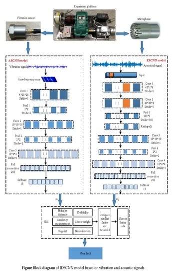
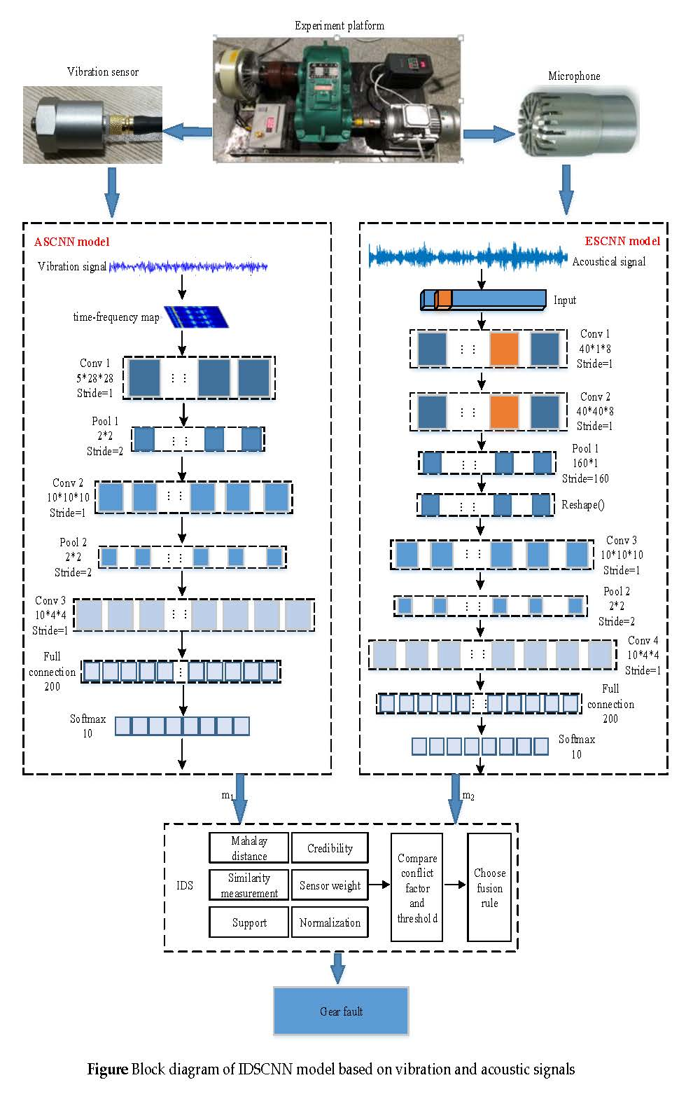
2. Establishing a Diagnostic Model

Four steps in our proposed IGFD-CNN diagnosis model are based on vibration and acoustic signals. In the first part, data acquisition of the original vibration and sound is completed, as shown in Section 3. In the second part, an ASCNN model for gear fault diagnosis based on time-frequency diagram of vibration signal is proposed. The model includes an input layer, three convolutional layers, two sub-sampling layers (pooling layers), a fully connected layer and an output layer. To extract as many local features as possible, a small-scale convolution kernel is used to filter the time-frequency map in the convolutional part. The adaptive feature extraction and dimensionality reduction of the time-frequency map is achieved by the stacking operation of the convolution and pooling layer. Thus, the pattern recognition of gear fault is completed. In the third part, an ESCNN model for gear fault diagnosis based on acoustic signal is proposed. The model includes an input layer, four convolutional layers, two sub-sampling layers, a fully connected layer, and an output layer. Acoustic signals are directly fed into the model, which omits the process of manually extracting features. Feature extraction is completed by the first two convolution layers. The parameters of the ASCNN and ESCNN models are randomly initialized at the beginning of the training. By calculating the error between the predicted and true value during the training process, the error back propagation is used to correct the parameters until the termination condition is satisfied. In addition, the rectified linear unit is used as the activation function followed by each convolutional layer. A batch normalization layer is used to accelerate and improve the learning process of models, and a 50% dropout probability is applied to the fully connected layer to prevent overfitting. After training, the testing dataset is sent to the model. The accuracy of gear fault is obtained by comparing real and predicted labels of the samples. In the fourth part, the output of the ASCNN and ESCNN models are fused using the improved DS theory. (For further theoretical details, please refer to [20]). The diagnosis of the single signal is taken as evidence, and further fusion decision is made to improve the stability and reliability of the running state of gear. The architecture of our proposed IGFD-CNN model is shown in Figure 1.

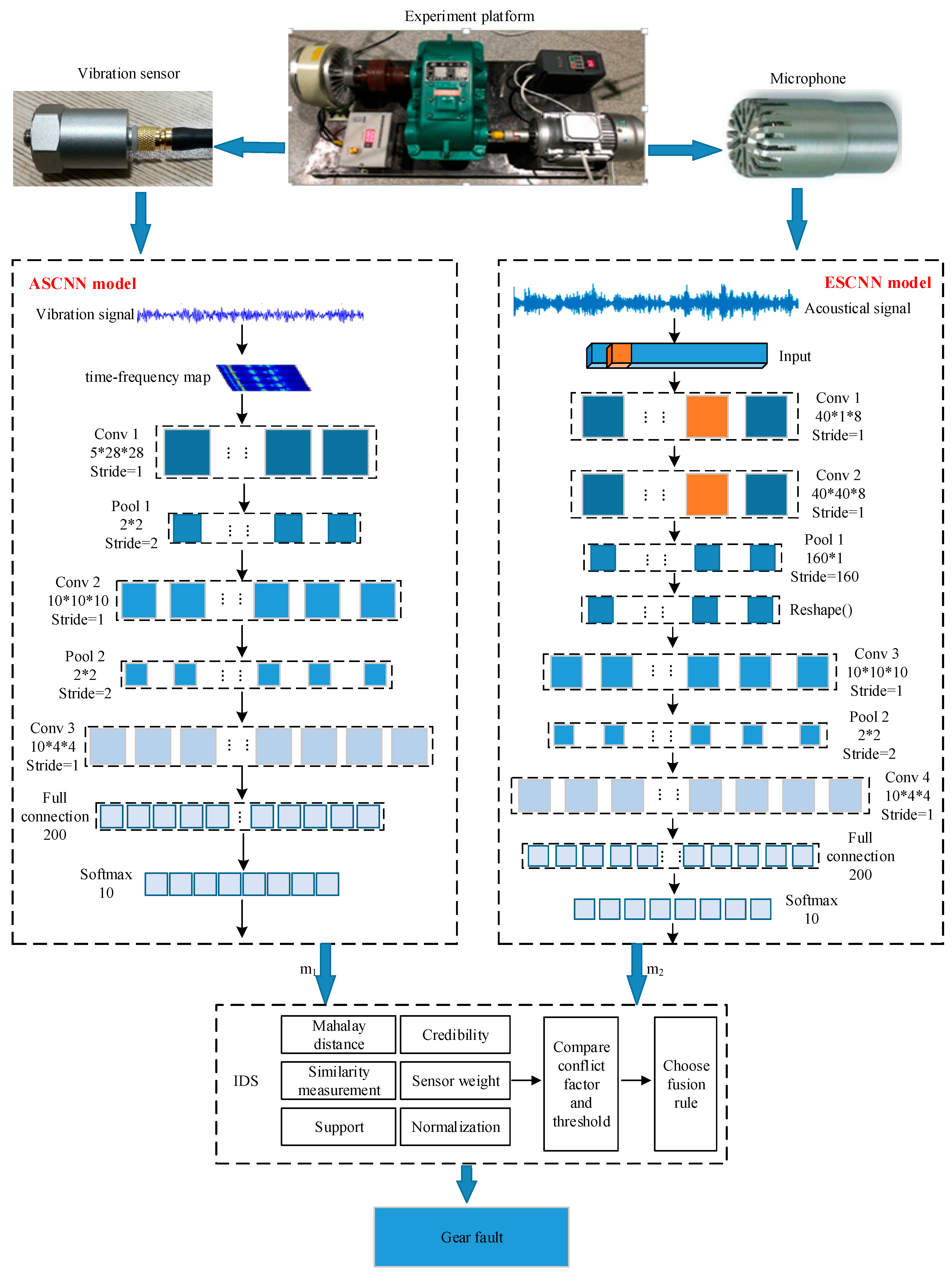
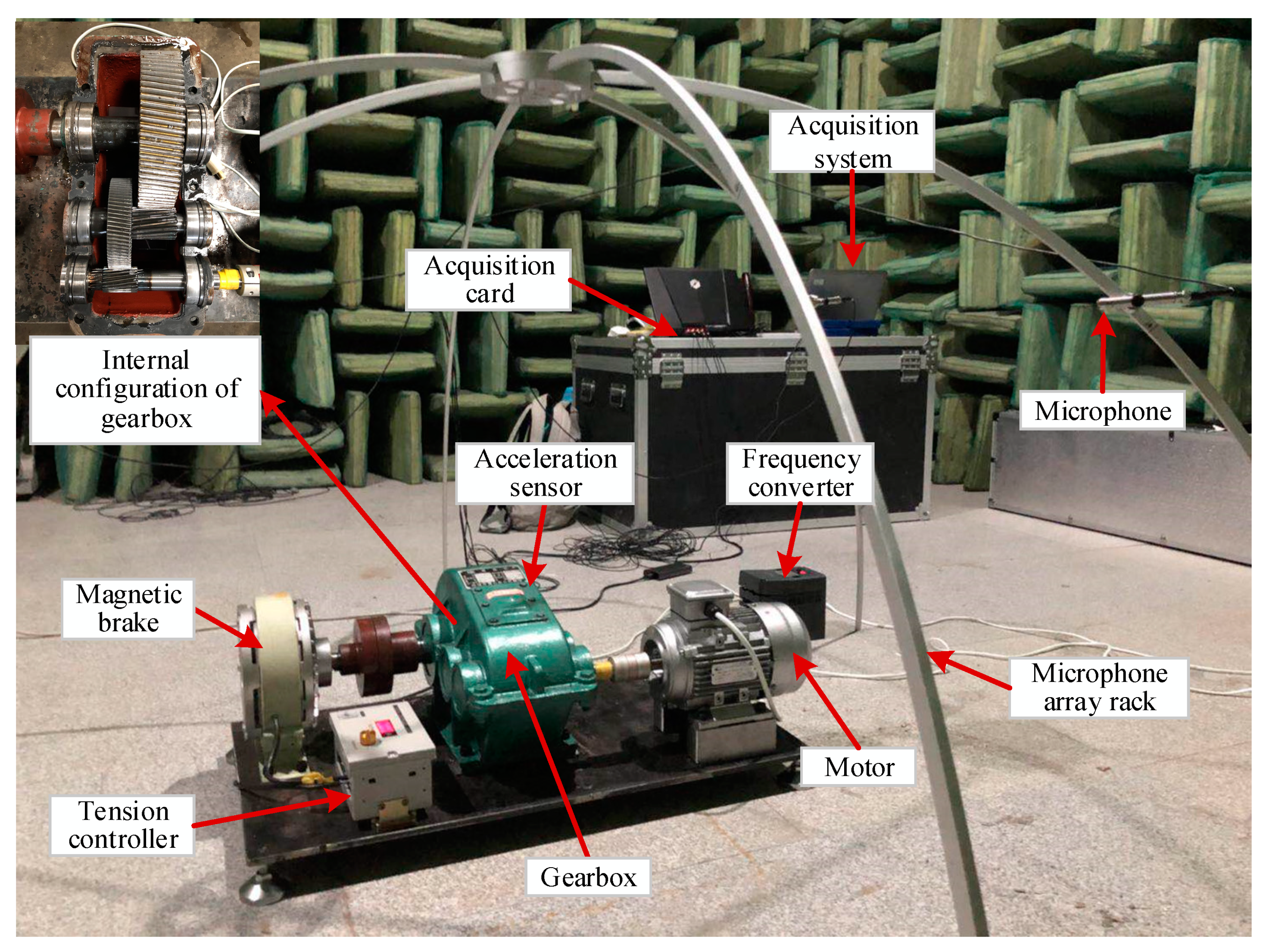
3. Experimental Setup

To verify the effectiveness of the proposed model, the experiments are conducted on a gearbox fault experimental platform in a semi-anechoic room. Figure 2 indicates the composition of the experimental platform and positions for vibration and acoustic sensors. The platform is composed of a two-stage gearbox, a variable frequency motor, a frequency converter, a magnetic brake component, a tension controller, sensor, acquisition card and system [21]. The entire experimental platform is located below the microphone array rack. The 4189-A-021 free-field microphone is fixed on the array frame for collecting acoustic signals of different states of the gear. The CY1010L piezoelectric accelerometer is mounted horizontally on the side of the gearbox for vibration signals. The vibration and acoustic signals are saved in the terminal through data acquisition card for analysis. The top-left corner of Figure 2 shows the internal configuration of the gearbox. In this study, the big gear is selected as the faulty gear. Three fault conditions, including pitting, broken teeth and wear, were set up by the electro discharge machining (EDM) process, as shown in Figure 3. During the process, the entire gear transmission system was driven by a motor. The motor speed was adjusted to 900, 1800 and 2700 r/m to simulate under different working conditions. The load condition was controlled by the magnetic powder brake, and two states were set with load and no-load. The experiment assumed that the interference from other parts of the gearbox was small, and the vibration and acoustic signals measured were considered as only containing gears. The sampling frequency of the vibration and acoustic signal is 12 KHZ and 16 KHZ. The sampling interval is 5 min and the sampling duration is 60 s.
A total of 10 different operating conditions that correspond to the three speeds of the motor were simulated to ensure the diversity of the samples. For a deep learning diagnostic model, the training set is typically used to train the model, and the testing set is used to test the performance of the model. Experimental data are obtained from the raw data by random sampling to objectively evaluate the performance of the proposed model. Three different datasets: vibration, acoustic and hybrid, which are from the no-load condition, were built. The vibration dataset contains 200 samples for each type of gear fault. A total of 75% of the samples were randomly selected as the training set, and the rest was used as the testing set. Thus, the vibration dataset has a total of 2000 samples, including 1500 training samples and 500 testing samples. The acoustic dataset was similarly created. The hybrid dataset is constructed by mixing the vibration and acoustic datasets, which has a total of 4000 samples, including 3000 training samples and 1000 testing samples. Different datasets are selected for training and testing in different models and methods. The description of the dataset is shown in Table 1.

4. Diagnostic Performance Analysis of ASCNN

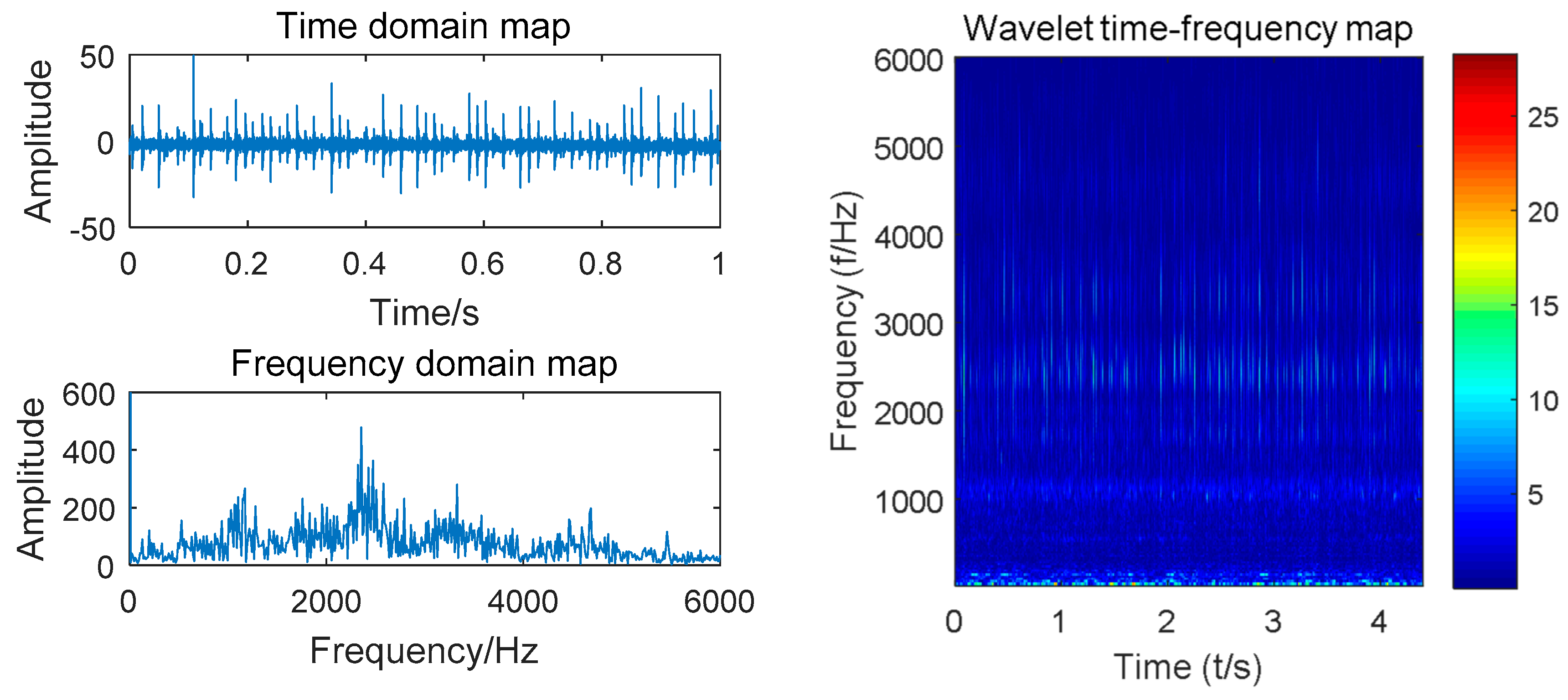
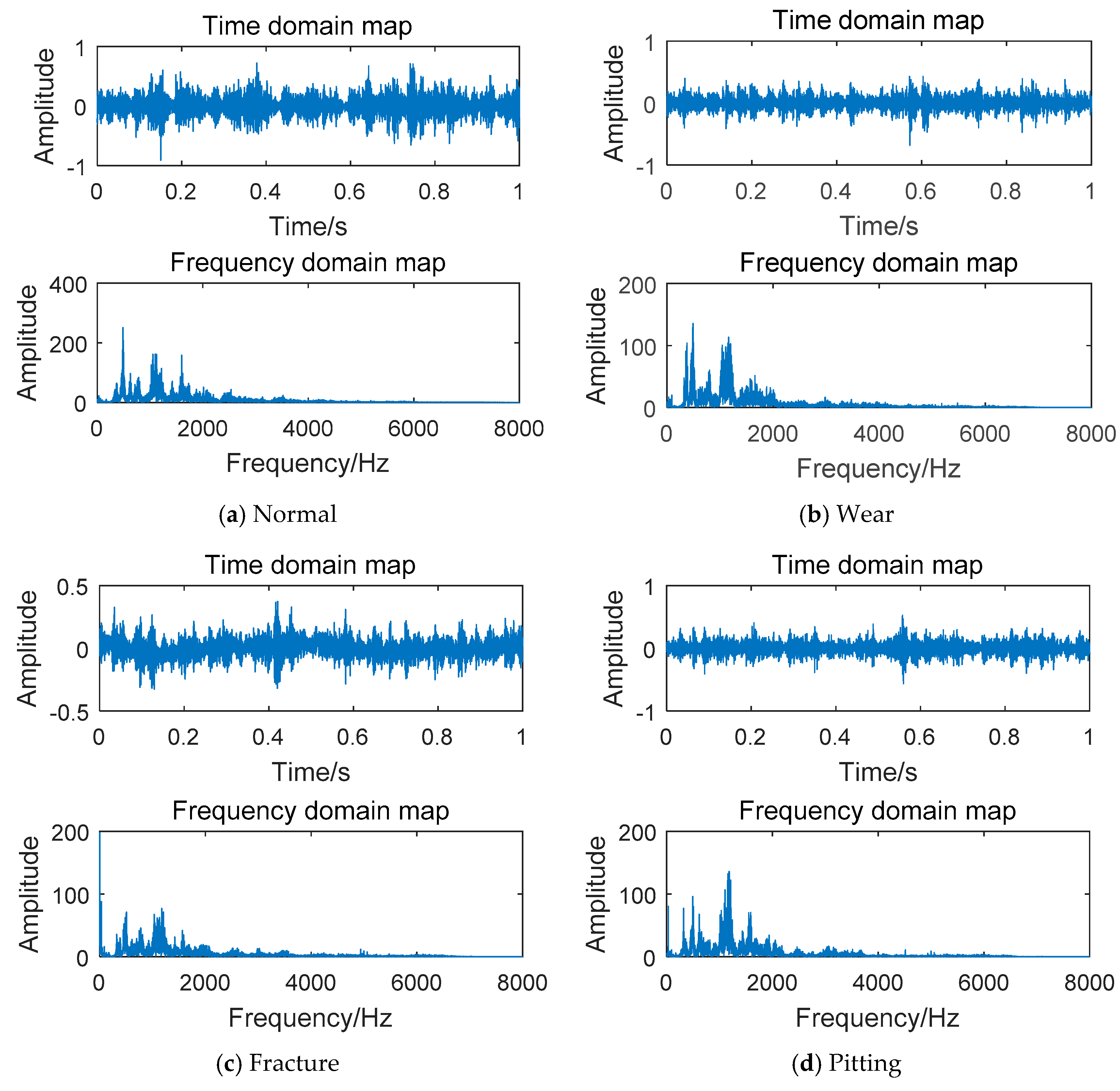
4.1. Feature Extraction

Time domain analysis can only determine whether the vibration value exceeds the standard and cannot determine the location of the vibration. Frequency domain analysis reflects the general information of the signal but not the change of time. Time-frequency analysis maps a 1D time signal to a 2D time scale to see the change in frequency over a small time. Wavelet transform is a new transform analysis method. The transform inherits and develops the idea of STFT localization, overcomes the limitations of fixed window size, and provides a time–frequency window that changes with frequency, which is an ideal tool for time–frequency analysis [22]. A cluster of functions is used instead of the basis functions in the Fourier transform to represent or approximate a signal [23]. Localization analysis of space–time frequencies can be performed by transforming features that can fully highlight certain aspects of the problem. The signal is progressively multi-scale refined by telescopic translation. Finally, the time subdivision at high frequency and frequency subdivision at low frequency can be achieved, which can automatically meet the requirements of analysis and focus on the details of the signal [24].
Taking the vibration signal collected by the experimental platform shown in Figure 2 as an example, we designed 10 gear states with a motor speed of 900 r/min. A sliding window size of 512 with step size of 200 was used to scan the sample. Complex Morlet wavelet with bandwidth parameter and center frequency of 3 was selected for wavelet analysis. The time domain waveform, spectrogram, and time–frequency diagram of the four states of the gear (normal, worn, broken and pitting) are shown in Figure 4, Figure 5, Figure 6 and Figure 7.
Compared with the time domain diagram of Figure 4, Figure 5, Figure 6 and Figure 7, the amplitude of the normal gear is smaller. The fault makes the amplitude larger, and a certain degree of impact is presented, which can monitor the vibration signal. By observing the spectrum of four states, the time domain waveform of the signal has been decomposed into the frequency domain by Fourier transform, and the frequency component and its distribution range of the vibration signal can be obtained. However, the time transformation of a specific component cannot be reflected. The time-frequency diagrams show that the energy of the normal gear is concentrated in the low-frequency band, and the vibration signal arouses the natural frequency of the gear. As the failure occurs, the amplitude is increased, and the impact and meshing of the fault portion excite the medium-high frequency natural vibration of the gear, which exhibits a high frequency band. Intuitively, the time-frequency diagrams of the four states are comparatively similar. Finding out the common characteristics of the same type of fault is necessary. Moreover, distinctions should be made. The powerful image recognition ability of CNN is used to perform gear fault recognition and diagnosis.

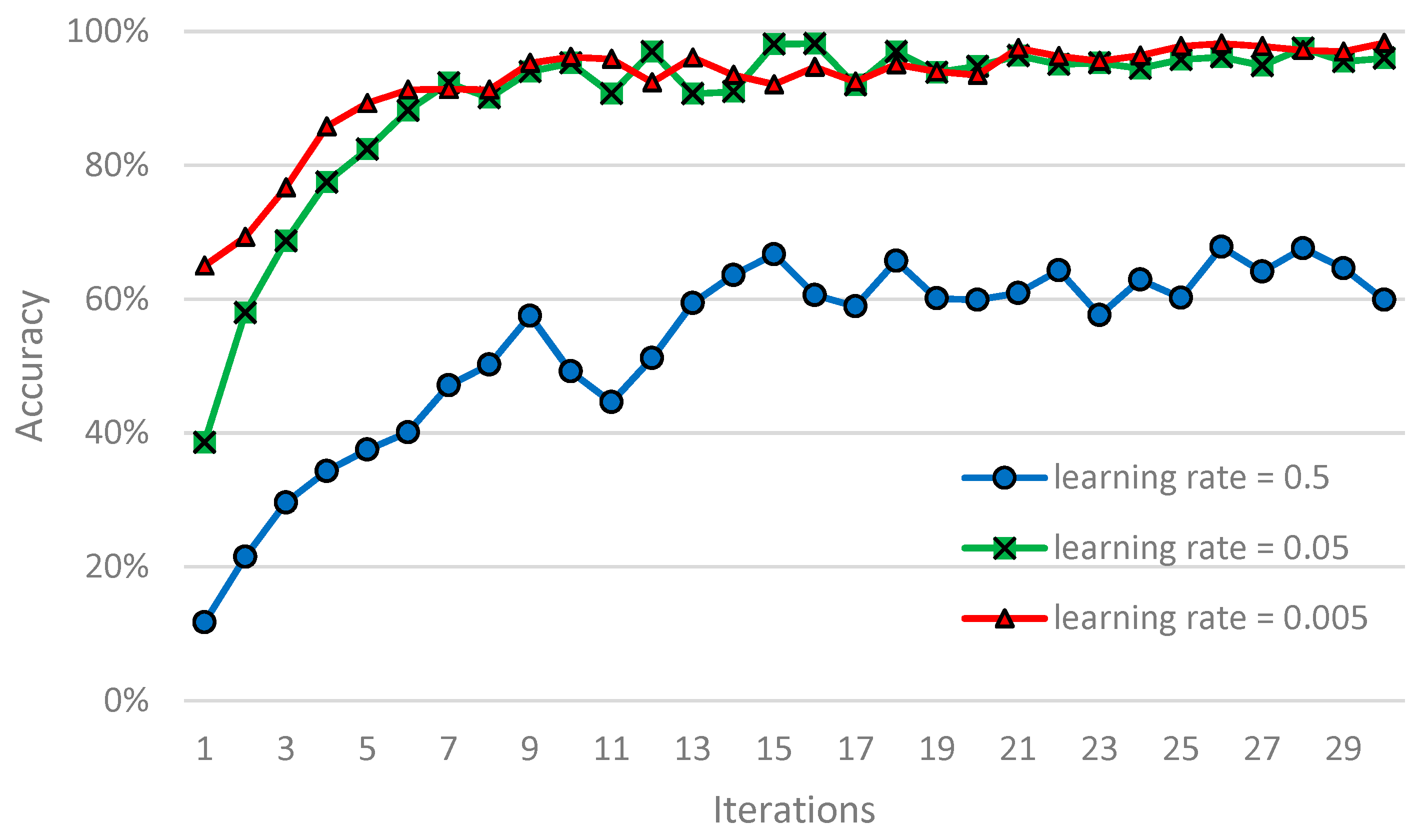
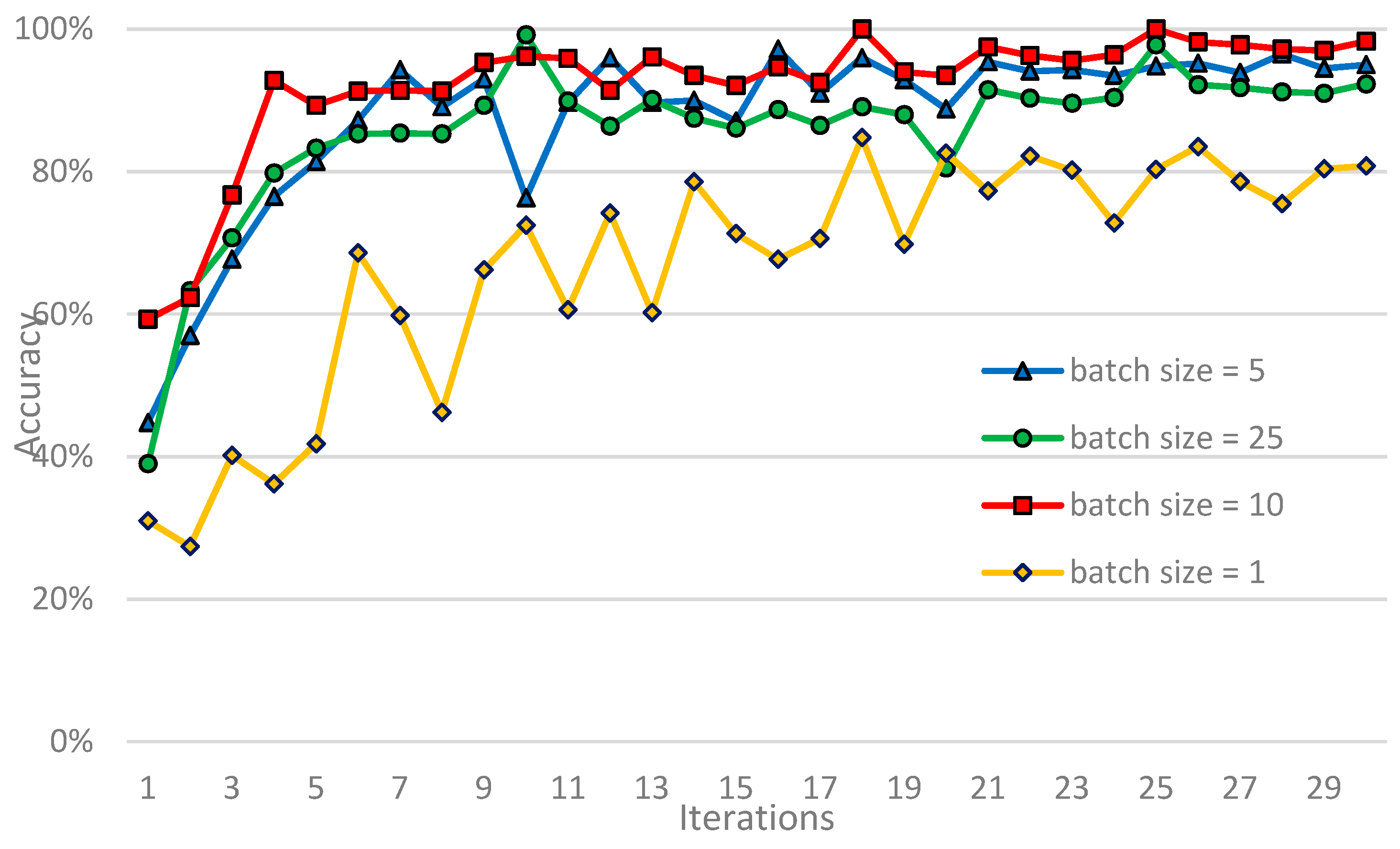
4.2. Parameter Setting

The parameters of CNN have a great influence on the classification accuracy. Our data are derived from the experimental platform and belong to the equilibrium data under artificial interference. Therefore, the accuracy rate is selected as the evaluation index of the model. Parameters that have a large impact on model accuracy include iterations, learning rate and batch size. In the analysis of one of the parameters, an assumption is made that the other two parameters have the fixed value to reduce the complexity.
Iterations. In the training process, the number of iterations is too small to fully learn the features, thereby resulting in underfitting. By contrast, the number of iterations is excessive and the learning is extremely detailed, which results in overfitting. Both of them make the model generalization ability worse. When the iteration is increased to a certain extent, the error is not reduced. However, the time consumption of the system increases as the iteration increases. Therefore, under the premise of error, selecting a suitable iteration can obtain a better fault recognition rate. The learning rate is set to 0.005, the batch size to 10, and the iterations to 50. The relationship between the recognition accuracy of fault and iteration is shown in Figure 8.
Figure 8 shows that the fault recognition accuracy increases as the iteration increases although a slight fluctuation occurred. When the iteration reaches 15, the fault identification accuracy has reached 80%. When the iteration is increased to 30, the accuracy reaches 98%. As the iteration continues to increase, the accuracy tends to be stable. Therefore, 30 is chosen as the iteration of our model.
Learning Rate. Deep learning models are usually trained by a stochastic gradient descent (SGD) algorithm. Learning rate is the gradient coefficient of SGD, which determines the distance of the weight to move in the gradient direction. The SGD has a great influence on the final recognition results. The higher the learning rate is, the faster the learning speed is, which causes the training to not converge or even diverge. The lower the learning rate is, the slower the learning speed is, which makes the training more reliable. However, said training takes a long time. At present, no perfect theoretical support exists for how to select the appropriate learning rate. People usually choose it based on experience. The learning rate is set to 0.5, 0.05, and 0.005. The batch size is set to 10 and the iteration is set to 30, according to the conclusions in the previous section. The relationship between the recognition accuracy of fault and learning rate is shown in Figure 9.
Figure 9 shows that the accuracy of gear box fault identification of ASCNN model is maintained around 60% with a learning rate of 0.5. The curve fluctuates greatly and is extremely unstable. When the learning rate is set to 0.05 and 0.005, the fault recognition rate of the model is maintained around 90%. Relatively speaking, the accuracy of the learning rate of 0.005 is relatively flat and the stability is better. Therefore, a learning rate of 0.005 is the best choice.
Batch size. The batch size is the number of samples that can be processed in one iteration during model training. The larger the batch size is, the faster the convergence speed is, but the likelihood of weight adjustment is reduced. Thus, the recognition accuracy of the model is reduced. The smaller the batch size is, the higher the recognition accuracy of the model is. However, the local optimum is easily achieved, which results in a long system time consumption. The general rule is that the batch size is divisible by the number of samples. Therefore, the batch size in this section is set to 1, 5, 10 and 25. Based on previous results, the learning rate is set to 0.005 and the iteration to 30. The relationship between the recognition accuracy of fault and batch size is shown in Figure 10.
Figure 10 shows that online learning has a batch size of 1. The weight correction direction is based on the gradient direction of the respective samples. Thus, convergence and model recognition accuracy is low. With the increase of batch size, the model converges rapidly and the fluctuation of curve is small. When the batch size is increased from 5 to 10, the recognition accuracy of model increases. However, the accuracy does not rise but drop when the same continues to increase to 25. Therefore, the batch size in this section is set to 10, which is helpful for gearbox fault identification and diagnosis.

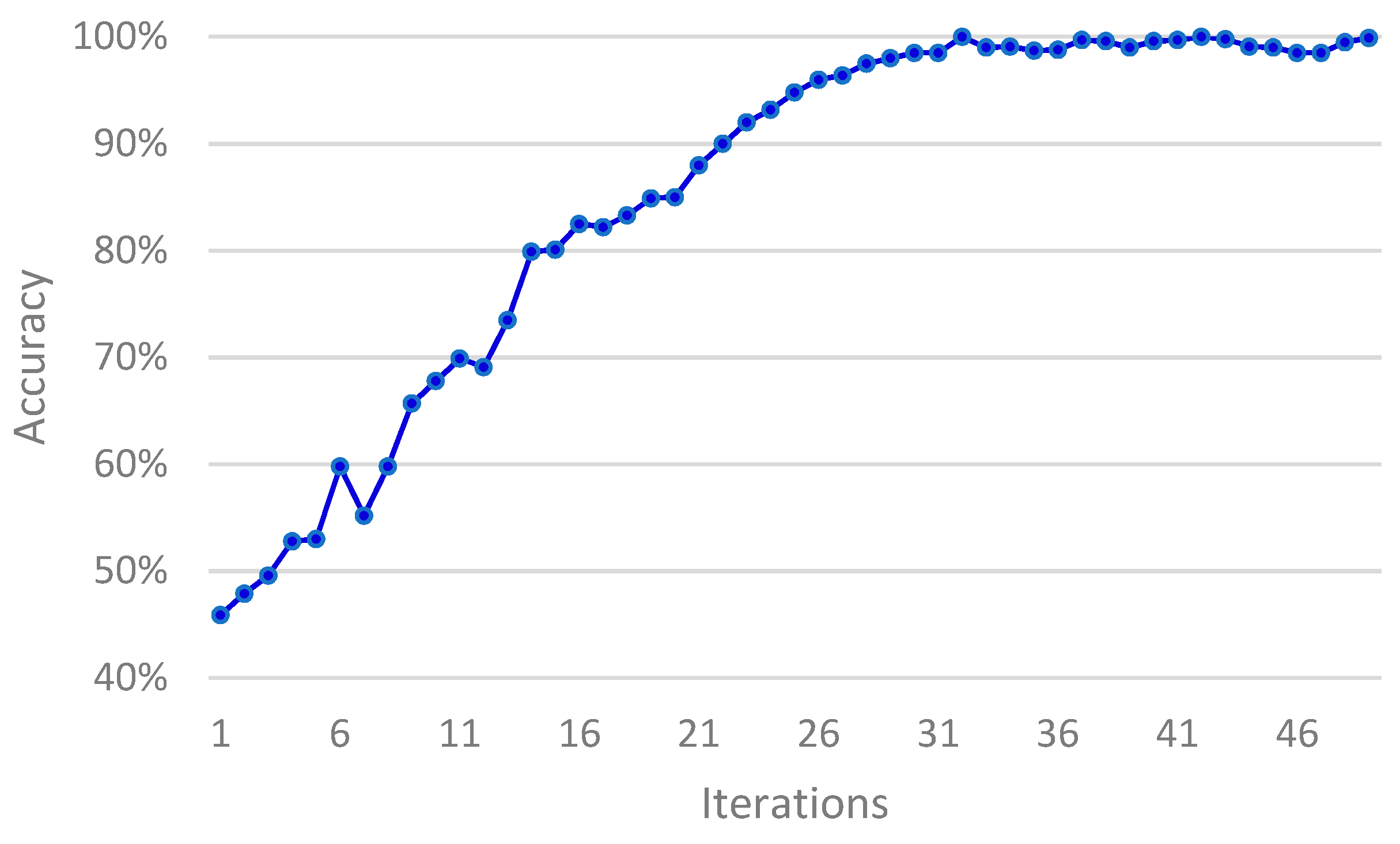
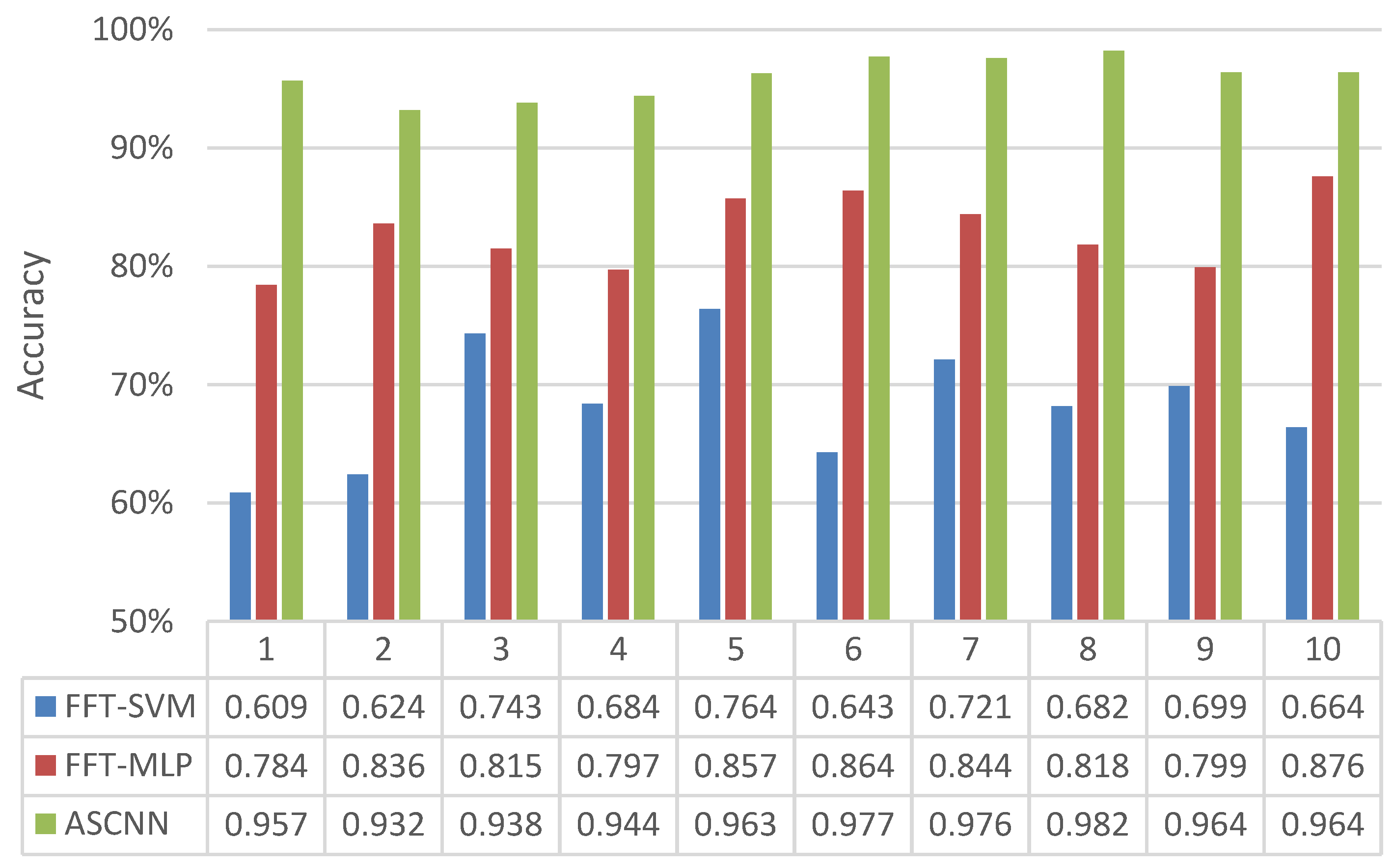
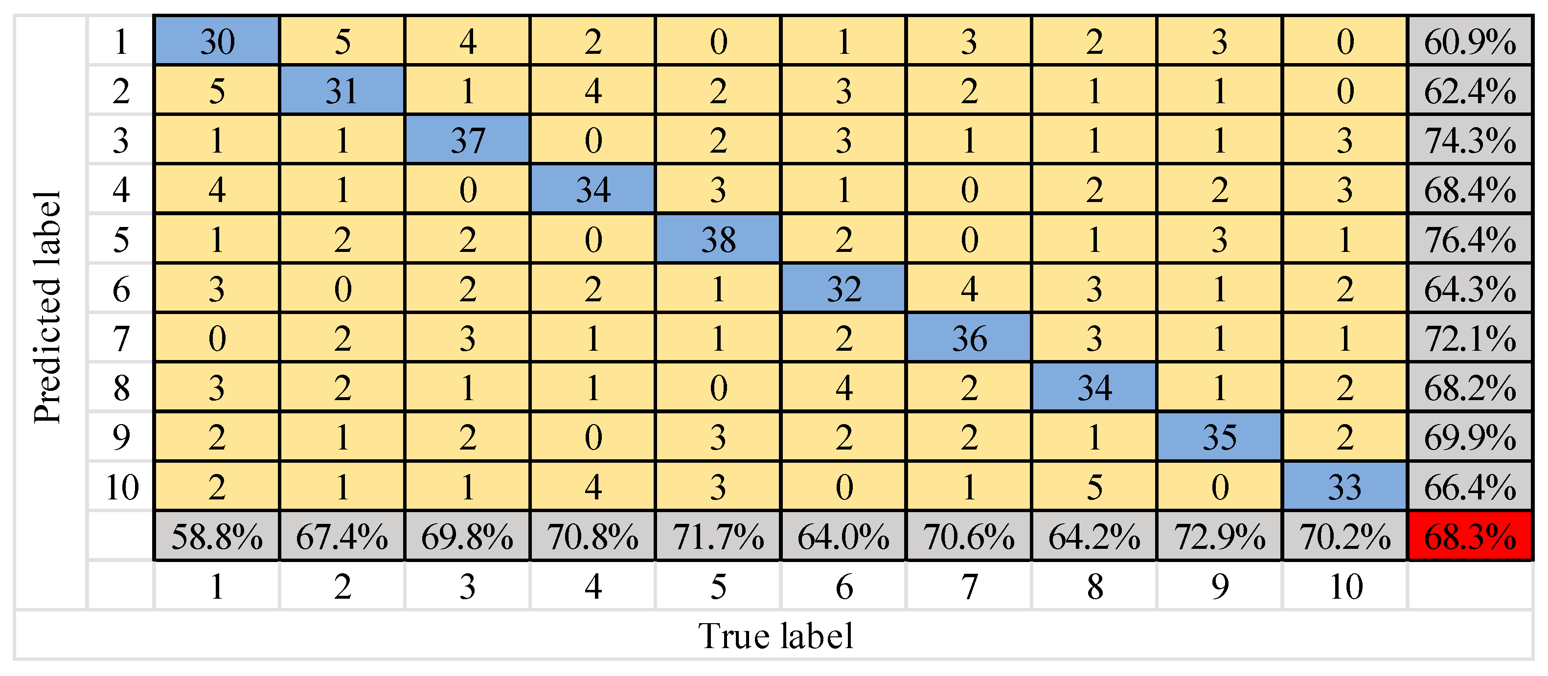
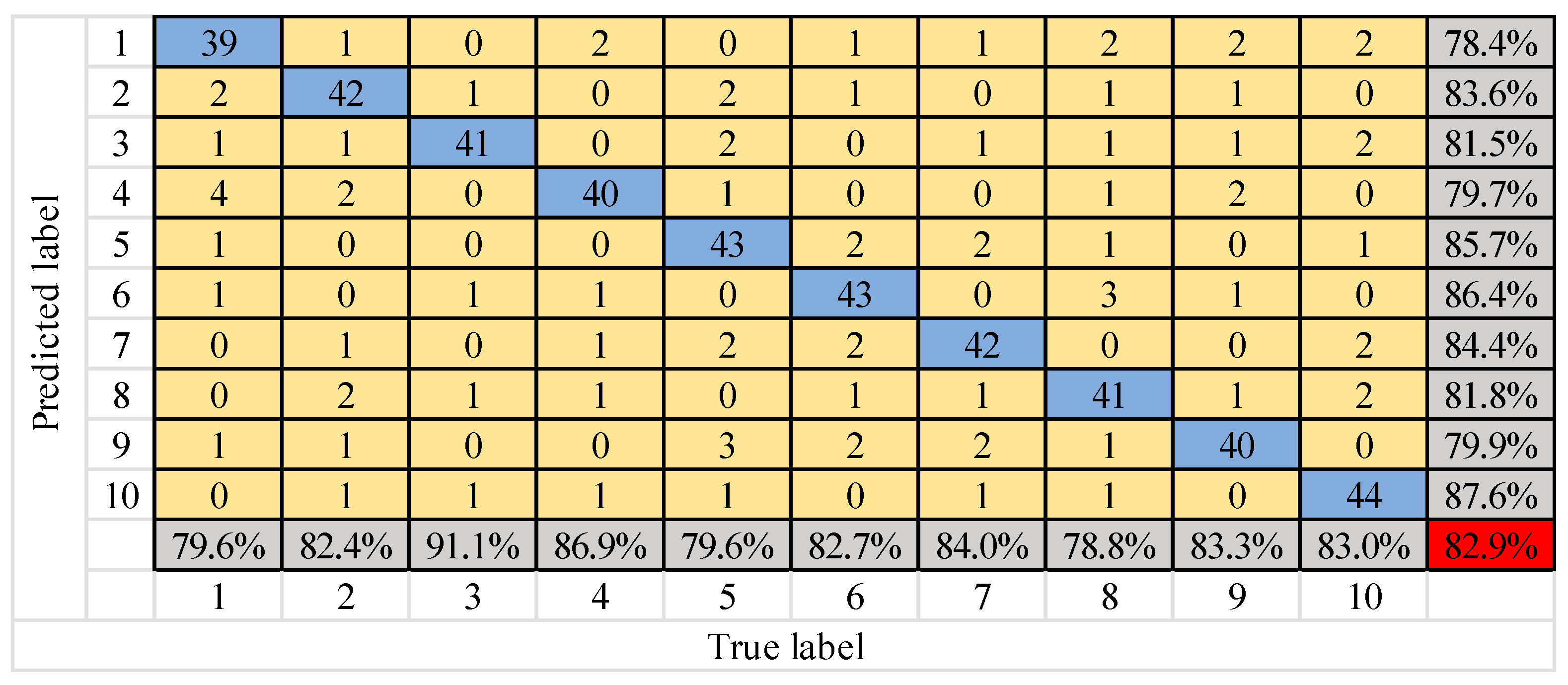
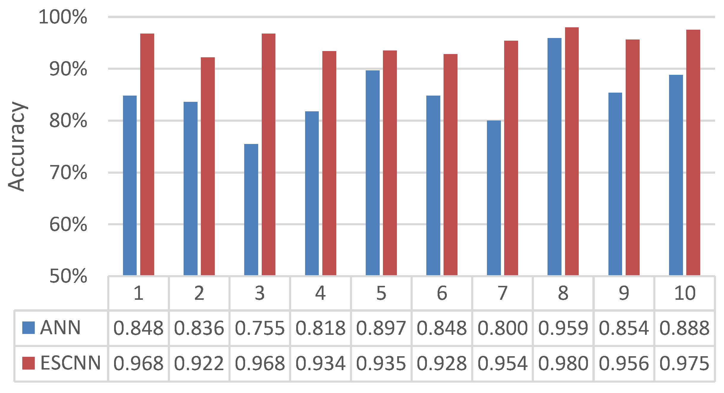
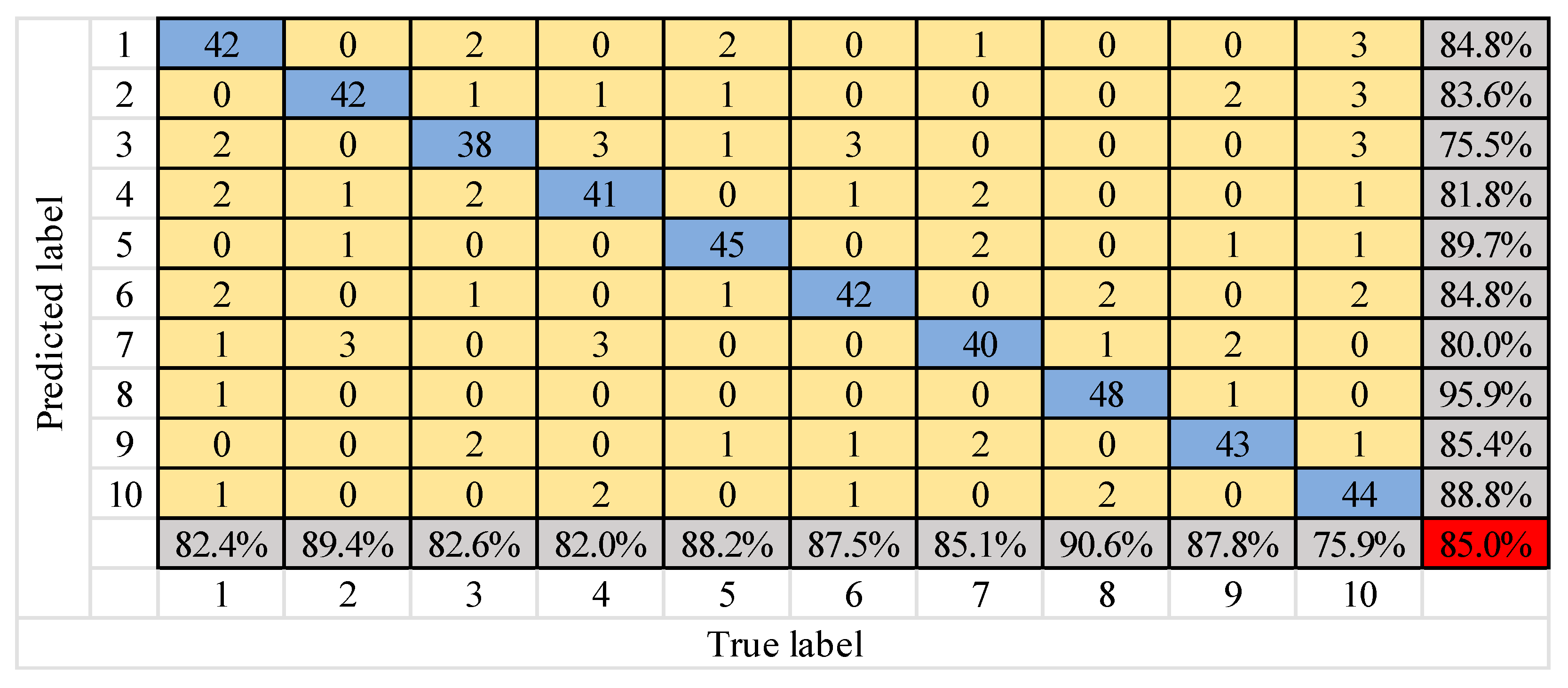
4.3. Performance Analysis

To verify the good recognition rate of ASCNN for the vibration time-frequency diagram of different fault states of gears, we compared the diagnosis results of ASCNN with those of common fast Fourier transform(FFT)–support vector machine (SVM) and FFT–multilayer perceptron (MLP) models [25,26]. The results are as follows (1–10 in the figure represents the fault label, which is consistent with the label of Table 1).
Figure 11 shows that the diagnostic rate of the FFT–SVM model fluctuates between 60% and 76%, which is generally low. The diagnostic rate of the FFT–MLP model fluctuates between 78% and 87%, which is nearly 18 percentage points higher than that of FFT–SVM. The diagnostic rate of ASCNN model was further improved, and even reached 98.2% at 900 r/min. As mentioned, confusion matrix is a standard format to express accuracy evaluation in the form of a matrix of n rows and n columns. Each column represents a prediction category, and each row represents a real category of data. The column is a visual tool that shows the effectiveness of the classification algorithm. The confusion matrix of the diagnosis results of the three models is shown in Figure 12, Figure 13 and Figure 14.
Figure 12, Figure 13 and Figure 14 shows that the number of test samples that can be correctly identified by the FFT–SVM model is up to 38 in the fifth type of fault, and the lowest is 30 in the first type of fault. The overall correct accuracy of the sample is 68.3%. The number of test samples that can be correctly identified by the FFT–MLP model is up to 44 in the tenth type of fault, and the lowest is 39 in the first type of fault. The overall correct accuracy of the sample is 82.9%. The number of test samples that can be correctly identified by the ASCNN model is up to 49 of the sixth, seventh and eighth types of faults, and the lowest is 47 of the second, third and fourth types of faults. The overall correct accuracy of the sample is 95.9% and the error rate is 4.1%, which is the highest overall recognition rate among the three models. Therefore, the ASCNN model is effective for gear fault diagnosis.

5. Diagnostic Performance Analysis of ESCNN

5.1. Data Preparation

The sound signals required for this section are derived from the microphones on the array shelf. According to the setting of Table 1. A total of 10 kinds of gearbox running states are available, and the sampling frequency is 16 KHz. The original audio signal for each fault condition has a duration of 60 s. The research on speech recognition, sound field classification and environmental sound classification shows that the 1–2 s sound segment already contains enough information for feature analysis and classification [27]. Inspired by this, we cut the 60 s original audio into fixed 1 s sound clips. The sliding window was set to 1024 and the moving step to 50%. An audio sample containing approximately 16,000 data points was obtained by segmenting the original audio. Through this method, 200 samples were extracted for each fault state to be used in the ESCNN model training and testing. In the ESCNN model, the steps of feature extraction are delivered to convolutional layers 1 and 2 without manual intervention. We selected four states with a motor speed of 1800 r/min: normal, worn, broken and pitting. The time domain waveform and spectrum for each operating state were analyzed, as shown in Figure 15.
As shown in Figure 15, the time domain map of gear sound signal changes with the gear state. The amplitude of the normal state is the largest and the wear state is the smallest. The spectrogram shows that the amplitude and distribution of the sound signals of different fault types are also inconsistent. The four states have different levels of resonance peaks in the low-frequency band. Three resonance peaks in the normal state exist, two in the wear state, two in the broken state and three in the pitting state, indicating that the sound signal can reflect the fault state of the gear.

5.2. Parameter Settings

The original audio signal of the 10 states of the gear is directly sent to the ESCNN model for fault identification. The model parameters are selected in the same way as the ASCNN model. The three parameters of iteration, learning rate and batch size are still selected in the analysis of the recognition accuracy. The specific process is the same as that of the ASCNN model and is not described here. According to the experimental results, the iteration rate is set to 50, the learning rate to 0.005 and the batch size to 10 in the ESCNN model.

5.3. Performance Analysis

The main advantage of the ESCNN model is that the signal is processed in an end-to-end manner, avoiding the difference in model accuracy caused by manual extraction of features. To verify that ESCNN has a good recognition rate for the audio signal of gear failure, we compared it with the conventional manual feature extraction method, taking reference [28] as an example. Wavelet transform is used to transform data from time domain to frequency domain, and statistical features are extracted and sent to the artificial neural network (ANN) classifier for training. The results are shown in Figure 16.
Figure 16 shows that the diagnostic rate of the ANN model fluctuates between 75.5% and 95.9%, and the amplitude is large, which eventually falls into local optimum. The diagnostic rate of the ESCNN model fluctuates between 92.2% and 98%, which is higher, gentler and more stable than that of the ANN model. The diagnostic results of the two models are shown in Figure 17 and Figure 18.
Figure 17 and Figure 18 show that the number of test samples that can be correctly identified by the ANN model is up to 48 in the eighth type of fault, and the lowest is 38 in the third type of fault. The overall correct accuracy of the sample is 85%. The highest accuracy of ANN is 95.9%, and the minimum is only 75.5%. The gap between them is extremely large, which obviously falls into the local optimum. The number of test samples that can be correctly identified by the ESCNN model is up to 49 in the eighth and tenth types of fault, and the lowest is 46 in the second and sixth types of fault. The overall correct accuracy of the sample is 95.2% and the error rate is 4.8%, which is nearly 10 percentage points higher than that of ANN. In the ESCNN model, the accuracy of the eighth type of fault is the highest, and that of the second type of fault is the lowest, which is consistent with the result of the ASCNN model. Therefore, the ESCNN model is effective for gear fault diagnosis.

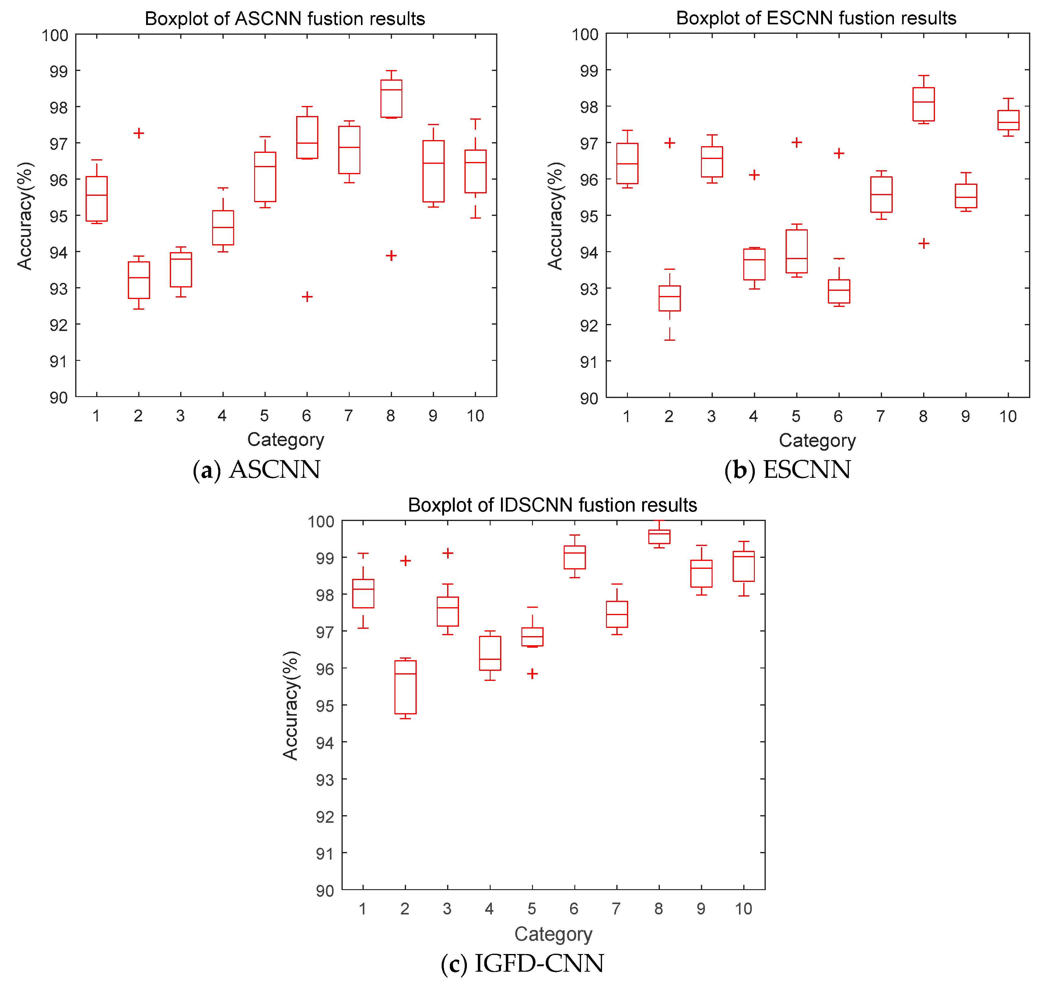
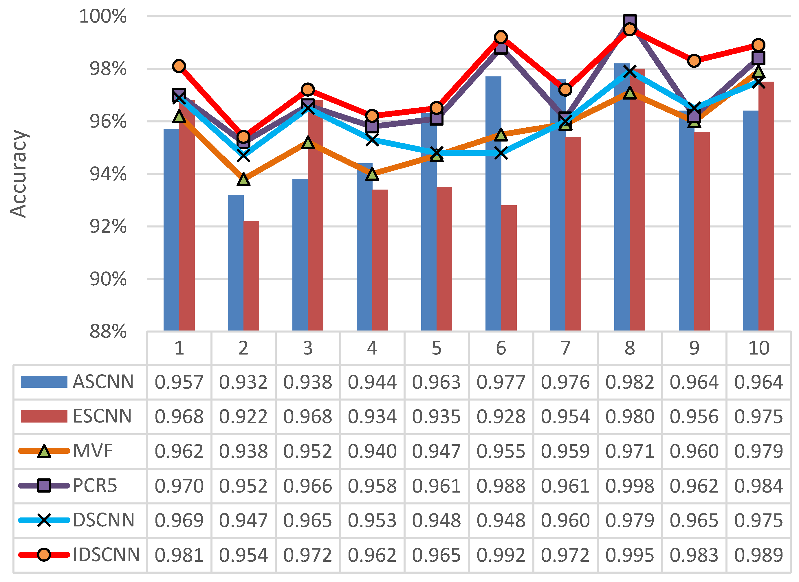
6. Diagnostic Performance Analysis of IGFD-CNN

The sum of the output probabilities of the single source model at the SoftMax layer was exactly 1, which satisfied the requirement that the sum of the basic probability assignments (BPA) of the evidence theory was 1. Therefore, the 10 operating states of the gearbox were used as the identification framework for evidence theory. The output of ASCNN was used as the first evidence (m1), and the output of ESCNN was used as the second evidence (m2). The results of the two models were further determined by IDS theory to obtain an accurate fault identification of the gearbox. To validate the proposed IGFD-CNN model, we compared the diagnostic results with ASCNN and ESCNN. To reduce the impact of randomness and chance on the results, we ran each model 10 times each. The precision of each run was recorded and drawn as a box diagram, as presented in Figure 19.
Figure 19 shows the highest diagnostic rate of ASCNN is the eighth type of fault, and the lowest is the second type. Each of them has an abnormal point. The sixth type of fault also has an abnormal point. The overall performance of the model is dispersed between 93% and 98%. The box length of each type of fault is relatively long, which shows that the 10 diagnosis results are discretely distributed. Except for the sixth category, the median lines of the other nine types of box graphs are on the upper side, tending to the maximum of each category. The highest diagnostic rate of ESCNN is the eighth type of fault and the lowest is the second type. The outliers appear in the second, fourth, fifth, sixth, and eighth types of faults. The diagnosis rate of these five types of faults varies from high to low in the entire ESCNN. The overall performance of the model is dispersed between 92% and 98%, which is low and scattered. Compared with ASCNN, the box length of each type of fault is shorter, which indicates that the 10 diagnosis results have convergence. Although the median line of the fifth type of fault is lower, the other nine types of fault are in the middle trend, showing a stable state. The highest diagnostic rate of IGFD-CNN is the eighth type of fault and the lowest is the second type, which is consistent with the model of ASCNN and ESCNN, indicating that the three models provide consistent conclusions for the fault categories of the highest and lowest diagnostic rates. The diagnosis rate of the eighth type of fault reached 100%, and the abnormal value appeared in the second, third and fifth types of faults, which is close to the box. The overall performance of the model was dispersed between 95% and 99%, which is improved and concentrated compared with the ASCNN and ESCNN. The box of the second type of fault is longer, that of the other nine types is shorter, and their median line is on the upper side, indicating that the 10 diagnosis results are well converged and concentrated. Compared with the three models, the IGFD-CNN model has the shortest box length and small floating range for each type of fault except the second type. Therefore, IGFD-CNN model is more effective than ASCNN and ESCNN.
To further validate the IGFD-CNN model, we compared other fusion methods, such as median voting fusion [29] (MVF), proportional conflict allocation rule 5 [30] (PCR5), and traditional evidence theory (DSCNN). Similarly, to reduce the error, we ran each model 10 times, and the average of 10 experimental results was taken as the final result of data fusion, as shown in Figure 20.
Figure 20 shows that single and multiple sources produce different diagnostic results. The accuracy of fault identification is as low as 92% and as high as 98%, with large error and wide fluctuation range because of the influence of single sensor accuracy, installation position, environment and other factors, which cannot accurately and comprehensively reflect the health state of gear. The combination of multiple signal sources at multiple levels is necessary to obtain the interpretation and description of the consistency of the tested object. Comparing the results of four fusion methods, we find that the IGFD-CNN model has the highest average fault recognition rate (97.7%). The PCR5 fusion rule has the second highest (97%), and DSCNN, which is the traditional evidence theory fusion method, is the third (96.1%). The MVF fusion method is the lowest (95.6%). The improved fusion algorithm in this study uses the weight of evidence and sensor to modify the BPA of evidence, and selects the fusion rules for the modified evidence according to the relationship between the threshold and conflict factors. The evidence with high confidence level increases continuously. The evidence with low confidence level decreases continuously, and the ideal diagnosis rate is obtained. The PCR5 fusion rule is mainly applicable to the case of complete conflict of evidence. The evidence in this section is not completely in conflict and cannot show its advantages. The BPA of evidence is allocated according to the original confidence level, which is relatively conservative. Thus, the PCR5 is the second highest diagnostic rate. The diagnosis rate of the traditional DS fusion method is higher than that of a single signal, which fully embodies the advantages of fusion. The principle of the median voting algorithm is “voting, majority passing”. This algorithm is a simple and fast method without complex operation, which can be completed in the shortest time, but the diagnostic rate is the lowest of the four methods.

7. Conclusions

In this study, a sound signal was added to the vibration signal to form multi-source information, which overcame the limitations of the single signal and sensor itself. A diagnosis method of multi-source sensor fusion vibration and sound signals based on IGFD-CNN was proposed. First, a gearbox fault diagnosis platform was built in the semi-anechoic chamber environment to collect vibration and sound signals under different working conditions. Second, the vibration signal is pre-processed into a time-frequency map and sent to the ASCNN model, and the sound signal was directly sliced into the ESCNN model. The respective primary diagnosis was obtained by adjusting the parameters of the model. Finally, the IDS method was used to further integrate the primary diagnosis results of vibration and sound signals. The experimental results showed that 97.7% of the average fault recognition rate was obtained using the model discussed in this paper. Compared with the single signal source, a reliable equipment operation state could be obtained by fusing multi-source signals.

Author Contributions

Funding acquisition, L.Y.; investigation, J.Y. and X.Y.; methodology, J.Y. and X.Y.; supervision, L.Y.; writing—original draft, L.Y. and X.Y.; writing—review and editing, L.Y., X.Y., J.Y. and C.L.; Polish, C.L. All authors have read and agreed to the published version of the manuscript.

Funding

This research was funded by National Natural Science Foundation of China under Grant Nos. 91746116 and 51741101, and Science and Technology Project of Guizhou Province under Grant Nos. QKHJ [2010]2095.

Acknowledgments

We gratefully acknowledge the support of the NVIDIA Corporation with the donation of the Titan X Pascal GPU used for this research.

Conflicts of Interest

The authors declare no conflicts of interest.

References

  1. Yang, J.; Li, S.; Gao, Z.; Wang, Z.; Liu, W. Real-time recognition method for 0.8 cm darning needles and KR22 bearings based on convolution neural networks and data increase. Appl. Sci. 2018, 8, 1857. [Google Scholar] [CrossRef] [Green Version]
  2. Weikang, L.W.J. Diagnosing Rolling Bearing Faults Using Spatial Distribution Features of Sound Field. J. Mech. Eng. 2012, 13, 68–72. [Google Scholar]
  3. Zhao Shutao, W.Y.L.M. Breaker Fault Diagnosis with Sound and Vibration Characteristic Entropy. J. North China Electr. Power Univ. 2016, 43, 20–24. [Google Scholar]
  4. Khazaee, M.; Ahmadi, H.; Omid, M.; Moosavian, A.; Khazaee, M. Classifier fusion of vibration and acoustic signals for fault diagnosis and classification of planetary gears based on Dempster–Shafer evidence theory. Proc. Inst. Mech. Eng. Part E J. Process Mech. Eng. 2014, 228, 21–32. [Google Scholar] [CrossRef]
  5. Moosavian, A.; Khazaee, M.; Najafi, G.; Kettner, M.; Mamat, R. Spark plug fault recognition based on sensor fusion and classifier combination using Dempster–Shafer evidence theory. Appl. Acoust. 2015, 93, 120–129. [Google Scholar] [CrossRef] [Green Version]
  6. Othman, M.S.; Nuawi, M.Z.; Mohamed, R. Vibration and Acoustic Emission Signal Monitoring for Detection of Induction Motor Bearing Fault. Int. J. Eng. Res. Technol. (IJERT) 2015, 4, 924–929. [Google Scholar]
  7. Martínez-García, C.; Astorga-Zaragoza, C.; Puig, V.; Reyes-Reyes, J.; López-Estrada, F. A simple nonlinear observer for state and unknown input estimation: DC motor applications. IEEE Trans. Circuits Syst. II Express Briefs 2019, 4, 710–714. [Google Scholar] [CrossRef]
  8. Yuzukirmizi, M.; Arslan, H. Fault diagnosis of shaft-ball bearing system using one-way analysis of variance. Math. Comput. Appl. 2014, 19, 37–49. [Google Scholar] [CrossRef] [Green Version]
  9. López-Estrada, F.; Rotondo, D.; Valencia-Palomo, G. A Review of Convex Approaches for Control, Observation and Safety of Linear Parameter Varying and Takagi-Sugeno Systems. Processes 2019, 7, 814. [Google Scholar] [CrossRef] [Green Version]
  10. Yang, J.; Li, S.; Wang, Z.; Yang, G. Real-time tiny part defect detection system in manufacturing using deep learning. IEEE Access 2019, 7, 89278–89291. [Google Scholar] [CrossRef]
  11. Yang, G.; Yang, J.; Sheng, W.; Junior, F.; Li, S. Convolutional neural network-based embarrassing situation detection under camera for social robot in smart homes. Sensors 2018, 18, 1530. [Google Scholar] [CrossRef] [PubMed] [Green Version]
  12. Krizhevsky, A.; Sutskever, I.; Hinton, G.E. Imagenet classification with deep convolutional neural networks. In Proceedings of the 25st Neural Information Processing Systems (NIPS 2012), Lake Tahoe, NV, USA, 6–12 December 2012; pp. 1097–1105. [Google Scholar]
  13. Sermanet, P.; Chintala, S.; LeCun, Y. Convolutional neural networks applied to house numbers digit classification. In Proceedings of the 21st International Conference on Pattern Recognition (ICPR2012), Tsukuba, Japan, 11–15 November 2012; IEEE: Piscataway, NJ, USA; pp. 3288–3291. [Google Scholar]
  14. Yang, J.; Yang, G. Modified convolutional neural network based on dropout and the stochastic gradient descent optimizer. Algorithms 2018, 11, 28. [Google Scholar] [CrossRef] [Green Version]
  15. He, K.; Zhang, X.; Ren, S.; Sun, J. Deep residual learning for image recognition. arXiv 2015, arXiv:1512.03385. [Google Scholar]
  16. Aytar, Y.; Vondrick, C.; Torralba, A. Soundnet: Learning sound representations from unlabeled video. arXiv 2016, arXiv:1610.09001. [Google Scholar]
  17. Silver, D.; Huang, A.; Maddison, C.J.; Guez, A.; Sifre, L.; Van Den Driessche, G.; Schrittwieser, J.; Antonoglou, I.; Panneershelvam, V.; Lanctot, M. Mastering the game of Go with deep neural networks and tree search. Nature 2016, 529, 484–489. [Google Scholar] [CrossRef]
  18. Esteva, A.; Kuprel, B.; Novoa, R.A.; Ko, J.; Swetter, S.M.; Blau, H.M.; Thrun, S. Correction: Corrigendum: Dermatologist-level classification of skin cancer with deep neural networks. Nature 2017, 546, 686. [Google Scholar] [CrossRef]
  19. Granda, D.; Aguilar, W.G.; Arcos-Aviles, D.; Sotomayor, D. Broken bar diagnosis for squirrel cage induction motors using frequency analysis based on MCSA and continuous wavelet transform. Math. Comput. Appl. 2017, 22, 30–45. [Google Scholar]
  20. Yao, X.; Li, S.; Yao, Y.; Xie, X. Health monitoring and diagnosis of equipment based on multi-sensor fusion. Int. J. Online Biomed. Eng. (IJOE) 2018, 14, 4–19. [Google Scholar] [CrossRef] [Green Version]
  21. Yao, Y.; Wang, H.; Li, S.; Liu, Z.; Gui, G.; Dan, Y.; Hu, J. End-to-end convolutional neural network model for gear fault diagnosis based on sound signals. Appl. Sci. 2018, 8, 1584. [Google Scholar] [CrossRef] [Green Version]
  22. Yang, Y. Study on Fault Diagnosis System of Worm-gear Reducer Based on Wavelet Analysis. Electron. Sci. Technol. 2016, 29, 65–69. [Google Scholar]
  23. Huang, L.; Wu, C.; Wang, J. Fault pattern recognition of rolling bearing using wavelet package analysis and BP neural network. Electron. Meas. Technol. 2016, 39, 164–168. [Google Scholar]
  24. Cai, G.; Selesnick, W.; Wang, S.; Weiwei, D.; Zhou, Z. Sparsity-enhanced signal decomposition via generalized minimax-concave penalty for gearbox fault diagnosis. J. Sound Vib. 2018, 432, 213–234. [Google Scholar] [CrossRef]
  25. Jia, F.; Lei, Y.; Lin, J.; Zhou, X.; Lu, N. Deep neural networks: A promising tool for fault characteristic mining and intelligent diagnosis of rotating machinery with massive data. Mech. Syst. Signal. Process. 2016, 72, 303–315. [Google Scholar] [CrossRef]
  26. Zhang, W.; Peng, G.; Li, C.; Chen, Y.; Zhang, Z. A new deep learning model for fault diagnosis with good anti-noise and domain adaptation ability on raw vibration signals. Sensors 2017, 17, 425. [Google Scholar] [CrossRef]
  27. Piczak, K.J. ESC: Dataset for environmental sound classification. In Proceedings of the 23rd ACM International Conference on Multimedia, Brisbane, Australia, 26–30 October 2015; pp. 1015–1018. [Google Scholar]
  28. Khazaee, M.; Ahmadi, H.; Omid, M.; Banakar, A.; Moosavian, A. Feature-level fusion based on wavelet transform and artificial neural network for fault diagnosis of planetary gearbox using acoustic and vibration signals. Insight Non-Destruct. Test. Cond. Monit. 2013, 55, 323–330. [Google Scholar] [CrossRef]
  29. Zhou, G.; Ge, S.; Yang, L. Fault diagnosis method for nuclear power plants based on neural networks and voting fusion. Energy Sci. Technol. 2010, 44, 367–372. [Google Scholar]
  30. Zhai, X.; Hu, J.; Xie, S.; Liu, J.; Li, Q. Diagnosis of aero-engine with early vibration fault symptom using DSmT. J. Aerosp. Power 2012, 27, 301–306. [Google Scholar]
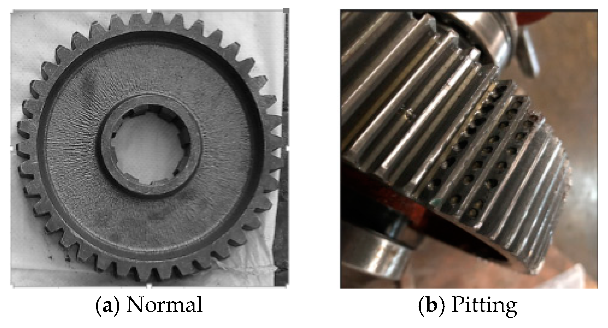
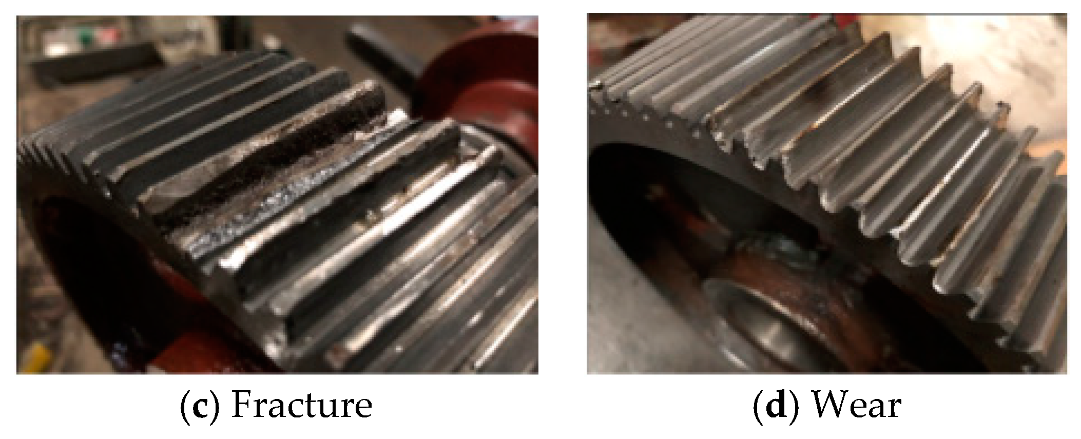
Figure 1. Block diagram of a convolutional neural network to implement gearbox fault diagnosis (IGFD-CNN) model based on vibration and acoustic signals.
Information 11 00266 g001
Figure 2. Gearbox fault experimental platform.
Information 11 00266 g002
Figure 3. Different fault patterns of gears.
Information 11 00266 g003aInformation 11 00266 g003b
Figure 4. Time domain, spectrum and time–frequency diagrams of normal gears.
Information 11 00266 g004
Figure 5. Time domain, spectrum and time–frequency diagrams of worn gears.
Information 11 00266 g005
Figure 6. Time domain, spectrum and time–frequency diagrams of broken gears.
Information 11 00266 g006
Figure 7. Time domain, spectrum and time–frequency diagrams of pitting gears.
Information 11 00266 g007
Figure 8. Fault recognition accuracy curves with iteration.
Information 11 00266 g008
Figure 9. Fault recognition accuracy curve with different learning rates.
Information 11 00266 g009
Figure 10. Fault recognition accuracy curve with different batch sizes.
Information 11 00266 g010
Figure 11. Comparison of diagnostic effects of different models on gearbox failure.
Information 11 00266 g011
Figure 12. Confusion matrix of fast Fourier transform (FFT)–support vector machine (SVM) model diagnosis results.
Information 11 00266 g012
Figure 13. Confusion matrix of FFT–multilayer perceptron (MLP) model diagnosis results.
Information 11 00266 g013
Figure 14. Confusion matrix of ASCNN model diagnosis results.
Information 11 00266 g014
Figure 15. Time domain and spectrogram of gear sound signal.
Information 11 00266 g015
Figure 16. Comparison of diagnostic effects of artificial neural network (ANN) and ESCNN models on gearbox failure.
Information 11 00266 g016
Figure 17. Confusion matrix of ANN model diagnosis results.
Information 11 00266 g017
Figure 18. Confusion matrix of ESCNN model diagnosis results.
Information 11 00266 g018
Figure 19. Box diagrams of fusion results of different models.
Information 11 00266 g019
Figure 20. Comparison of diagnostic results for single and multiple sources.
Information 11 00266 g020
Table 1. Description of gear datasets.
NormalPittingFractureWear
Category Labels12345678910Total
Speed (r/m)900900180027009001800270090018002700
VibrationTrain1501501501501501501501501501502000
Test50505050505050505050
AcousticalTrain1501501501501501501501501501502000
Test50505050505050505050
FusionTrain3003003003003003003003003003004000
Test100100100100100100100100100100

