Article

Comparative Analysis among Discrete Fourier Transform, K-Means and Artificial Neural Networks Image Processing Techniques Oriented on Quality Control of Assembled Tires

by
Alessandro Massaro
*,
Giovanni Dipierro
,
Emanuele Cannella
and
Angelo Maurizio Galiano
Dyrecta Lab, Research Institute, Via Vescovo Simplicio 45, 70014 Conversano (BA), Italy
*
Author to whom correspondence should be addressed.
Information 2020, 11(5), 257; https://doi.org/10.3390/info11050257
Submission received: 21 April 2020 / Revised: 6 May 2020 / Accepted: 7 May 2020 / Published: 8 May 2020
(This article belongs to the Section Information Applications)

Abstract

:
The present paper discusses a comparative application of image processing techniques, i.e., Discrete Fourier Transform, K-Means clustering and Artificial Neural Network, for the detection of defects in the industrial context of assembled tires. The used Artificial Neural Network technique is based on Long Short-Term Memory and Fully Connected neural networks. The investigations focus on the monitoring and quality control of defects, which may appear on the external surface of tires after being assembled. Those defects are caused from tires which are not properly assembled to their respective metallic wheel rim, generating deformations and scrapes which are not desired. The proposed image processing techniques are applied on raw high-resolution images, which are acquired by in-line imaging and optical instruments. All the described techniques, i.e., Discrete Fourier Transform, K-Means clustering and Long Short-Term Memory, were able to determine defected and acceptable external tire surfaces. The proposed research is taken in the context of an industrial project which focuses on the development of automated quality control and monitoring methodologies, within the field of Industry 4.0 facilities. The image processing techniques are thus meant to be adopted into production processes, giving a strong support to the in-line quality control phase.

1. Introduction

Within the automotive field, the assembling process between the tire and its corresponding wheel rim represents an industrial activity which requires highly engineered technologies. Such technologies are continuously improving to enhance the efficiency in production. This process is usually required by the main automotive companies, which may assign the activity to third-party industries, which have to ensure a high-quality standard. To achieve the highest results, it is possible to take advantage of the most modern analytical approaches. In particular, the Lean Methodology [1,2,3] is used in case of activities including the evaluation of defects. Starting from the analysis of the tire-wheel rim assembling process [4], image processing techniques can provide important insights about possible defects, visible as patterns, which may occur on the external surface of the tire [5]. Those analyses are combined with the Ethernet network [6], as enabling Industry 4.0 technology. Many companies are therefore implementing the combination of Ethernet systems and Internet of Things (IoT) [7] to enhance the traceability in production [8], collecting significant improvements. A comprehensive scenario of the production processes may be shown by using either fishbone diagrams or a roof-shaped L-matrix diagrams, which immediately show information about defects [9] and enhance the production according to the ISO 9001:2015 quality standards. Some authors [10] have adopted IoT techniques to identify tire defects. Different approaches for the detection and classification of defects have been recently investigated in various fields, including generative adversarial networks [11,12], variational autoencoders [13,14,15,16,17] and iterative energy-based projection [18]. The previously mentioned approaches enable unsupervised anomaly detection by leveraging the ability of these methods to detect anomalies by comparing test examples with images reconstructed by the models. Important approaches for the detection of tire defects consist of the image processing algorithms [19,20]. The angle of view is a critical aspect concerning non-destructive image inspection [20].
The main content of this paper focuses on the analysis of assembled tire images which are in-line acquired to support the quality control phase. Specifically, image vision techniques are applied to analyse the presence of defects within the assembled tires in terms of scratch and folded tire rubber which may be unsafe for the assembled products. K-Means, Discrete Fourier Transform (DFT) and Long Short-Term Memory-Fully Connected (LSTM-FC) neural networks (as a method in the field of Artificial Neural Network—ANN) techniques are applied and compared in order to identify the presence of defects within the components. Following the state-of-the-art mentioned in this paper, different tools and combined approaches are investigated for future development and improvements of an industrial platform designed for in-line monitoring. This platform will be enhanced from the image processing techniques hereby described, to provide defect recognition and classification. The proposed work is therefore exploring the capability of those techniques, i.e., K-Means, DFT and LSTM-FC, to correctly detect defects and infer which is the most effective tool, following Industry 4.0 principles.

2. Materials and Methods: Measurement Setup

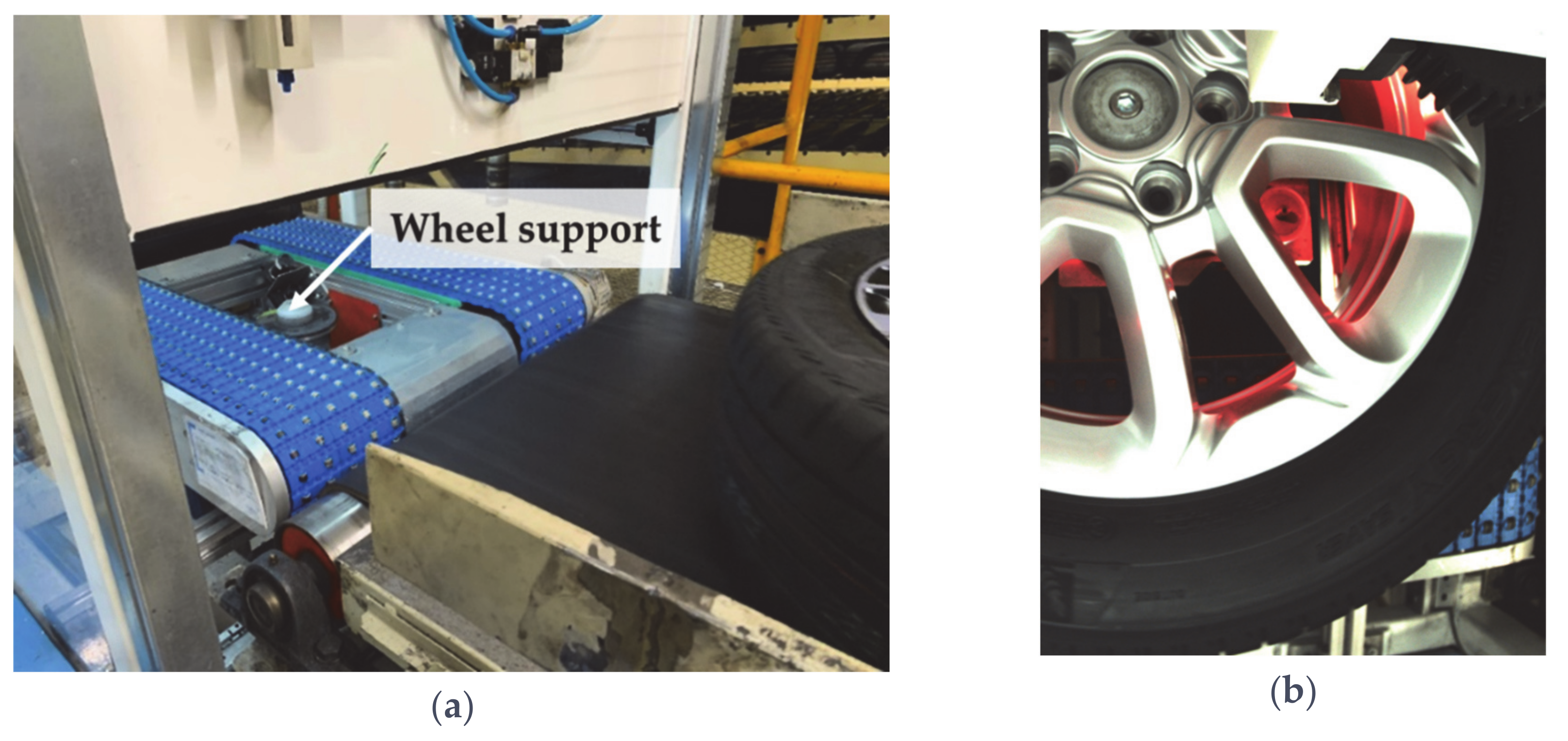
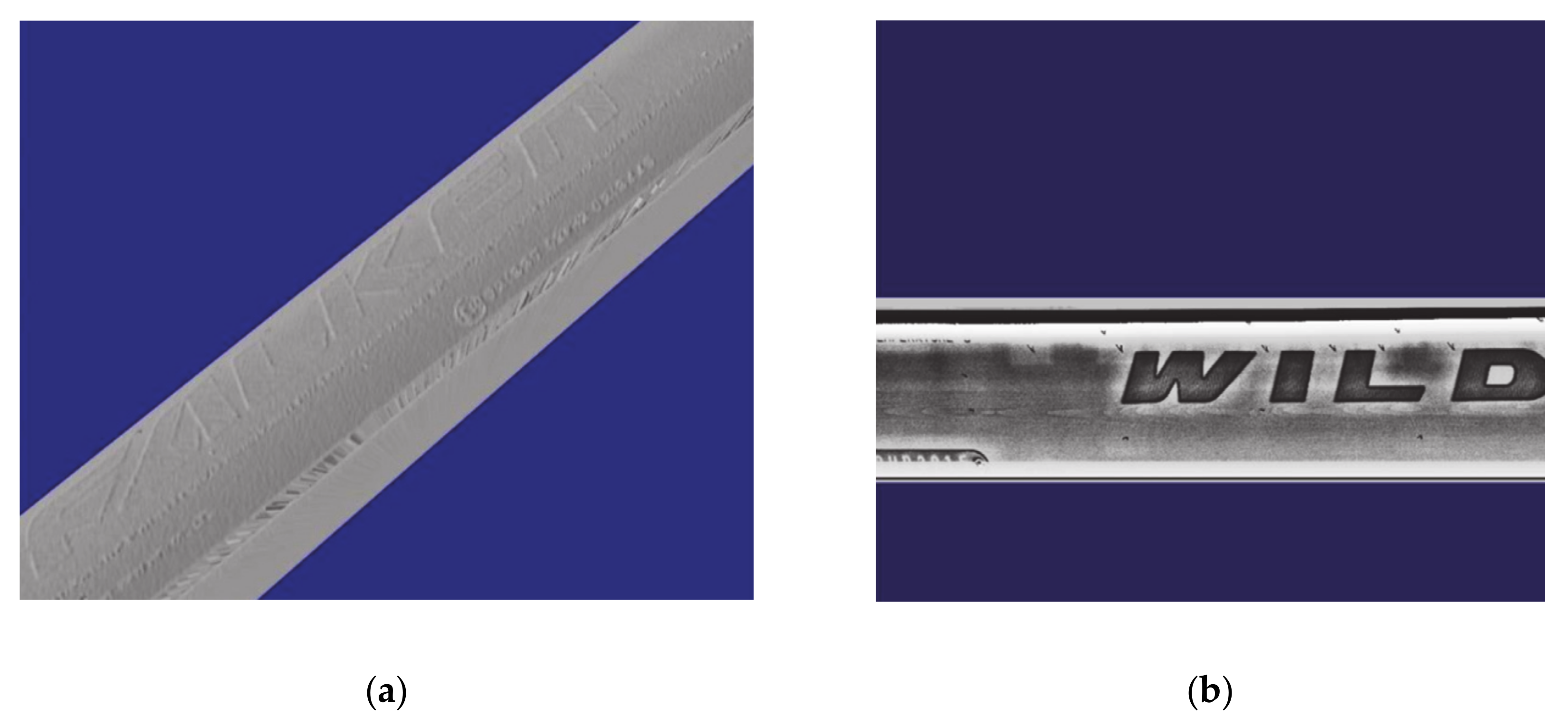
The industrial system (Coditech) used for data acquisition of the tire-wheel assembly is mainly made of a laser profilometer and a detector, as shown in Figure 1. The profilometer acquires 1280 points per profile, with axes X, Z resolutions varying within ranges 0.019–0.060 mm and 0.150–0.300 mm, respectively. The laser class is 3R. The assembled wheel is rotated by 360° over the support shown in Figure 2a, while the laser is fixed on the top of the apparatus to scan the lateral profile of the wheel, Figure 2b. The captured profile is therefore processed by the software, which produces the 3D reconstruction of the tire profile. The 3D reconstruction is converted to a 2D image as shown in Figure 3, in order to decrease the computing time which is required for the whole analysis. This process is made by interpolating the pictures obtained by slicing the z-axis of the profile. The 2D pictures are saved as TIFF compressed images of the tire sidewall, with a file size of about 1200 kb. The total processing time lasts about 12 s. This time is fundamental to comply with the requirements given from the company, which has to ensure a fast quality control, which can be comparable to the cycle time required for the assembling of a complete set, i.e., four tires. The 2D pictures represent the input data which are analysed by the image processing techniques proposed in this paper.
The ImageJ Surface Plot 3D library (in this case, the third dimension is given from the colour intensity axis), is used as an image manipulation tool which enables the possibility to highlight the presence of possible undesired defects and morphological information of the tire. This tool has been described in literature about the morphology investigations of micro and nano-structured surfaces [21], where the 3D reconstruction has provided many details about the nano-scale morphology. In this application, the image processing approach is followed to highlight the presence possible undesired tire stresses generated by an incorrect assembly process. The tire-wheel rim assembly produces large deformations and displacements on the tire, due to the pressure which is required to carry out the assembly. Stresses and deformations are mostly reflected on the elastic properties of the tire, due to the high stiffness of the wheel [22]. Unusual deformations and stresses, caused by possible incorrect procedures, have to be controlled in order to guarantee the correct functionality of the product. For this purpose, the reconstruction is processed with isolines approach in order to trace the defect pattern. The library “3D Surface Plot” by ImageJ is adopted for the purpose. A I7-9700 computer processor (M.2 512 GB PCIe NVMe, Intel H310) with a CUDA Cores 256 board (GPU Memory 2 GB GDDR5) is adopted for data processing. This processor is employed to run the ImageJ software, DFT, K-Means and ANN. The defects can therefore be pre-classified and stored into a database system as performed in [23,24].
As a summary, the following flowchart in Figure 4 shows the detailed steps which are followed in this research article. The K-Means and DFT techniques followed a similar path, as highlighted from the flowchart.
Before showing the obtained results, the next Section 3 will theoretically discuss the above-mentioned techniques.

3. Defect Detection Techniques

When considering the assembling process of tires, their inspection represents a fundamental task made to ensure the product quality and investigate the presence of defects [25]. The quality control has to comply with several requirements, e.g., flexibility, promptness and accuracy, due to the rapid transition towards Industry 4.0.
As mentioned in the previous section, the detection and morphology classification of surface defects can be performed by image processing techniques, i.e., Discrete Fourier Transform (DFT), K-Means Clustering and Artificial Neural Networks. These techniques are hereby investigated in terms of computational time and accuracy. The aim is to evaluate the most effective method for defect detection.

3.1. K-Means Clustering

The K-Means technique has been largely described in literature [26,27,28], e.g., when monitoring photovoltaic panels [29], thus suggesting its application in other fields which involve defect evaluations. The algorithm used by K-Means is based on the segmentation of the image into different non-overlapping areas, which are characterised by the same properties (e.g., shape, intensity, scale).
Pixels which have the same intensity (grey scale level) are classified into clusters. The K-Value, which is related to the number of clusters, is chosen to be representative of the spatial features of the image to be analysed: a high number of clusters may easily detect an anomalous area. However, a too large number of clusters may negatively influence the defect evaluation process [30]. For this purpose, it is important to set the correct trade-off value of clusters in order to optimize the detection capabilities and computational cost. The ImageJ library is suitable to carry out the K-Means image processing [31].

3.2. Discrete Fourier Transform

DFT is one of the most used techniques to characterize the spatial morphology of an image and infer the presence of image patterns in the spatial domain [32,33,34,35]. The DFT spectra is found to be used in other literature cases, in the context of diagnostic tools for quality control. For example, Fanti and Basso [36] investigated the occurrence of mechanical defects in the case of gear pumps. By analysing the discharge pressure, the signal is processed via Fourier Transform to detect the presence and position of defects. Spectra obtained from defected gears present additional peaks which differed from the non-defected case.
For our purposes, the detection algorithm is based on the analysis of the amplitude spectrum of the Fourier transform, which provides the amplitude of each component of the image in the spatial frequency domain. A defect can be easily detected and spatially characterized as a variation of the amplitude of the Fourier spectrum with respect to the one obtained by analysing a homogeneous image region.
The analysis is performed by using the DFT ImageJ library. The frequency spectrum is shown on a logarithmic scale by considering the results of the Fourier domain origin at volume-centre. The 3D image processing of the DFT frequency spectrum is obtained by using the 3D Surface Plot library. Results are stored into a database [23,24].

3.3. Neural Networks

Neural network techniques have shown state-of-the-art performance in many computer vision tasks [37]. Neural networks usually adopted in computer vision (based on Convolutional Neural Networks, CNN) requires a large number of labelled examples to train and test the neural network. In our case study, the insufficient number of images that were actually collected do not allow to build a neural network based on feature extraction on images. Moreover, since tire sidewalls are characterized by different types of features (e.g., brand, size, shape, texture), the labelling of defects may require manual data annotation by experts who have specialized skills. An alternative approach is based on the use of Long Short-Term Memory (LSTM) method, a variant of recurrent neural networks. The method is based on the patterns learning in timeseries data, which, in our case study, is represented by a single tire sidewall. Importantly, this method assumes that each image can be considered as a unique train dataset for a specific neural network, since it is based on splitting a single image into a collection of sub images that will be used as training dataset. On the other hand, since a neural network is built on each single image, this method might be limited in terms of practical use. The time dimension, according to our approach, is therefore given by the horizontal dimension of the image. Wang et al. [38] showed a defect recognition application based on the FCN approach, which was applied to the tire treads. They concluded that the method may be suitable to be adopted for different types of defect.
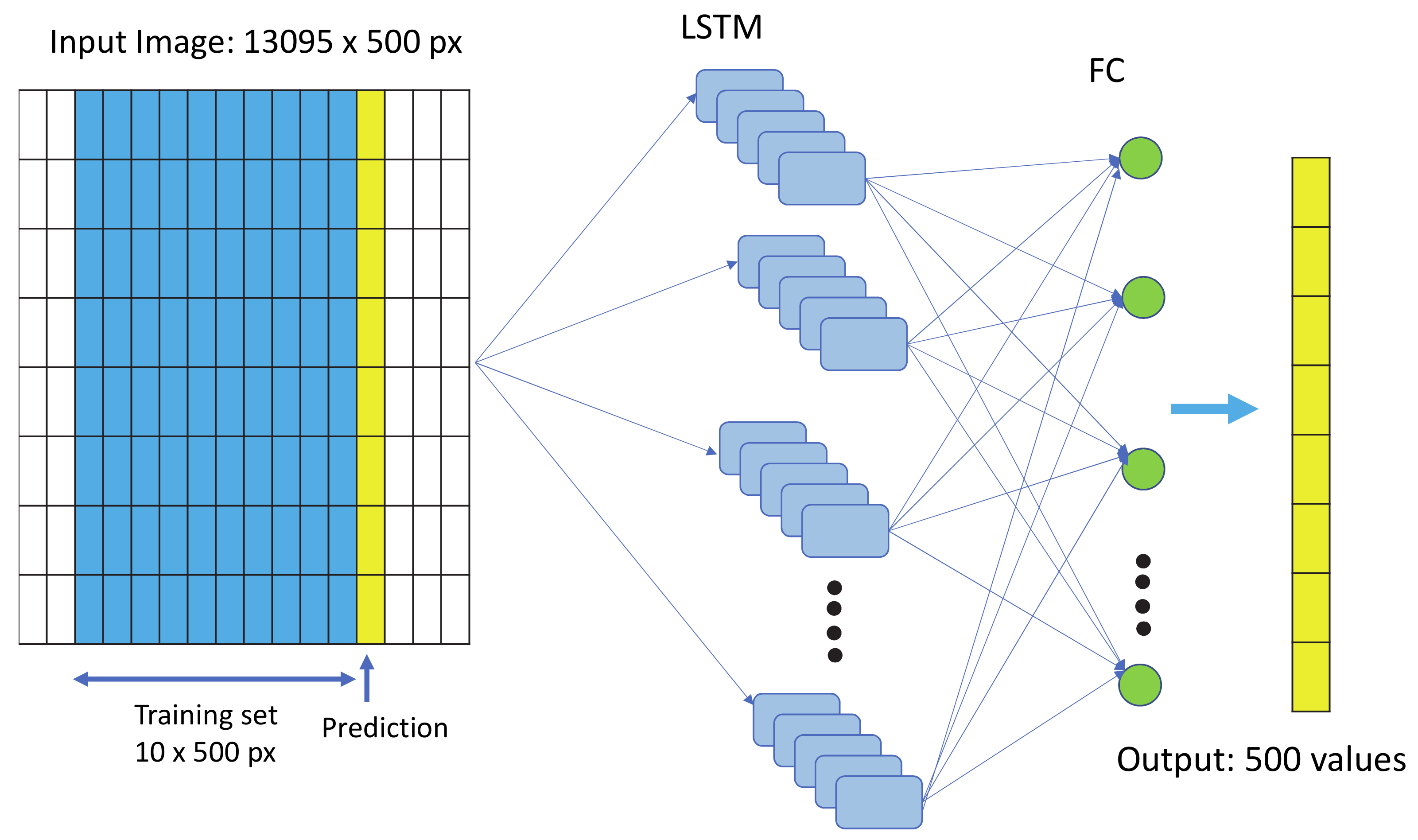
We split the image of the tire sidewall (with resolution 13,095 × 500 pixels) along the horizontal dimension (length of tire sidewall) into a number of sub images with size 10 × 500, each of which is shifted from the previous one by one pixel along the horizontal dimension of the image. Moreover, for each of the latter images we consider the adjacent slice of image with dimension 1 × 500 as the image that the neural network will predict. All the dataset is therefore made by 13,084 couple of images representing the image time sequence over which the neural network will be trained (see the left panel of Figure 5). The images are not resized in order to avoid losing resolution. We build up a linear stack of neural network layers made by long-short time memory and fully-connected neural networks in order to train a model able to recognize all the main morphological features of the single tire and the spatial (time) distribution of the feature along the tire. In detail, we stack two LSTM layers on top of each other and three fully-connected neural networks, with the output sequence of one layer forming the input sequence for the next. Figure 5 shows the structure of the stack of LSTM and FC layers proposed in this paper. While the LSTM layers are devoted to infer the recurrent features of the tire sidewall taking into account the long-range dependencies, the FC layers capture the spatial dependencies between adjacent pixel layers. The neural network is trained for 25 epochs using a learning rate of 0.0002. The mean squared error function is adopted as loss function to measure the performance of the network. As previously described, a defect can be classified as a non-recurrent feature in a tire sidewall that does not belong to any features identified by the neural network.
In order to detect the defects, we use the model over the same collection of images and compute, for each sub image, the mean squared error between the real and predicted model. This approach allows us to infer the regions where the model fail to predict the next slices of pixel taking into account the recurrent morphological features thanks to the use of the LSTM architecture. In other word, we use the memory capabilities of the LSTM to infer which slice of pixel shows a defect since its spatial features are not consistent with the features of the whole tire.
Using this approach, a defect can be automatically identified as a region of the tire where the mean squared error is maximized. To this aim, the algorithm includes a routine aimed at finding the maxima of the mean squared error function computed on each predicted image. For simplicity, a defect is identified as the region where the maximum of the mean squared error function falls outside one standard deviation from the mean of the function. It is worth remarking that the proposed neural network enables unsupervised learning, avoiding the need for labelled training data.

4. Results

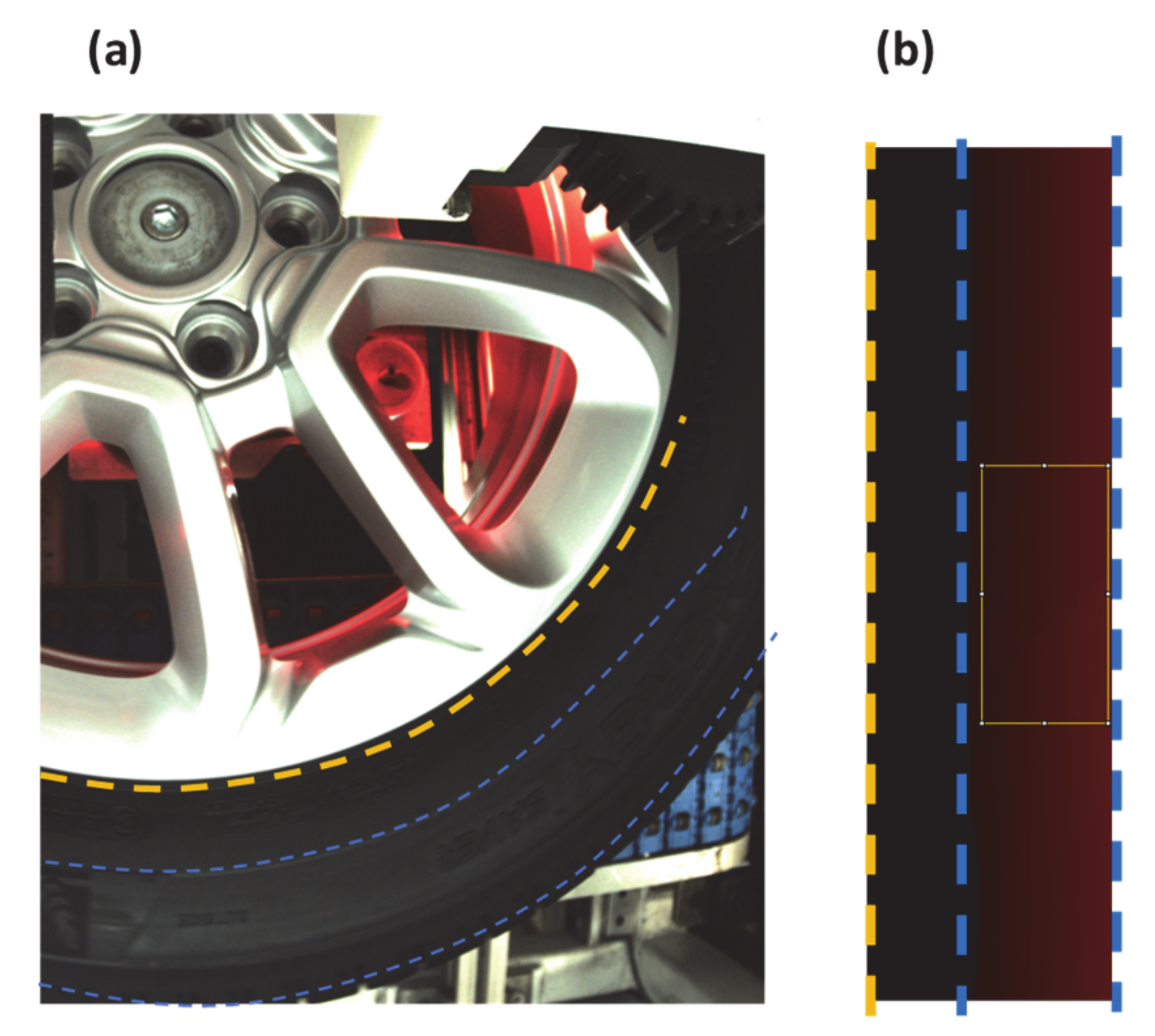
The raw images are collected by means of the inline setup shown in Figure 1, capturing the frontal view of the tire as shown in Figure 6a. As described in Section 2, the image is linearized and cropped around the edges in order to show the tire sidewall (Figure 6b).
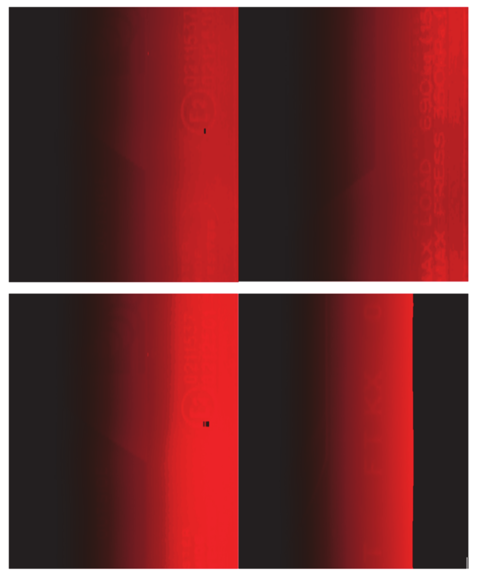
The comparative analysis is carried out on a large number of images (around 100 images), showing the same performance of defect detection of the three different algorithms. For the sake of conciseness, we limit the presentation of results over those related on a representative dataset. This dataset is made of images of sidewalls of four tires with different brand and surface texture, as shown in Figure 7.

4.1. K-Means

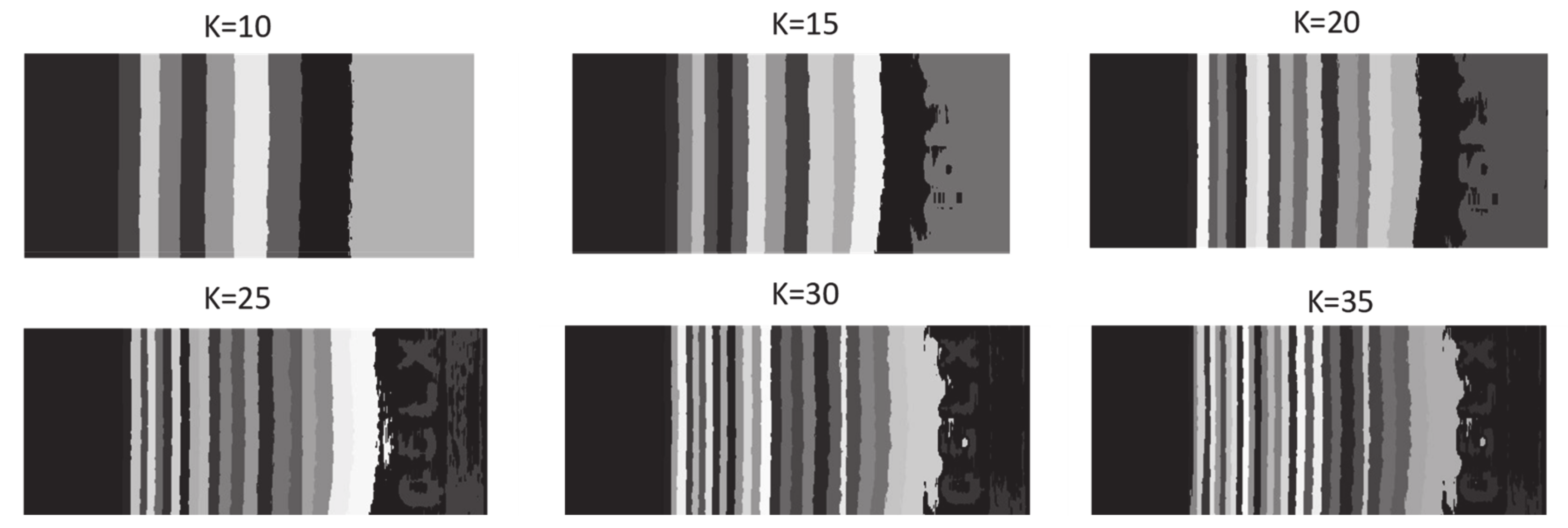
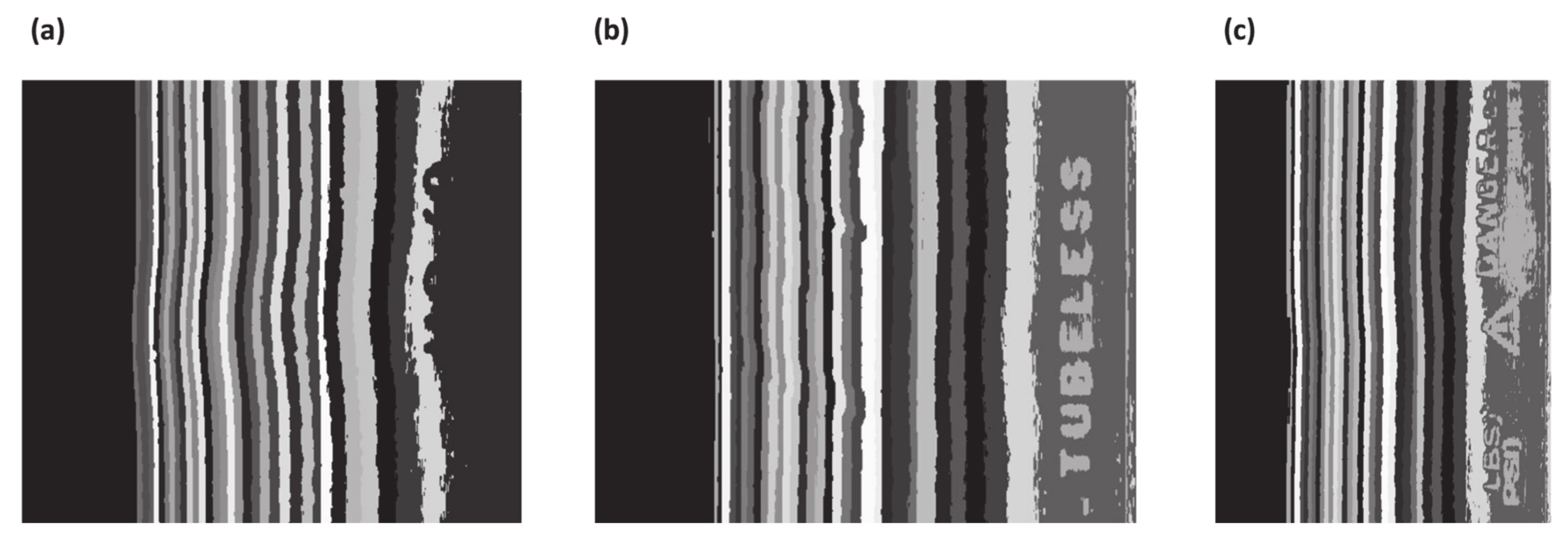
Figure 8 shows the results of the application of the K-Means algorithm with different number of clusters on a homogeneous region of one of the images of the dataset. By setting a large number of clusters (K-Value) it can be noticed that the number of adjacent pixels characterized by the same intensity decreases. The parallel line pattern describes a homogeneous tire region. We observe that for a K-Value larger than 20, the text code of the tire is even visible. By analysing the capabilities of the algorithm in terms of accuracy and practical use, we find that K = 30 is the best trade-off between resolution and computational cost (see Appendix A). The choice of the K-Value can be further optimized by enhancing the hardware technology used for processing and improving the available number of rotary encoders. Figure 9 illustrates an example of a defect classification obtained by using the K-Means processing approach on different regions of the image, using a value of K = 35. The defect classification of Figure 9 is performed by analysing the difference between a homogeneous region with respect to an inhomogeneous one. The observed defects are mainly represented as distributed stresses (Figure 9a), local defects (see Figure 9b) that can be detected as local deviations of contour lines from the vertical, and partially distributed local defects (see Figure 9c) where the distributed stresses are observed in a partial region.
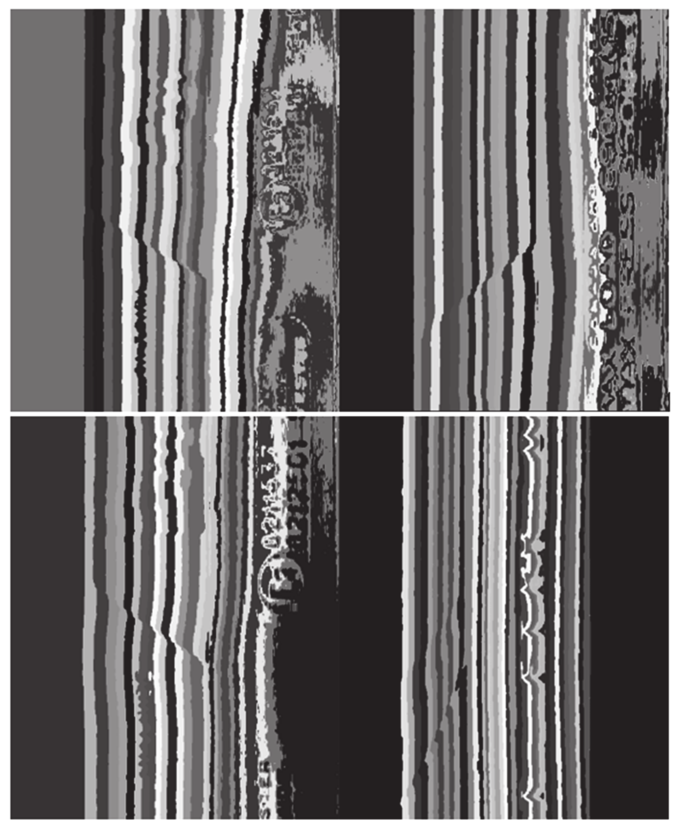
Figure 10 shows all the four images in the dataset after being processed by the K-Means algorithm. For most of the images, the K-Means algorithm enhances regions of defects, showing spatial changes in the distribution of image intensity.
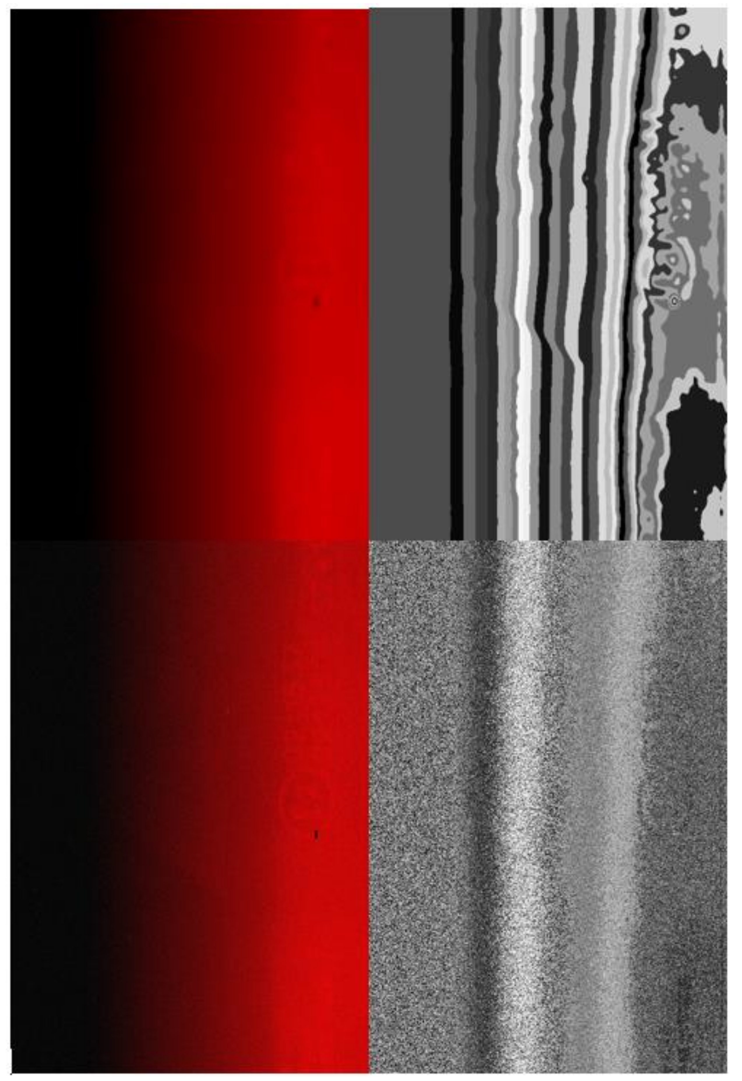
In order to investigate the practical use of the algorithm, the method is applied on noisy images of a tire sidewall. It might occur that external effects acting on the image acquisition system or the low resolution of images might affect the performance of defect detection algorithms. In order to mimic such effects, Gaussian blurring and white noise with a dispersion factor of 8 pixels are used to generate noisy images starting from one representative image of the dataset. In Figure 11 is shown the pre-processed images where the two type of noise are applied (left) and the related K-Means images (right). It can be noticed that, while a decrease of image resolution of a factor 8 might worsen the detection performance of defects, external effects producing small scale noise on the captured image might compromise the detection capability of the K-mean algorithm.

4.2. Discrete Fourier Transform

The defect detection is then carried out by the DFT analysis on the same image analysed in Section 4.1. We start the analysis by selecting the homogeneous and the inhomogeneous intensity regions of the image in order to compare the results of the application of the DFT algorithm in two different cases.
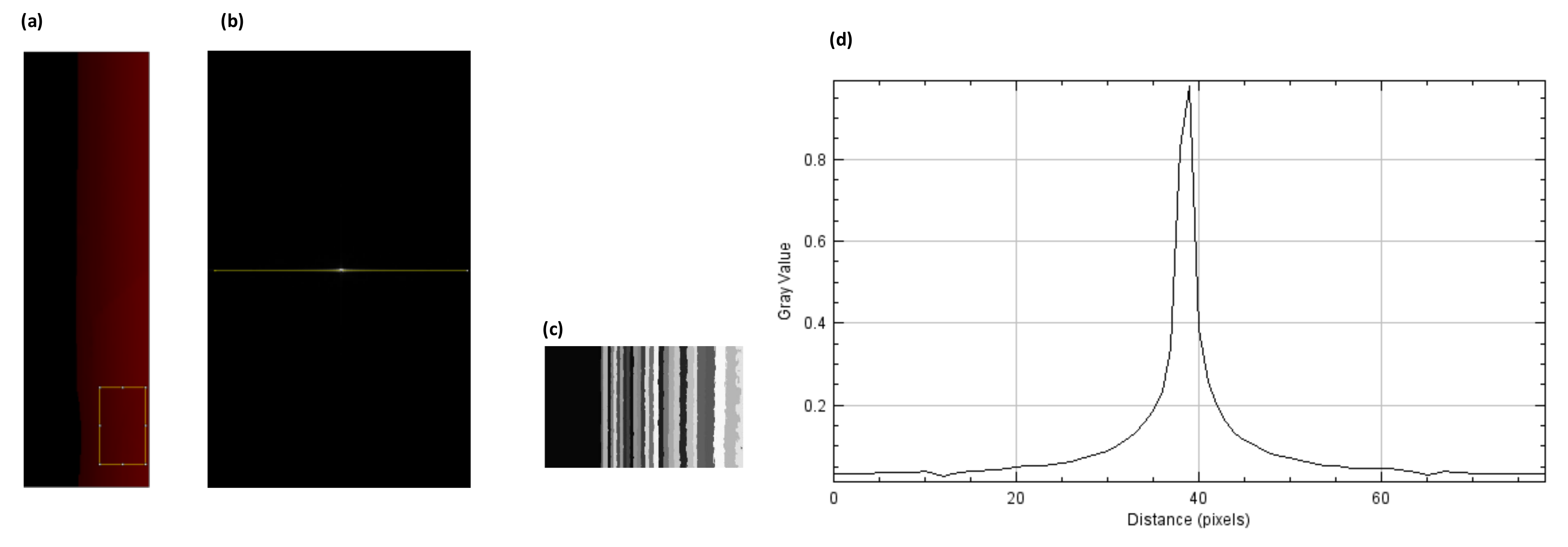
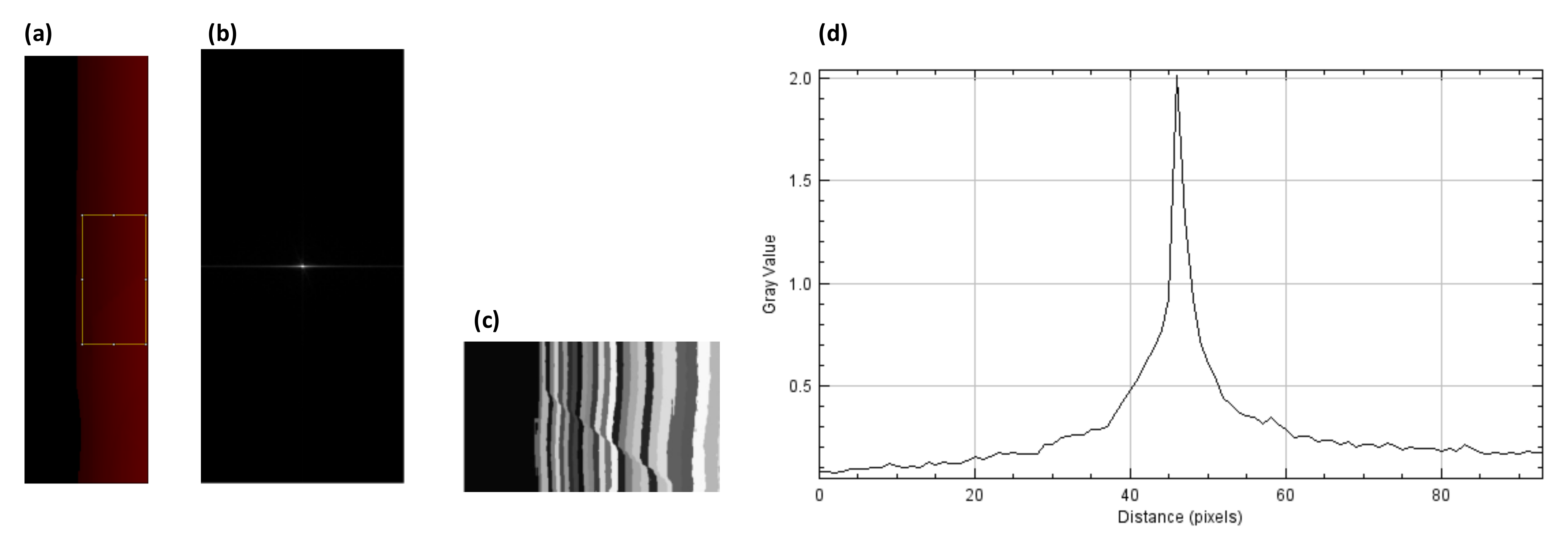
Firstly, a region of homogeneous intensity of the raw image is processed (see the yellow box in Figure 12a). The amplitude spectrum in the frequency domain is shown in Figure 12b. The image processed with K-Means, which is shown in Figure 12c, confirms that the analysed part does not show any defects, since the pixel clusters contours are perfectly parallel in the vertical direction (see Section 4.1). Figure 12d shows the DFT spectrum profile along a horizontal central slice (see yellow line in Figure 12b).
Secondly, by carrying out the same analysis on an inhomogeneous region of the raw image (shown in Figure 13a), an apparently similar DFT frequency spectrum is observed (see Figure 13b). However, as confirmed by the K-Means image shown in Figure 13c, the region is characterized by a defect.
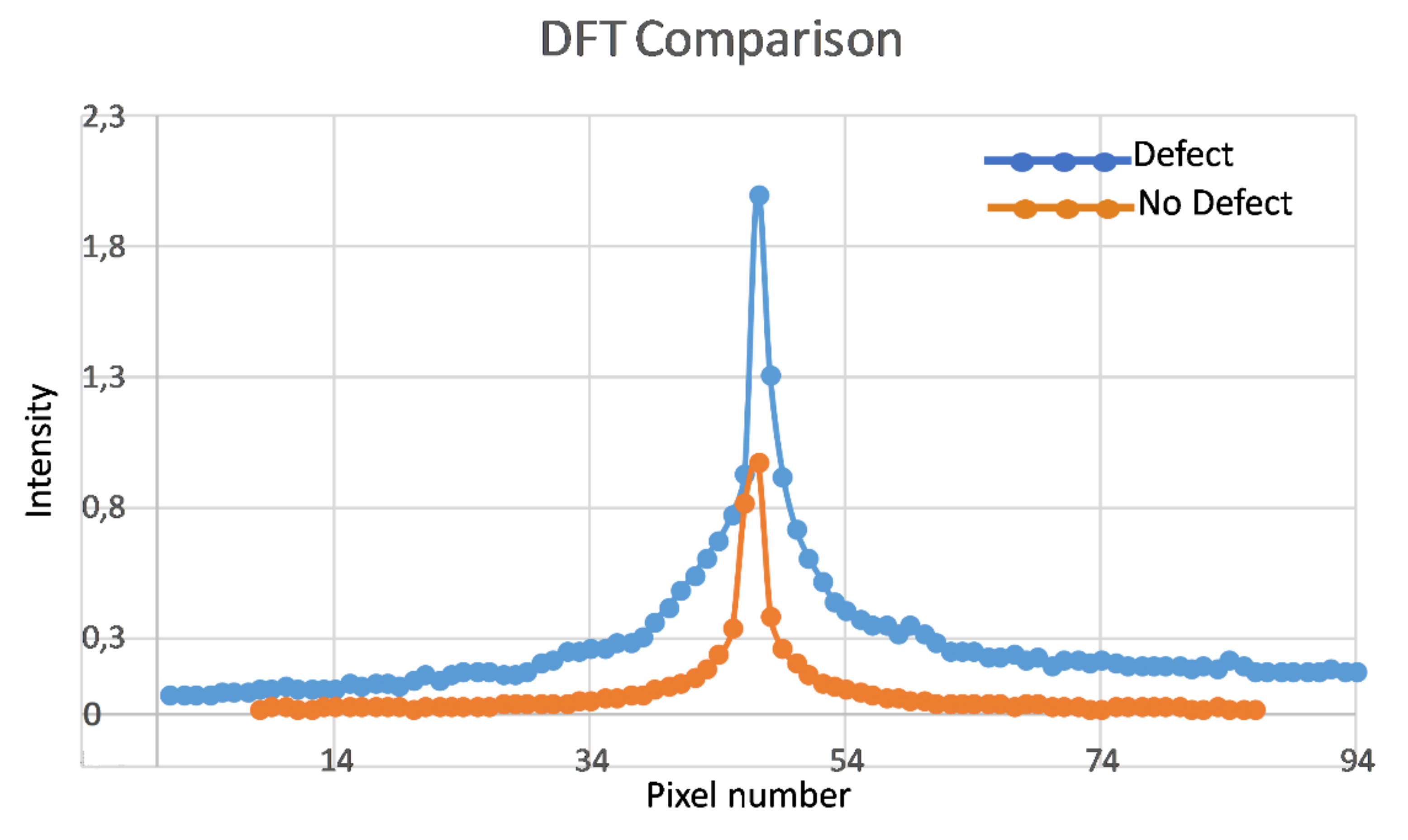
By comparing both the DFT responses in the homogeneous and inhomogeneous cases (Figure 12d or Figure 13d), Figure 14 highlights the DFT curve which is characterized by a broader profile and by a higher pixel level intensity.
While the peak intensity is related to the total intensity of the image, the difference in broadening of the amplitude spectra can be ascribed to the different range of spatial frequencies over which the images is decomposed. The images of the tire showing the defect is characterized by a broader spectrum in frequency due to the presence of large-scale changes in morphology of the spatial intensity patterns with respect to the homogenous vertical patterns. Broader amplitude spectra indicate that the spatial patterns of the image at higher spatial frequency are characterized by a higher intensity, thus implying that deviation from the homogeneous patterns are significant. The broadening of the spectrum can be measured by computing the Full Width Half Maximum (FWHM), i.e., the width in frequency of the amplitude spectrum when the amplitude reaches a value equal to half of the maximum of the spectrum. Linking the entity of the defect with the FWHM of the amplitude spectrum is beyond the scope of this paper. However, we note that the defect shown in Figure 13c is spatially extended over the whole spatial domain of the image. Therefore, the FWHM of the amplitude spectrum shown in Figure 14 is expected to be the broadest compared to the one related to spectra of images of tire sidewalls with a smaller spatial extent of defects. Due to the discrete nature of Fourier Transform of images, the amplitude spectrum can be fitted by a continuous function, such as a Gaussian function or a sinc function, in order to better characterize the broadening of the spectrum. Moreover, Figure 14 shows the profile of the DFT amplitude spectra across one slice. Generally, the amplitude spectra can be fitted in the 2d spatial frequency space by means of a bidimensional Gaussian function or the Bessel function of the first kind. It is worth remembering that the bidimensional Gaussian function and the Bessel function of the first type are the Fourier transform of a Gaussian like intensity image and a uniform image, respectively.
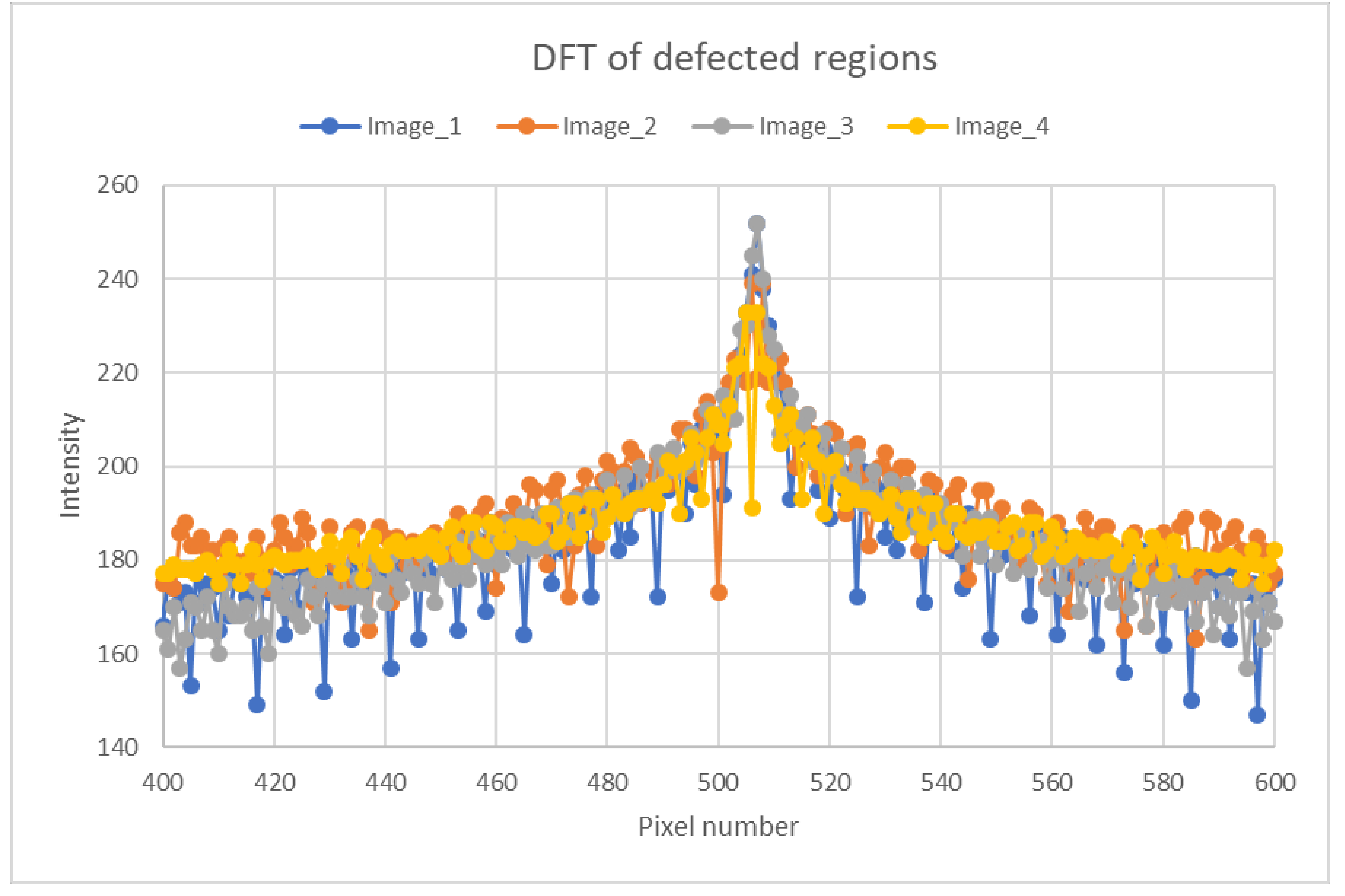
The broadening of the spectrum can be observed in all the sections of images in the dataset showing a defect. Figure 15 shows the comparison of the DFT amplitude profile across a slice for the different images of the dataset shown in Figure 7 in the image regions showing a defect (Figure 10).
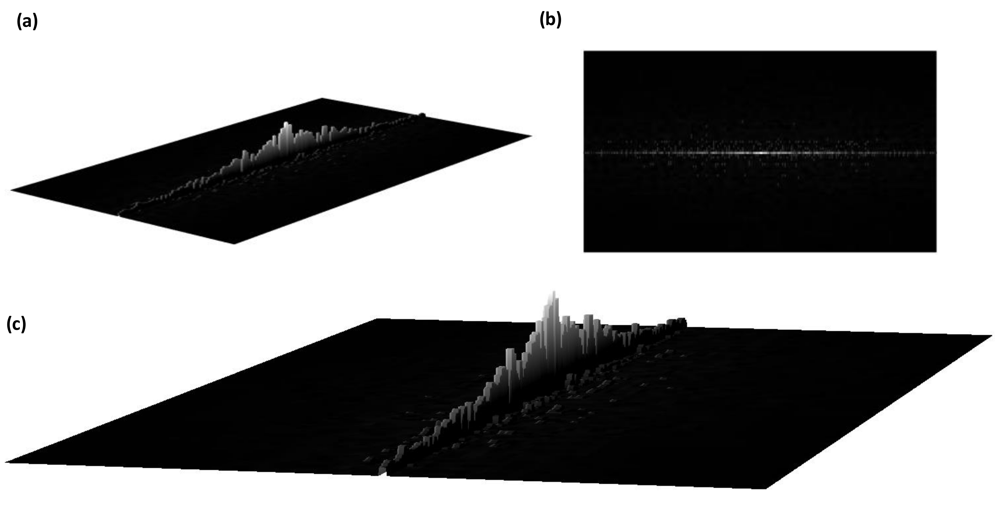
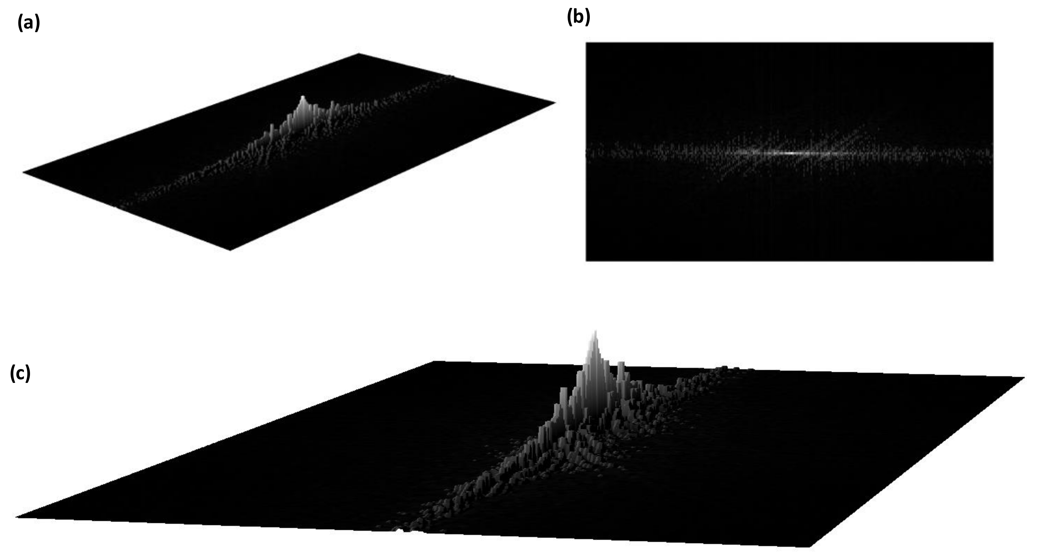
In order to further characterize the defected regions and investigate the combination of two different algorithms, the DFT approach is applied to the K-Means image shown in Figure 12c or Figure 13c. This DFT analysis contains further information about the defect characterization which can be highlighted by showing the 3D imaging of the DT in the spatial frequency. By observing Figure 16 and Figure 17, it can be noticed that the DFT spectrum of the defected region (Figure 17) is characterized by several fluctuations in amplitude. As mentioned above, the significance of the defect can be measured by fitting the DFT spectrum with a 2D function, such as a Gaussian function, and the broadening of the fitting function along the frequency axes can be related to the significance of the defect.
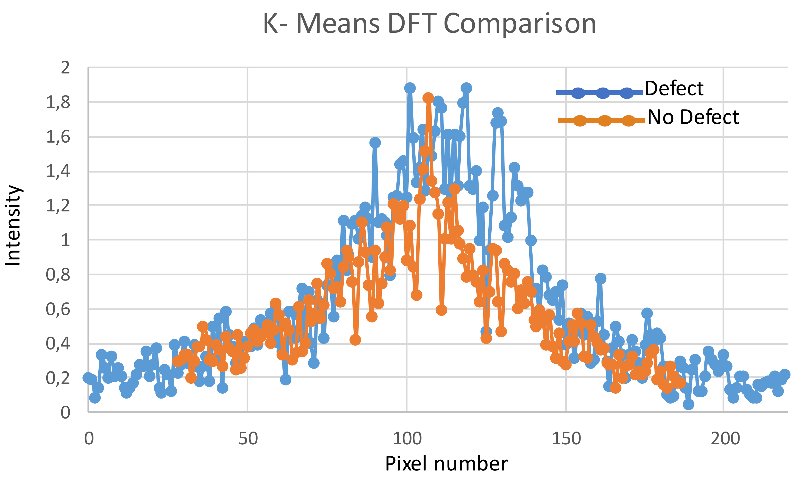
Figure 18 shows a comparison between the DFT spectra of the K-Means images of homogeneous and inhomogeneous regions (shown in Figure 16 and Figure 17), highlighting more accentuated fluctuations if compared with results of Figure 14, related to the DFT directly applied on the raw image. The DFT amplitude spectrum of the clustered image related to the image of the defected tire is characterized by a larger broadening, as observed for the DFT of the raw image.

4.3. Neural Networks

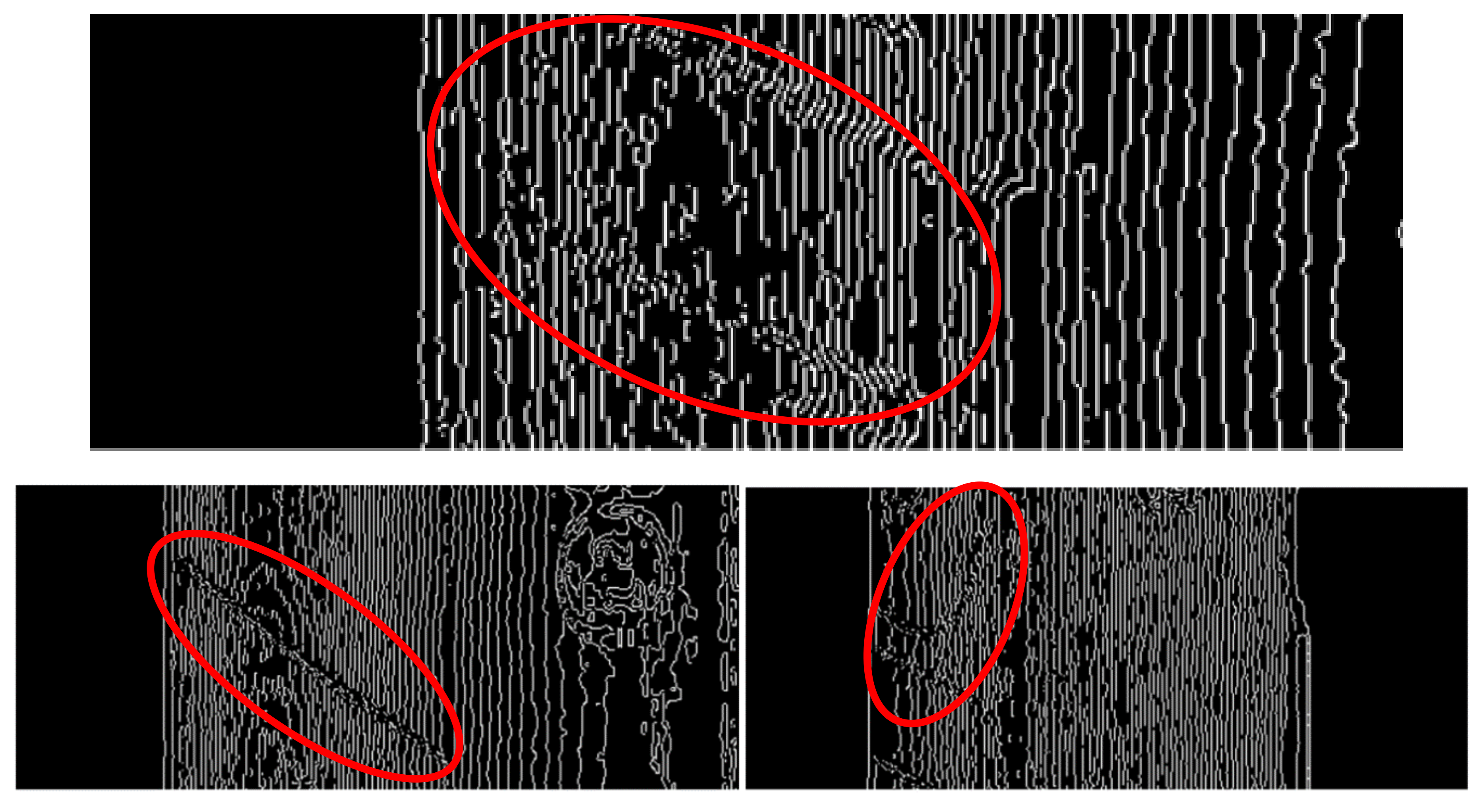
Finally, the comparative analysis is focused on the application of the neural network techniques for defect detection (Section 3.3). In Figure 19 is shown the regions of the tire sidewall in different images in the dataset where the mean squared error between the predicted and real model is maximized. The red circles indicate the region where the defect is localized on the tire sidewall with a small number of false positives.
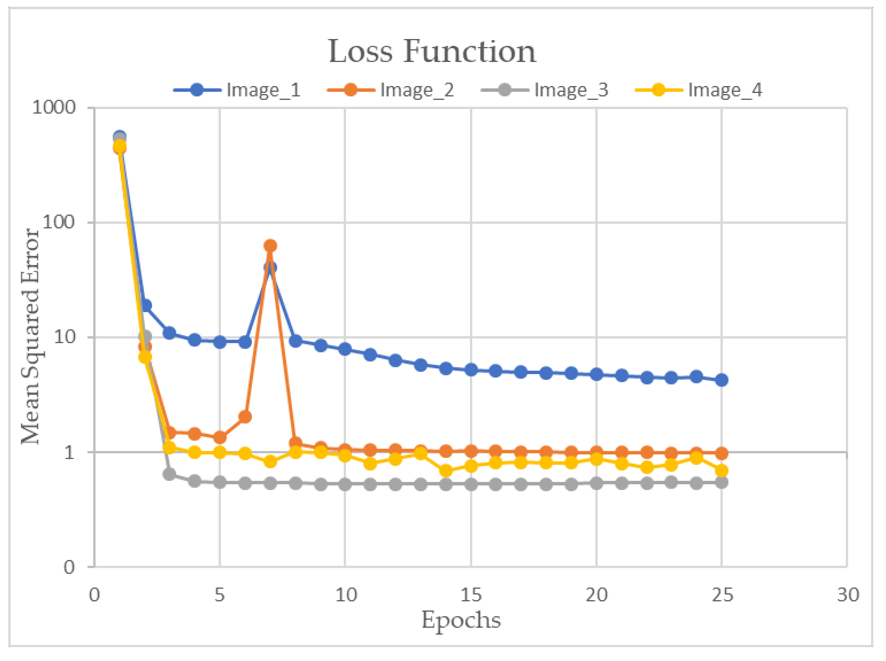
The loss function of the neural networks trained on each of the four images in the dataset are shown in Figure 20 along the epochs over which are trained. It can be noticed that the loss function decreases sharply to values close to the null values, implying that the neural networks are well trained.
Since the training of the neural network needs to be performed on each tire (due to the different texture of the tire surfaces), this method requires a larger computational effort in terms of computing time compared to other methods. On the other hand, the K-Means and DFT algorithm do not require the knowledge of the morphological feature of the whole tire, while the neural network needs to be trained over the whole tire in order to learn the main morphological features of the tire surface and identify the defects. Since the computational time could be consistent, the integration of this method in inline image vision process can be considered difficult to implement. Moreover, due to the relatively high computational time of this algorithm, a method based of a combination of neural networks and DFT or K-Means would be not convenient to implement in practice.

5. Summary and Discussion

The presented results show the DFT amplitude spectra could be used to infer the presence of a defect by analysing the broadening of the spectrum over the frequency domain. The broadening of the spectrum could be measured by computing the FWHM of the amplitude profile. Generally, the amplitude could be fitted in the bidimensional frequency domain by means of continuous functions such as Gaussian or Bessel functions, with the aim to better measure the FWHM and infer a reliable estimate of the spectrum broadening. Comparing the amplitude spectra of different region of the tire sidewall, the measure of the spectrum broadening makes the operator possible to easily find which tire regions present defects. The measure of the spectrum broadening is calibrated by identifying the expected spectrum obtained from a similar non-defective tire sidewall. This is necessary since the tire sidewalls are usually characterized by different standard spatial patterns.
Moreover, the results show that the K-Means clustering applied to the image can improve the feasibility of defect detection. The DFT of the clustered images was characterized by fluctuations with a morphology that is directly related to the significance of the defect. Moreover, our results illustrate that other methods based on neural networks could be considered as an alternative tool to detect defects on tire’s surface. However, due to the relatively large computational weight required to train the network, it was concluded that DFT and the K-Means algorithms could be used to effectively detect defects according to Industry 4.0 paradigm.
Finally, image processing techniques based on neural networks are analysed, showing a high accuracy in detecting defects but long computational time.
To summarize our findings, in Table 1 is outlined a comparison of some metrics to evaluate the performance of the three algorithms described in this paper. As previously mentioned, the K-Means and the DFT algorithm perform better than the neural network-based algorithms both in terms of computational time and because they do not require the advance knowledge of the whole image of the tire under investigation. In detail, while the accuracy of the algorithms is comparable, the computational time of the DFT or K-Means algorithm is around one-two order of magnitude lower than the computational time of the algorithm based on neural networks.
Moreover, due to the short computational time and the high accuracy, the DFT and K-Means method can be used to quickly analyse a larger number of images, making them scalable and of practical relevance for inline monitoring.

6. Conclusions

The paper is focused on the application of image processing techniques used to detect possible defects obtained after the tire-wheel rim assembling process. In detail, the following conclusions are considered from the research:
  • The comparison of the DFT, K-Means and LSTM-FC neural network algorithms reveal the possibility to in-line monitor and identify the produced defects. The mentioned techniques were successfully applied in the quality control case of the assembled tires, making possible to detect and characterize the defects generated from possible material stresses not correct tire-wheel rim coupling caused during assembling;
  • The methodology includes the individual and simultaneous application of 2D image processing techniques, i.e., the DFT approach and the K-Means image processing, which are fundamental to infer the presence of possible defects on the tire surface. All the image processing aspects, i.e., computational cost, sensitivity, error and integration, are analysed in the work;
  • The usage of LSTM-FC proves to be effective on identifying the defects of assembled tires. However, the computational cost is seen to be largely affecting the results. Further network optimisation in terms of computational time would be required to train the network, in order to make this technique more promising for an industrial application;
  • The proposed approach is suitable for image processing techniques in the field of Industry 4.0 technologies and can be applicable also to other manufacturing processes for quality check.
In conclusion, the paper suggests that the combination of DFT and K-Means provides the best method for defect detections applied on tire sidewalls in terms of accuracy and computational cost. The integration of these tools with in-line quality control based on image processing techniques is suggested to enhance the efficiency of industrial processes. Future works may be focused on the application of these methods combined with auto-actuated systems, capable to correct process values. Such application is oriented to the context of auto-adaptive Industry 5.0 facilities.

Author Contributions

Conceptualization, A.G. and A.M.; methodology, A.M. and G.D.; software, A.M. and G.D.; validation, A.M., E.C. and G. D.; formal analysis, E.C.; investigation, A.G., G.D. and A.M.; resources, A.G.; data curation, A.M. and E.C.; writing—original draft preparation, A.M.; supervision, A.G.; project administration, A.G. and A.M. All authors have read and agreed to the published version of the manuscript.

Funding

This research received no external funding.

Acknowledgments

The work has been developed in the frameworks of the Italian projects: “Innovazione di processo di assemblaggio pneumatici e potenziamento dell’ automatismo controllato con integrazione dell’ image vision per la qualità ‘AUTOMATION AND DIGITAL IMPROVEMENTS OF TIRES ASSEMBLY IN INDUSTRY 4.0’ [Innovation of tire assembly process and upgrade of the controlled automation with integration of image vision for quality check]. The authors would like to thank the Dyrecta Lab researchers C. Antonia, R. Cosmo, V. Custodero, L. D’ Alessandro, M. LeGrottaglie, A. Leogrande, A. Lombardi, V. Maritati, F. S. Massari, L. Patruno, D. D. Romagno, G. Sicolo, M. M. Sorbo, D. Suma, E. Valenzano and V. Vitti.

Conflicts of Interest

There are no conflicts of Interest.

Appendix A

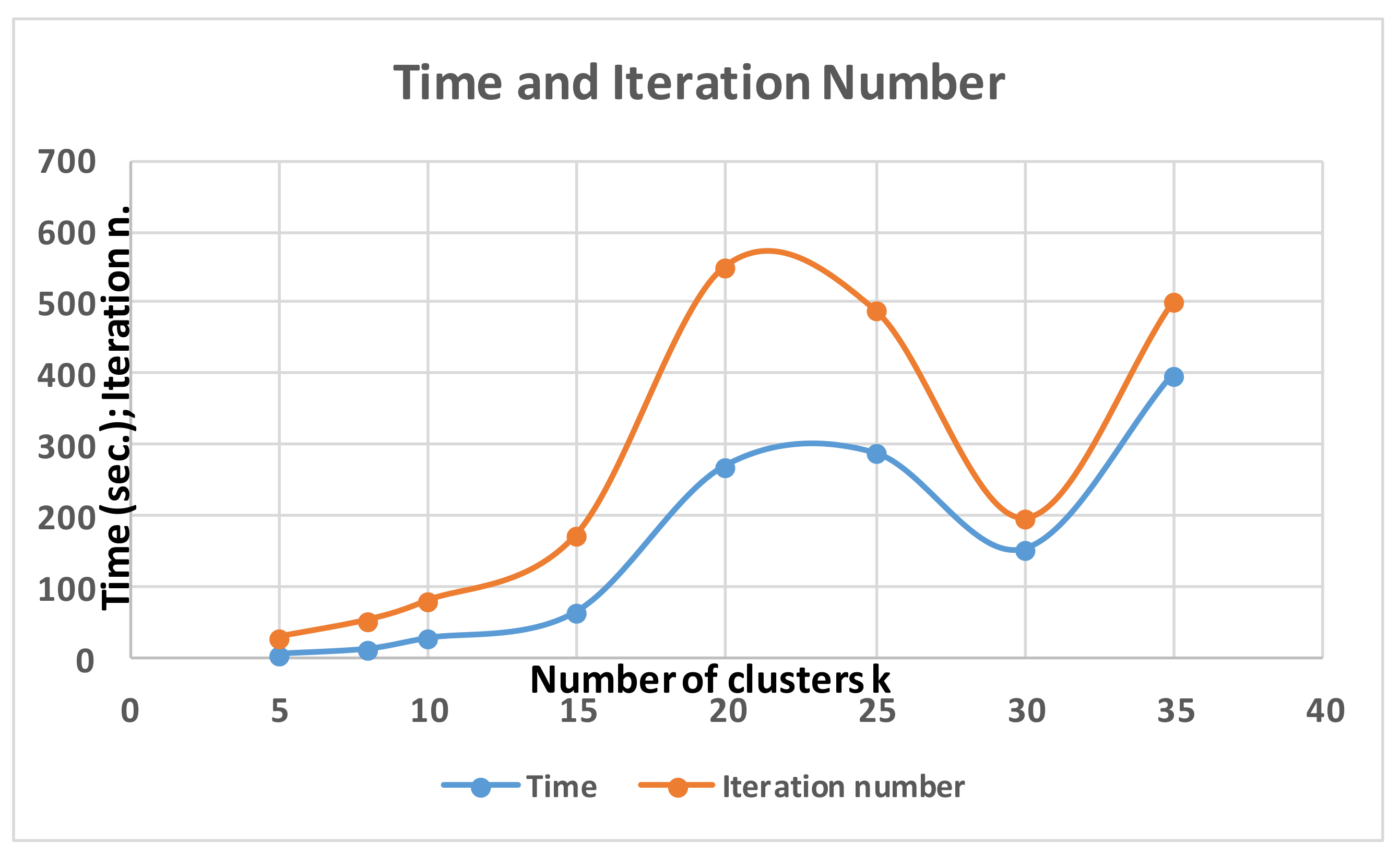
Figure A1 shows the trend of computational time and the iteration number versus the cluster number. By analysing the same image, the computational cost is observed to increase up to K = 20. Then, it decreases and increases again for K larger than 30. The value K = 30 was assumed to be enough for image analysis, but K = 35 provided a better processing resolution.
Figure A1. Time and iteration number versus the cluster number k (image processing of the same image).
Information 11 00257 g0a1
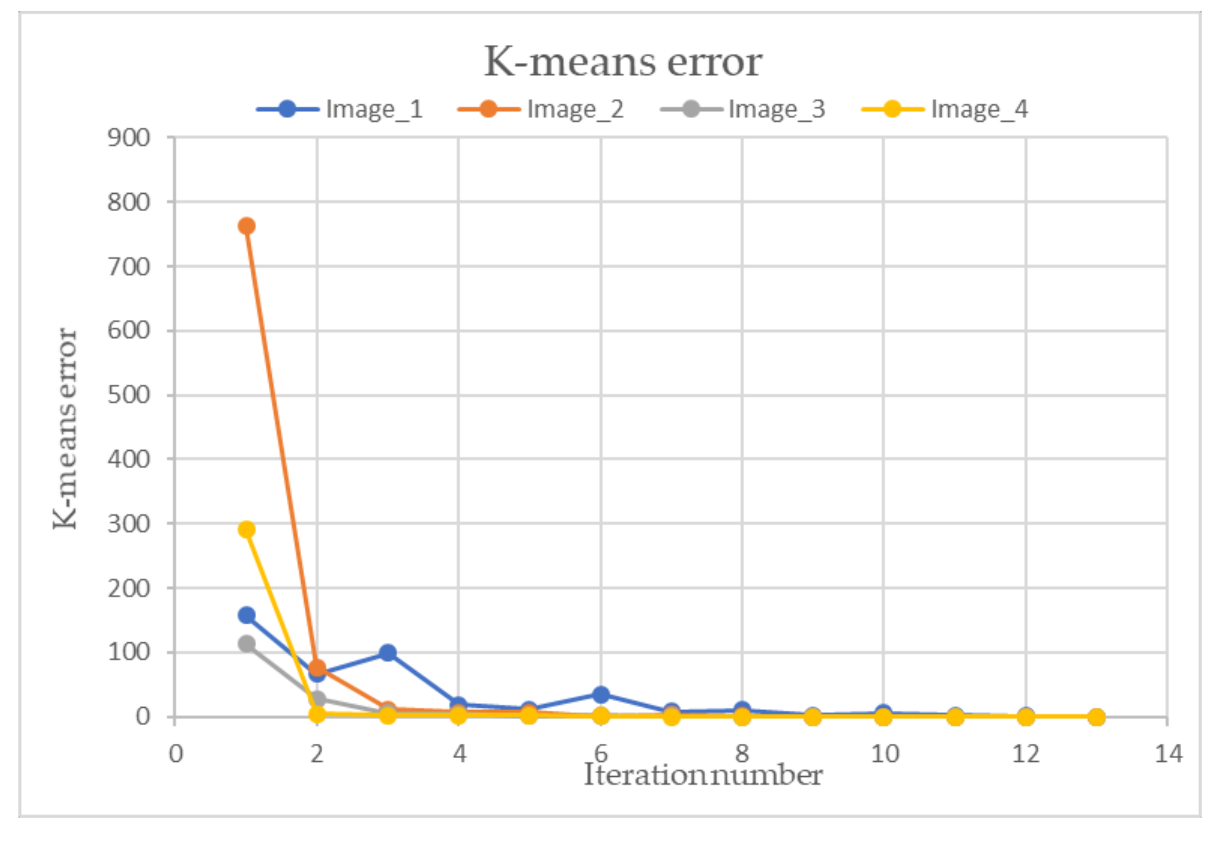
In Figure A2 is illustrated an example of cluster error trend versus the iteration number. It can be noticed that, in all the cases, the error approaches the null value after few iteration steps.
Figure A2. Cluster error versus the iteration number (for K=5) for the different images in the dataset.
Information 11 00257 g0a2

References

  1. Chavda, A.; Patil, P.M.Y. Increased Productivity of Tyre Manufacturing Process using Lean Methodology. In Proceedings of the International Conference on Current Trends in Technology, NUiCONE–2011, Ahmedabad, Gujarat, India, 8–10 December 2011; pp. 382–481. [Google Scholar]
  2. Womack, J.P.; Jones, D.T. Lean Thinking; Mass: Brookline, MA, USA, 2003; ISBN 0774779497. [Google Scholar]
  3. Womack, J.P.; Jones, D.T. Lean Journal of the Operational Research Society. Thinking—Banish Waste and Create Wealth in your Corporation. J. Oper. Res. Soc. 1997, 48, 1148. [Google Scholar] [CrossRef]
  4. Tire Building Machine, White Paper Rockwell Automation Tire Building Machine Reduce Design Time and Improve TCO for Tire Manufacturers 2013. Available online: https://docplayer.net/21471375-Tire-building-machine.html (accessed on 8 May 2020).
  5. U.S. Department of Transportation the Pneumatic Tire. Available online: https://www.nhtsa.gov/staticfiles/safercar/pdf/PneumaticTire_HS-810-561.pdf (accessed on 8 May 2020).
  6. Cao, M.; Wang, G.; Sun, L. Research on Key Technology of New Concept Tyre Building Production Line. Int. J. Intell. Syst. Appl. 2012, 4, 46–52. [Google Scholar]
  7. Beckhoff PC Based Control for Tire And Rubber Industry. Available online: https://m.beckhoff.com/english/applicat/rubber_text.htm (accessed on 5 September 2019).
  8. Swedberg, C. The HF RFID solution can be used to monitor tire production, as well as to manage the trays used to transport and store uncured tires. Available online: https://www.rfidjournal.com/articles/pdf?14554 (accessed on 5 September 2019).
  9. Bahmankhah, B.; Alvelos, H. Exploring the Potential of Quality Tools in Tire Retreading Industry: A Case Study. Int. J. Eng. Sci. Technol. 2011, 3, 5337–5345. [Google Scholar]
  10. Chen, P.; Shubinsky, G.D.; Jan, K.-H.; Chen, C.-A.; Sidla, O.; Poelzleitner, W. Inspection of tire tread defects using image processing and pattern recognition techniques. In Proceedings of the SPIE 2063, Vision, Sensors, and Control for Automated Manufacturing Systems, Boston, Massachusetts, 9–10 September 1993; Breidenthal, S.S., Desrochers, A.A., Eds.; pp. 14–21. [Google Scholar]
  11. Donahue, E.; Quach, T.-T.; Potter, K.; Martinez, C.; Smith, M.D.; Turner, C. Deep learning for automated defect detection in high-reliability electronic parts. In Proceedings of the Applications of Machine Learning, San Diego, CA, USA, 11–15 August 2019; Zelinski, M.E., Taha, T.M., Howe, J., Awwal, A.A., Iftekharuddin, K.M., Eds.; p. 4. [Google Scholar] [CrossRef]
  12. Schlegl, T.; Seeböck, P.; Waldstein, S.M.; Langs, G.; Schmidt-Erfurth, U. f-AnoGAN: Fast unsupervised anomaly detection with generative adversarial networks. Med. Image Anal. 2019, 54, 30–44. [Google Scholar] [CrossRef] [PubMed]
  13. Xu, H.; Chen, W.; Zhao, N.; Li, Z.; Bu, J.; Li, Z.; Liu, Y.; Zhao, Y.; Pei, D.; Feng, Y.; et al. Unsupervised Anomaly Detection via Variational Auto-Encoder for Seasonal KPIs in Web Applications. In Proceedings of the 2018 World Wide Web Conference, Lyon, France, 23–27 April 2018. [Google Scholar]
  14. Nguyen, Q.P.; Lim, K.W.; Divakaran, D.M.; Kian Hsiang Low, M.C.C. GEE: A Gradient-based Explainable Variational Autoencoder for Network Anomaly Detection. In Proceedings of the 2019 IEEE Conference on Communications and Network Security (CNS), Washington, DC, USA, 10–12 June 2019. [Google Scholar]
  15. An, J.; Cho, S. Variational Autoencoder based Anomaly Detection using Reconstruction Probability. 2015. Available online: http://dm.snu.ac.kr/static/docs/TR/SNUDM-TR-2015-03.pdf (accessed on 8 May 2020).
  16. Zimmerer, D.; Petersen, J.; Kohl, S.A.A.; Maier-Hein, K.H. A Case for the Score: Identifying Image Anomalies using Variational Autoencoder Gradients. In Proceedings of the 32nd Conference on Neural Information Processing Systems (NeurIPS 2018), Montreal, QC, Canda, 3–8 December 2018. [Google Scholar]
  17. Bergmann, P.; Löwe, S.; Fauser, M.; Sattlegger, D.; Steger, C. Improving Unsupervised Defect Segmentation by Applying Structural Similarity to Autoencoders. In Proceedings of the 14th International Joint Conference on Computer Vision, Imaging and Computer Graphics Theory and Applications, SCITEPRESS—Science and Technology Publications, Prague, Czech Republic, 25–27 Febuary 2019; pp. 372–380. [Google Scholar]
  18. Dehaene, D.; Frigo, O.; Combrexelle, S.; Eline, P. Iterative energy-based projection on a normal data manifold for anomaly localization. In Proceedings of the The International Conference on Learning Representations (ICLR 2020), Addis Ababa, Ethiopia, 26–30 April 2020. [Google Scholar]
  19. Gros, X.E. Technical Note: Detection of delamination in tyres using eddy currents. Proc. Inst. Mech. Eng. Part D J. Automob. Eng. 1997, 211, 79–82. [Google Scholar] [CrossRef]
  20. Gray, W.H.; Dumont, C.; Abidi, M.A. Simulation of a tire inspection system. Available online: https://www.semanticscholar.org/paper/SIMULATION-OF-A-TIRE-INSPECTION-SYSTEM-Gray-Dumont/33a8d7badf8984d4bb265f12346b1c9f379f39b2 (accessed on 8 May 2020).
  21. Cicala, G.; Massaro, A.; Velardi, L.; Senesi, G.S.; Valentini, A. Self-Assembled Pillar-like Structures in Nanodiamond Layers by Pulsed Spray Technique. ACS Appl. Mater. Interfaces 2014, 6, 21101–21109. [Google Scholar] [CrossRef]
  22. Beniguel, J.F.; Gaudin, A.; Abbadi, Z.; Le Pen, D. Tire-Wheel-Cavity dynamic model for Structure-borne road noise simulation. In Proceedings of the Acoustics 2012 Nantes Conference, Nantes, France, 23–27 April 2012. [Google Scholar]
  23. Massaro, A.; Vitti, V.; Galiano, A. Automatic Image Processing Engine Oriented on Quality Control of Electronic Boards. Signal Image Process. Int. J. 2018, 9, 1–14. [Google Scholar] [CrossRef]
  24. Ashok, V.; Vinod, D.S.. Using K-Means Cluster and Fuzzy C Means for Defect. Int. J. Comput. Eng. Technol. 2014, 11–19. [Google Scholar]
  25. Bulnes, F.G.; Usamentiaga, R.; Garcia, D.F.; Molleda, J. An efficient method for defect detection during the manufacturing of web materials. J. Intell. Manuf. 2016, 27, 431–445. [Google Scholar] [CrossRef]
  26. Xu, D.; Tian, Y. A Comprehensive Survey of Clustering Algorithms. Ann. Data Sci. 2015, 2, 165–193. [Google Scholar] [CrossRef] [Green Version]
  27. Pal, N.R.; Pal, S.K. A review on image segmentation techniques. Pattern Recognit. 1993, 26, 1277–1294. [Google Scholar] [CrossRef]
  28. Fan, J.; Yau, D.K.Y.; Elmagarmid, A.K.; Aref, W.G. Automatic image segmentation by integrating color-edge extraction and seeded region growing. IEEE Trans. Image Process. 2001, 10, 1454–1466. [Google Scholar] [CrossRef] [PubMed] [Green Version]
  29. Massaro, A.; Galiano, A.; Meuli, G.; Massari, S.F. Overview and Application of Enabling Technologies Oriented on Energy Routing Monitoring, on Network Installation and on Predictive Maintenance. Int. J. Artif. Intell. Appl. 2018, 9, 1–20. [Google Scholar] [CrossRef]
  30. Arora, S.; Kaur, P.; Arora, P. Economical Maintenance and Replacement Decision Making in Fleet Management using Data Mining. SIJ Trans. Comput. Sci. Eng. Appl. 2013, 1, 09–20. [Google Scholar] [CrossRef]
  31. IJ Plugins K-means Clustering. Available online: http://ij-plugins.sourceforge.net/plugins/segmentation/k-means.html (accessed on 10 September 2019).
  32. Morrison, N. Introduction to Fourier Analysis; Wiley: London, UK, 1994. [Google Scholar]
  33. Marion, A. Introduction to Image Processing; Springer US: Boston, MA, USA, 1991; ISBN 978-0-442-31202-2. [Google Scholar]
  34. Oberst, U. The Fast Fourier Transform. SIAM J. Control Optim. 2007, 46, 496–540. [Google Scholar] [CrossRef]
  35. Shapiro, L.G. Computer vision: The last 50 years. Int. J. Parallel Emergent Distrib. Syst. 2018, 1–6. [Google Scholar] [CrossRef]
  36. Fanti, G.; Basso, R. A diagnostic tool for the quality control of gear pumps. Int. J. Mater. Prod. Technol. 2004, 20, 193. [Google Scholar] [CrossRef]
  37. LeCun, Y.; Bengio, Y.; Hinton, G. Deep learning. Nature 2015, 521, 436–444. [Google Scholar] [CrossRef]
  38. Wang, R.; Guo, Q.; Lu, S.; Zhang, C. Tire Defect Detection Using Fully Convolutional Network. IEEE Access 2019, 7, 43502–43510. [Google Scholar] [CrossRef]
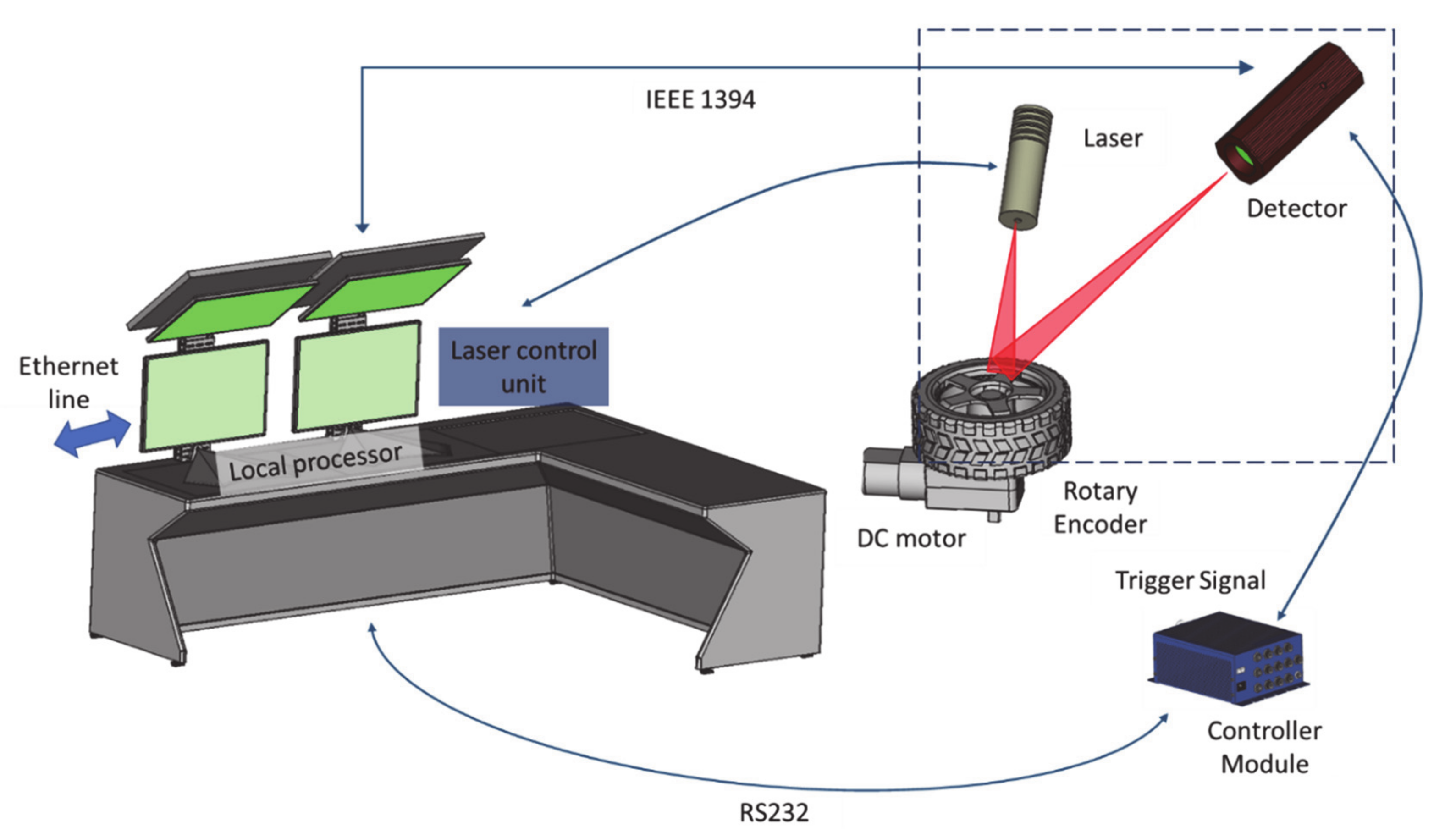
Figure 1. Scheme showing the in-line inspection system. Optical tools are used for quality control of the assembled tires.
Information 11 00257 g001
Figure 2. Pictures showing (a) the apparatus used for quality control of the tire-wheel assembly and (b) the measuring phase seen from the top of the control apparatus.
Information 11 00257 g002
Figure 3. Pictures showing the (a) 3D reconstruction operated by the in-line quality control apparatus and (b) conversion to a 2D picture.
Information 11 00257 g003
Figure 4. Flowchart describing the methodological approach followed from the present research.
Information 11 00257 g004
Figure 5. Overview of the architecture of the stack of neural networks.
Information 11 00257 g005
Figure 6. (a) Tire positioned on the rotary encoder and areas detected by the camera; (b) part of the raw linearized image of the tire sidewall containing assembly defect.
Information 11 00257 g006
Figure 7. Dataset of images of tire sidewalls.
Information 11 00257 g007
Figure 8. K-Means image processing of a homogenous region with different K cluster number.
Information 11 00257 g008
Figure 9. K-Means image processing: (a) distributed stress defect; (b) local defects; (c) partially distributed local defect.
Information 11 00257 g009
Figure 10. K-Means image processing of the images in the dataset with K=30.
Information 11 00257 g010
Figure 11. K-Means image processing of noisy images with (top) Gaussian blurring and (bottom) white noise with a dispersion factor of 8 pixels.
Information 11 00257 g011
Figure 12. (a) Tire sidewall linearized image selecting a homogeneous region. (b) Discrete Fourier Transform (DFT) transform. (c) K-Means image processing of the selected homogeneous region (K = 35). (d) DFT power frequency spectrum across the yellow line shown in Figure 12b.
Information 11 00257 g012
Figure 13. (a) Tire sidewall linearized image selecting an inhomogeneous region. (b) Frequency spectrum of the DFT transform. (c) K-Means image processing of the selected homogeneous region (K=35). (d) DFT frequency spectrum.
Information 11 00257 g013
Figure 14. Comparison between the DFT amplitude spectra shown in Figure 12d or Figure 13d.
Information 11 00257 g014
Figure 15. Comparison of DFT amplitude profile of the images shown in Figure 6.
Information 11 00257 g015
Figure 16. (ac) DFT of the K-Means image: different perspectives of the 3D DFT processing of the homogeneous region.
Information 11 00257 g016
Figure 17. (ac) DFT of the K-Means image: different perspectives of the 3D DFT processing of the inhomogeneous region highlighting amplitude fluctuations.
Information 11 00257 g017
Figure 18. Comparison between the K-Means DFT amplitude spectrum of the K-Means image (K= 35) for defect and no defect region, respectively.
Information 11 00257 g018
Figure 19. Defect detections in different images. Red areas indicate the position of defects. (Above) Common defect; (below left) extended defect; (below right) other defect type with different orientation.
Information 11 00257 g019
Figure 20. Semi-log plot of the loss function for the neural networks trained over the four different images in the dataset.
Information 11 00257 g020
Table 1. Comparison of performance indicators of the three different algorithms presented in the paper.
AlgorithmAccuracyComputational timeAdvance Knowledge of the Whole Image
DFTHigh< 1 snot required
K-MeansHighAround 10 snot required
LSTM-FCHigh> 1 minrequired