Dynamic Estimation of Saturation Flow Rate at Information-Rich Signalized Intersections


Abstract
:1. Introduction
2. Related Works
2.1. U.S. Highway Capacity Manual Methods
2.2. Improved Adjustment Methods
2.3. Estimated Departure Headway Methods
2.4. Statistical and Physical Methods
3. Methods
3.1. Conventional Method
3.2. Neural Network Method
3.2.1. Training of the Neural Network
3.2.2. Performance Evaluation
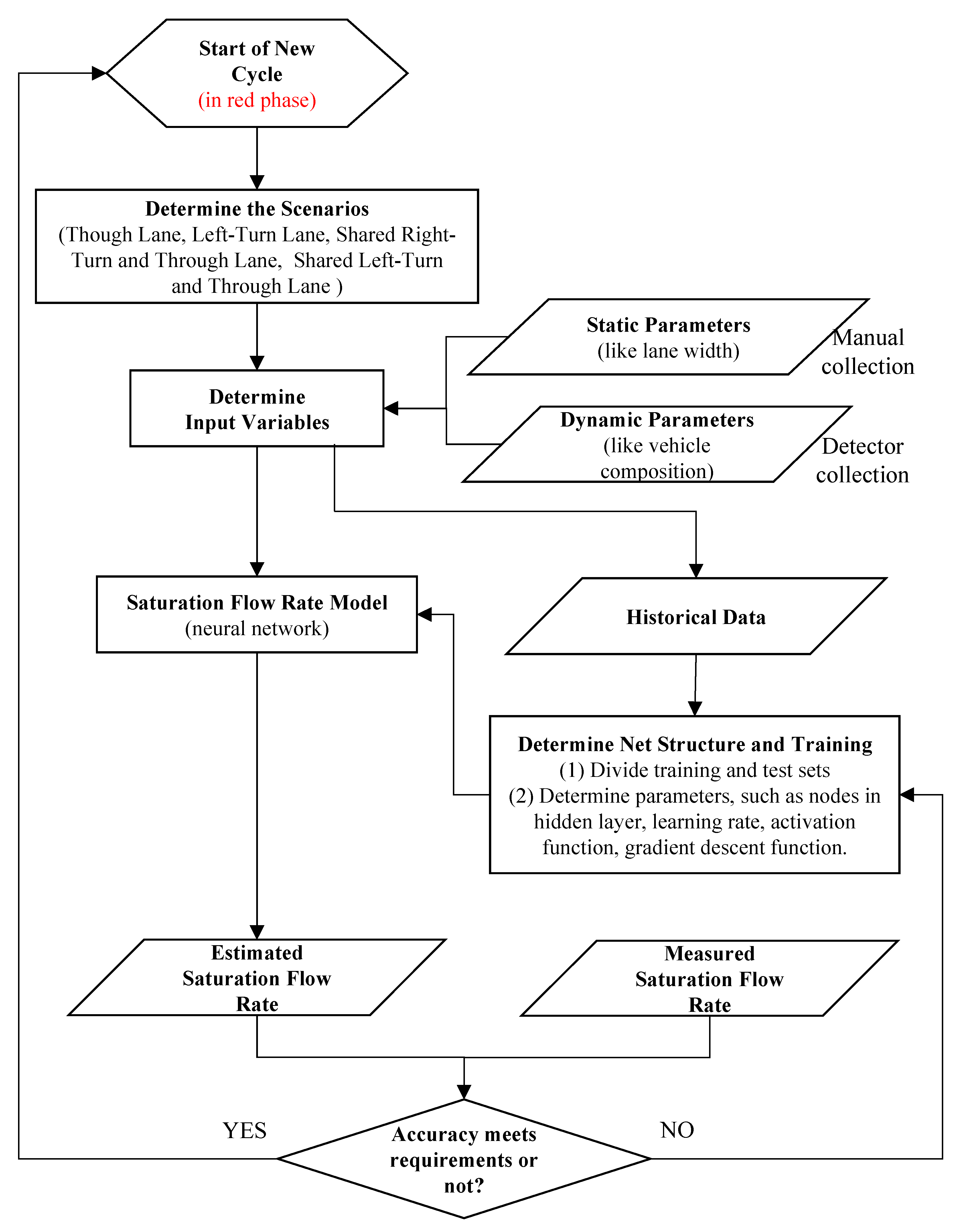
3.3. Proposed Model
3.3.1. Selection of Input Variables
3.3.2. Model Structure
4. Data Collection
5. Results and Discussion
5.1. Data Summary
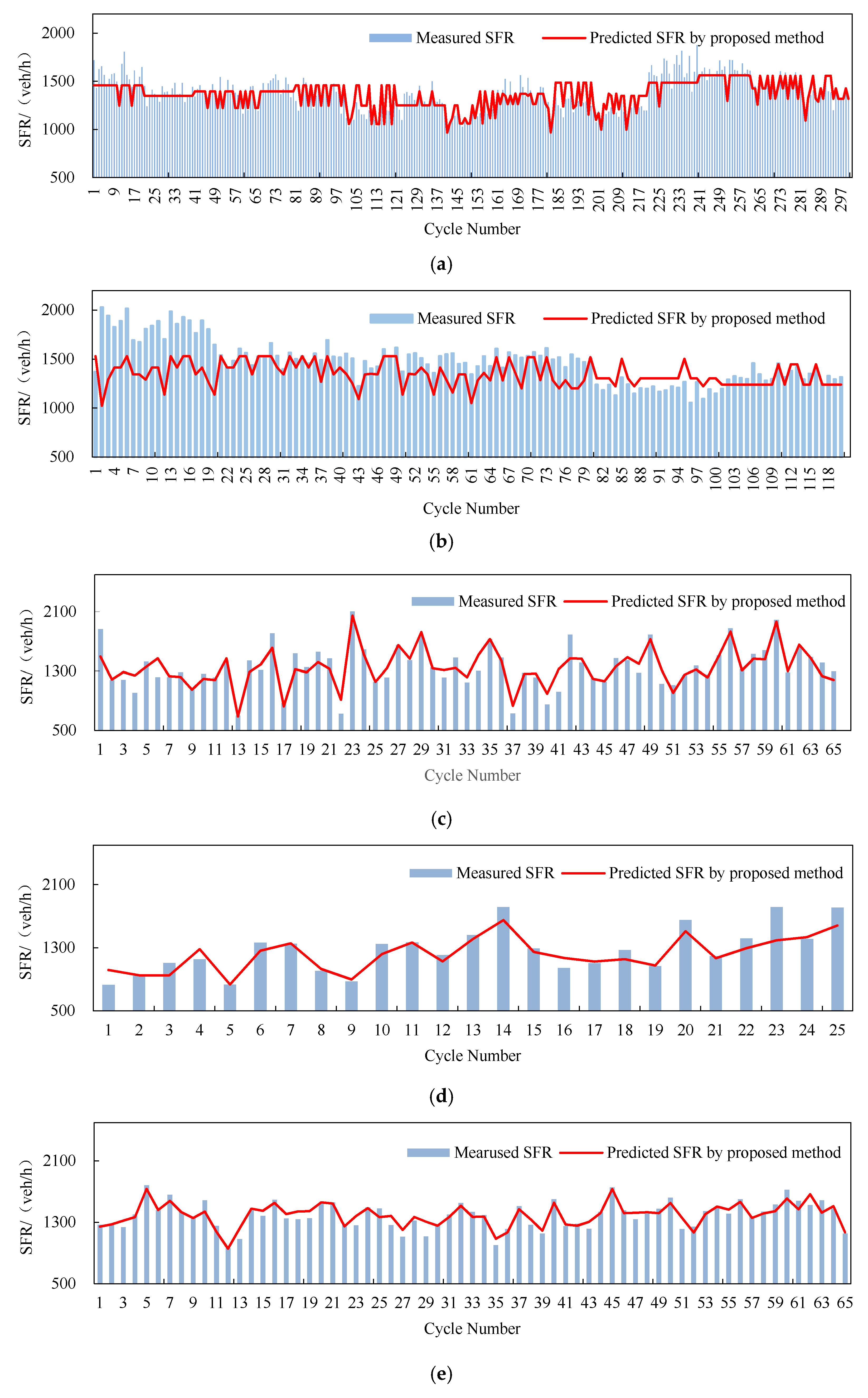
5.2. Saturation Flow Rate Estimation Model with a Neurnal Network
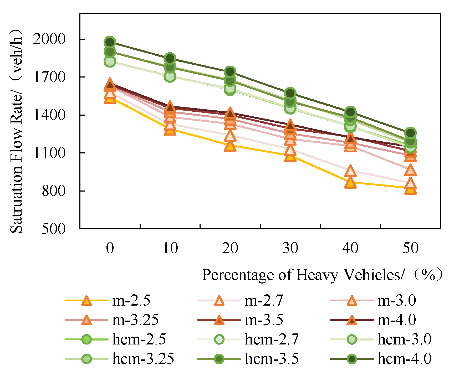
5.3. Comparison of Proposed Method and Conventional Method
5.4. Potential Applications
6. Conclusions
Author Contributions
Funding
Conflicts of Interest
Appendix A
References
- Beijing Transport Institute. 2019 Beijing Transport Annual Report; Beijing Transport Institute: Beijing, China, 2019; pp. 1–2. [Google Scholar]
- Xia, X.; Ma, X.; Wang, J. Control Method for Signalized Intersection with Integrated Waiting Area. Appl. Sci. 2019, 9, 968. [Google Scholar] [CrossRef] [Green Version]
- Transportation Research Board. Highway Capacity Manual; National Research Council: Washington, DC, USA, 2010; p. 34. ISBN 978-0-309-16077-3. Available online: www.trb.org (accessed on 25 March 2020).
- Qin, Z.; Zhao, J.; Liang, S.; Yao, J. Impact of Guideline Markings on Saturation Flow Rate at Signalized Intersections. J. Adv. Transp. 2019, 2019, 1–14. [Google Scholar] [CrossRef]
- Anusha, C.; Verma, A.; Kavitha, G. Effects of two-wheelers on saturation flow at signalized intersections in developing countries. J. Transp. Eng. 2012, 139, 448–457. [Google Scholar] [CrossRef]
- Shao, C.; Rong, J.; Liu, X. Study on the Saturation Flow Rate and Its Influence Factors at Signalized Intersections in China. In Proceedings of the 6th International Symposium on Highway Capacity and Quality of Service, Stockholm, Sweden, 28 June–3 July 2011. [Google Scholar]
- Wang, Y.; Rong, J.; Zhou, C.; Chang, X.; Liu, S. An Analysis of the Interactions between Adjustment Factors of Saturation Flow Rates at Signalized Intersections. Sustainability 2020, 12, 665. [Google Scholar] [CrossRef] [Green Version]
- Lewis, E.; Rahim, F. Saturation Flow Rate Study at Signalized Intersections in Panama. In Proceedings of the 86th Annual Meeting of the Transportation Research Board, Washington, DC, USA, 21–25 January 2007; Available online: https://trid.trb.org/view/802745 (accessed on 25 March 2020).
- Yang, D.; Luo, J.; Liu, C.; Duan, Z. Dynamic Extraction Method of Saturation Flow Rate at Signalized Intersection. J. Traffic Transp. Eng. 2013, 13, 98–103. [Google Scholar]
- Wang, L.; Wang, Y.; Bie, Y. Automatic Estimation Method for Intersection Saturation Flow Rate Based on Video Detector Data. J. Adv. Transp. 2018, 2018, 1–10. [Google Scholar] [CrossRef]
- Radhakrishnan, P.; Mathew, T. Passenger Car Units and Saturation Flow Models for Highly Heterogeneous Traffic at Urban Signalized Intersections. Transportmetrica 2011, 7, 141–162. [Google Scholar] [CrossRef]
- Tong, H.; Hung, W. Neural Network Modeling of Vehicle Discharge Headway at Signalized Intersection: Model Descriptions and Results. Transp. Res. Part A Policy Pract. 2002, 36, 17–40. [Google Scholar] [CrossRef]
- Saha, A.; Chakraborty, S.; Chandra, S.; Ghosh, I. Kriging Based Saturation Flow Models for Traffic Conditions in Indian Cities. Transp. Res. Part A Policy Pract. 2018, 118, 38–51. [Google Scholar] [CrossRef]
- Shao, C.; Liu, X. Estimation of Saturation Flow Rates at Signalized Intersections. Discret. Dyn. Nat. Soc. 2012, 2012, 1–10. [Google Scholar] [CrossRef]
- Murat, Y.; Cetin, M. A New Perspective for Saturation Flows at Signalized Intersections. Period. Polytech. Civ. Eng. 2019, 63, 296–307. [Google Scholar] [CrossRef]
- Hossain, M. Estimation of Saturation Flow at Signalised Intersections of developing cities: A micro-simulation modelling approach. Transp. Res. Part A Policy Pract. 2001, 35, 123–141. [Google Scholar] [CrossRef]
- Gao, K.; Han, F.; Dong, P.; Xiong, N.; Du, R. Connected vehicle as a mobile sensor for real time queue length at signalized intersections. Sensors 2019, 9, 2059. [Google Scholar] [CrossRef] [PubMed] [Green Version]
- Guo, Q.; Li, L.; Ban, X.J. Urban traffic signal control with connected and automated vehicles: A survey. Transp. Res. Part C Emerg. Technol. 2019, 101, 313–334. [Google Scholar] [CrossRef]
- Zheng, J.; Liu, H.X. Estimating Traffic Volumes for Signalized Intersections Using Connected Vehicle Data. Transp. Res. Part C Emerg. Technol. 2017, 79, 347–362. [Google Scholar] [CrossRef] [Green Version]
- Ren, C.; Wang, J.; Qin, L.; Li, S.; Cheng, Y. A Novel Left-Turn Signal Control Method for Improving Intersection Capacity in a Connected Vehicle Environment. Electronics 2019, 8, 1058. [Google Scholar] [CrossRef] [Green Version]
- Ministry of Transport of the People’s Republic of China Issues Notice to Promote ETC Installation. Available online: http://www.gov.cn/xinwen/2019-05/24/content_5394287.htm (accessed on 24 May 2019).
- Yang, H.; Zhang, L.; Cheng, L.; Gao, C. Research on Travel Features of Car Based on RFID Big Data in Chongqing Main City. In Proceedings of the International Conference on Green Intelligent Transportation System and Safety, Changchun, China, 1–2 July 2017. [Google Scholar]
- Accenture: Mobility As a Service. Available online: https://www.accenture.com/cn-en/insight-mobility-automotive-ecosystem (accessed on 25 March 2020).
- Chen, P.; Qi, H.; Sun, J. Investigation of Saturation Flow on Shared Right-Turn Lane at Signalized Intersections. Transp. Res. Rec. 2014, 2461, 66–75. [Google Scholar] [CrossRef]
- Tongji University. Code for Planning of Intersections on Urban Roads (GB50647-2011); China Planning Press: Beijing, China, 2011; p. 77. Available online: http://www.ccsn.org.cn (accessed on 25 March 2020).
- Karlaftis, M.; Vlahogianni, E. Statistical Methods versus Neural Networks in Transportation Research: Differences, Similarities and Some Insights. Transp. Res. Part C Emerg. Technol. 2011, 19, 387–399. [Google Scholar] [CrossRef]
- Pu, Q.; Huang, Q.; Yang, P. Statistical Model for Delay of Intersection. J. Tongji Univ. 2005, 33, 1309. [Google Scholar]
- Tarko, A.; Rouphail, N.; Akcelik, R. Overflow delay at a signalized intersection approach influenced by an upstream signal: An analytical investigation. Transp. Res. Rec. 1993, 1993, 82–89. [Google Scholar]
- Hurdle, V. Signalized intersection delay models—A primer for the uninitiated. Transp. Res. Rec. 1984, 971, 96–105. [Google Scholar]
- He, J.; Hou, Z. Ant colony algorithm for traffic signal timing optimization. Adv. Eng. Softw. 2012, 43, 14–18. [Google Scholar] [CrossRef]


| Variables | Definition | Ranges |
|---|---|---|
| X1 | Lane width (m) | No specific range |
| X2 | Percentage of heavy vehicles | 0–0.5 |
| X3 | Interference in multiple through lanes | 0, 1 |
| X4 | Percentage of turning vehicles in the lane group | 0–1.0 |
| X5 | Disturbed pedestrians | No specific range |
| X6 | Disturbed bicycles | No specific range |
| X7 | Opposing vehicles | No specific range |
| Scenario 1: TH 1 | Scenario 2: TH-RT 2 | Scenario 3: TH-LT 3 | |
|---|---|---|---|
| Intersection Name | Shiliuzhuang Rd 4 and Liuxiang Rd | Chegongzhuangxi Rd and Shoudutiyuguannan Rd | Andingmenwai St 5 and Waiguanxie St |
| Westbound Lanes in Approaches | 1U 6+2LT 7+2TH+1RT 8 | 1LT+2TH+1TH-RT+1RT | 1LT-TH-RT |
| Eastbound Lanes in Approaches | 1LT+1TH+1RT | 1LT+2TH+1RT | 1LT-TH+1RT |
| Northbound Lanes in Approaches | 2LT+4TH+1RT | 1LT+3TH+1RT | 1LT+3TH+1B 9+1TH-RT |
| Southbound Lanes in Approaches | 1U+1LT+5TH+1RT | 2LT+2TH+1LT+1RT | 1LT+3TH+1B+1TH-RT |
| Cycle Time | 140s 10 | 148s | 156s |
| Phase Number | 4 | 4 | 3 |
| Eastbound and Westbound Through Phase | 42s (green) + 4s (amber) + 2s(all-red) | 40s (green) + 3s (amber) + 2s(all-red) | 42s (green) + 3s (amber) + 2s(all-red) |
| Eastbound and Westbound Left-turn Phase | 17s (green) + 3s (amber) + 2s(all-red) | 20s (green) + 3s (amber) + 2s(all-red) | |
| Northbound and Southbound Through Phase | 44s (green) + 4s (amber) + 2s(all-red) | 48s (green) + 3s (amber) + 2s(all-red) | 66s (green) + 3s (amber) + 2s(all-red) |
| Northbound and Southbound Left-turn Phase | 15s (green) + 3s (amber) + 2s(all-red) | 20s (green) + 3s (amber) + 2s(all-red) | 33s (green) + 3s (amber) + 2s(all-red) |
| Summary | Scenario 1 | Scenario 2 | Scenario 3 |
|---|---|---|---|
| Count | 420 | 90 | 90 |
| Average Saturation Flow Rate (veh/h) | 1398.77 | 1335.91 | 1395.15 |
| Maximum Saturation Flow Rate (veh/h) | 2030.62 | 2105.26 | 1782.18 |
| Minimum Saturation Flow Rate (veh/h) | 967.74 | 701.75 | 960.00 |
| Standard Deviation | 195.09 | 292.67 | 177.17 |
| Scenario 1 Model | Scenario 2 Model | Scenario 3 Model | |
|---|---|---|---|
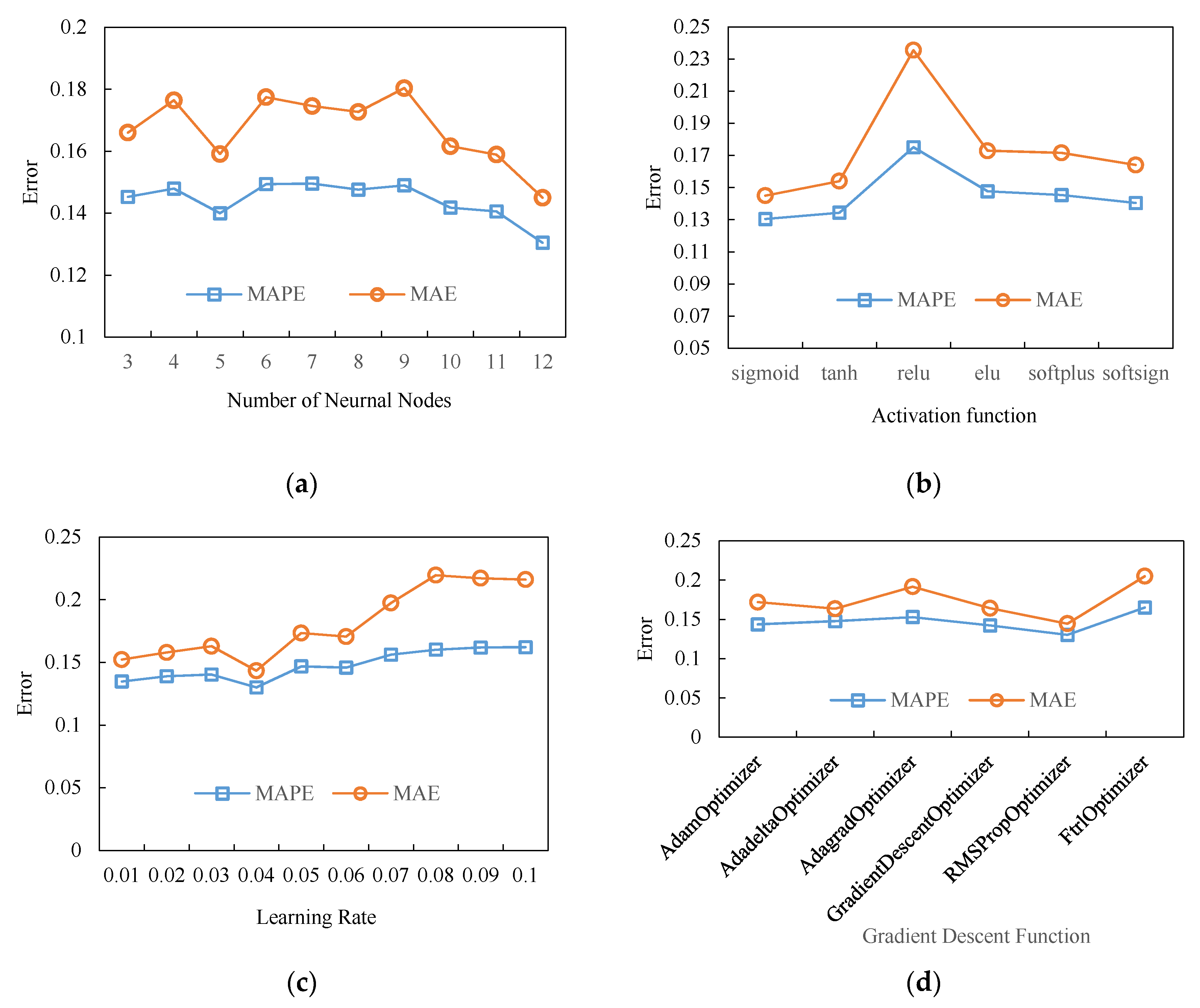
| Number of neural nodes | 12 | 11 | 11 |
| Activate function | sigmoid | sigmoid | Sigmoid |
| Learning rate | 0.04 | 0.06 | 0.04 |
| Gradient descent function | RMSPropOptimizer | AdamOptimizer | AdamOptimizer |
| Model | B 1 | Std. Error 2 | t 3 | Sig. 4 | |
|---|---|---|---|---|---|
| Scenario 1 | Constant | 655.694 | 116.511 | 5.628 | 0.000 |
| PoHV 5 | −96.768 | 16.911 | −5.722 | 0.000 | |
| LW 6 | 243.163 | 35.738 | 6.804 | 0.000 | |
| MTL 7 | −1529.065 | 131.745 | −11.606 | 0.000 | |
| R2 = 0.463 | |||||
| Scenario 2 | Constant | 1969.191 | 209.556 | 9.397 | 0.000 |
| PoHV | −121.196 | 241.416 | −0.502 | 0.617 | |
| PoRV 8 | −1079.966 | 244.811 | −4.411 | 0.000 | |
| Pedestrians | −0.218 | 0.080 | −2.736 | 0.008 | |
| Bicycles | −0.309 | 0.202 | −1.531 | 0.131 | |
| R2 = 0.355 | |||||
| Scenario 3 | Constant | 1617.443 | 87.241 | 18.540 | 0.000 |
| PoLV 9 | −239.322 | 96.053 | −2.492 | 0.016 | |
| Opposing Vehicles | −0.495 | 0.334 | −1.484 | 0.143 | |
| Pedestrians | 0.196 | 0.109 | 1.803 | 0.076 | |
| Bicycles | −0.223 | 0.114 | −1.945 | 0.056 | |
| R2 = 0.170 | |||||
© 2020 by the authors. Licensee MDPI, Basel, Switzerland. This article is an open access article distributed under the terms and conditions of the Creative Commons Attribution (CC BY) license (http://creativecommons.org/licenses/by/4.0/).
Share and Cite
Wang, Y.; Rong, J.; Zhou, C.; Gao, Y. Dynamic Estimation of Saturation Flow Rate at Information-Rich Signalized Intersections. Information 2020, 11, 178. https://doi.org/10.3390/info11040178
Wang Y, Rong J, Zhou C, Gao Y. Dynamic Estimation of Saturation Flow Rate at Information-Rich Signalized Intersections. Information. 2020; 11(4):178. https://doi.org/10.3390/info11040178
Chicago/Turabian StyleWang, Yi, Jian Rong, Chenjing Zhou, and Yacong Gao. 2020. "Dynamic Estimation of Saturation Flow Rate at Information-Rich Signalized Intersections" Information 11, no. 4: 178. https://doi.org/10.3390/info11040178
APA StyleWang, Y., Rong, J., Zhou, C., & Gao, Y. (2020). Dynamic Estimation of Saturation Flow Rate at Information-Rich Signalized Intersections. Information, 11(4), 178. https://doi.org/10.3390/info11040178