Null Models for Formal Contexts †


1
Knowledge & Data Engineering Group, University of Kassel, 34121 Kassel, Germany
2
Interdisciplinary Research Center for Information System Design, University of Kassel, 34121 Kassel, Germany
*
Author to whom correspondence should be addressed.
†
This paper is an extended version of our paper published in the proceedings of the 24th International Conferences on Conceptual Structures, Marburg, Germany, 1–4 July 2019.
‡
These authors contributed equally to this work.
Information 2020, 11(3), 135; https://doi.org/10.3390/info11030135
Submission received: 30 January 2020
/
Revised: 21 February 2020
/
Accepted: 25 February 2020
/
Published: 28 February 2020
(This article belongs to the Special Issue Conceptual Structures 2019)
Abstract
:Null model generation for formal contexts is an important task in the realm of formal concept analysis. These random models are in particular useful for, but not limited to, comparing the performance of algorithms. Nonetheless, a thorough investigation of how to generate null models for formal contexts is absent. Thus we suggest a novel approach using Dirichlet distributions. We recollect and analyze the classical coin-toss model, recapitulate some of its shortcomings and examine its stochastic properties. Building upon this we propose a model which is capable of generating random formal contexts as well as null models for a given input context. Through an experimental evaluation we show that our approach is a significant improvement with respect to the variety of contexts generated. Furthermore, we demonstrate the applicability of our null models with respect to real world datasets.
MSC:
03G10; 68T271. Introduction
This presented work is an extension of the already published conference paper [1]. There we investigated how to randomly generate formal contexts using Dirichlet distributions. Formal contexts are the basic data structure in the realm of formal concept analysis (FCA), a theory used to represent and extract knowledge, which is rooted in lattice theory [2]. These datasets are constituted of a set of objects, a set of attributes and a binary (incidence) relation between them. Many real-world datasets can be interpreted as such formal contexts and are therefore subjected to methods from FCA.
An important problem when investigating datasets through FCA is to decide whether an observation is meaningful or not. Related fields, e.g., graph theory and ecology, employ null model analysis, see [3,4,5]. This method randomizes datasets with the constraint to preserve certain (statistical) properties and can easily be adapted to FCA. Randomly generating formal contexts is also relevant for other applications, e.g., comparing the performance of FCA algorithms, as done in [6,7]. Both applications can be approached by randomly generating formal contexts. Hence, one has to develop (novel) procedures to randomly generate formal contexts. However, known methods for generating adequate random contexts are insufficiently investigated [8] and novel approaches have to be developed.
A naive approach for randomly generating formal contexts is to draw uniformly from the set of all formal contexts on a finite set of attributes M. This approach is infeasible as the number of formal contexts with pairwise distinct objects is . This problem is related to the random generation of Moore families, as investigated in [9]. There, the author suggested an approach to uniformly draw from the set of closure systems for a given set of attributes, which is computationally infeasible for , see [10].
The predominant procedure to randomly generate formal contexts is the coin-toss model, mainly due to the ease of use and the lack of proper alternatives. Yet, this approach is biased to generate a small class of contexts, closely related to the fixed row density contexts, as investigated by Borchmann et al. in [8].
We overcome the so far encountered limitations with a novel approach based on Dirichlet distributions. To this end we first examine the stochastic model of coin-tossing and provide further details explaining the short-comings of this approach. Secondly, we suggest an alternative model to generate formal contexts that addresses some of these short-comings. In particular, we demonstrate how to select appropriate base measures and precision parameters to obtain both random contexts and null models. For this we present a thorough analysis of the influence of these parameters on the resulting contexts. Afterwards we empirically evaluate our model on randomly generated formal contexts with six to ten attributes. We show that our approach is a significant improvement upon the coin-tossing process in terms of the variety of contexts generated. In this extended version, we employ our findings to null model generation for ten real-world formal contexts and four artificially created ones. We identify in there the limitations of our method and propose a possible application for discovering interesting formal contexts.
As for the structure of this paper in Section 2 we first give a short problem description and recall some basic notions from FCA followed by a brief overview of related work in Section 3. We proceed by stochastically modeling and examining the coin-toss and suggest the Dirichlet model in Section 4. In Section 5 we evaluate our model empirically and discuss our findings. In Section 6 we give an introduction to null model analysis in FCA and discuss the applicability of the Dirichlet approach to null model generation. We support the theoretical findings with a study on real-world and artificial contexts. Lastly in Section 7 we give our conclusions and an outlook on future research.
2. FCA Basics and Problem Description
We begin by recalling basic notions from formal concept analysis. For a thorough introduction we refer the reader to [2]. A formal context is a triple of sets. The elements of G are called objects and the elements of M attributes of the context. The set is called incidence relation, meaning the object g has the attribute m. We introduce the common operators, namely the object derivation by , and the attribute derivation by . A formal concept of a formal context is a pair with , such that and . We then call A the extent and B the intent of the concept. With we denote the set of all concepts of some context . A pseudo-intent of is a subset where and holds for every pseudo-intent . In the following we may omit formal when referring to formal contexts and formal concepts. Of particular interest in the following is the class of formal contexts called contranominal scales. These contexts are constituted by where . The number of concepts for a contranominal scale with n attributes is , thus having intents and therefore zero pseudo-intents. If a context fulfills the property that for every there exists an object such that , then contains a subcontext isomorphic to a contranominal scale of size , i.e, such that with .
In this paper we deal with the problem of randomly generating a formal context given a set of attributes. Our motivation originates in Figure 1 where we show 5000 randomly generated contexts with ten attributes. The model used to generate these contexts is a coin-toss, as recalled more formally in Section 4. This method is the predominant approach to randomly generate formal contexts. In Figure 1 we plotted the number of intents versus the number of pseudo-intents for each generated context and a histogram counting occurrences of pseudo-intents. We may call this particular plotting method I-PI plot, where every point represents a particular combination of intent number and pseudo-intent number, called I-PI coordinate. Note that having the same I-PI coordinate does not imply that the corresponding contexts are isomorphic. However, different I-PI coordinates imply non-isomorphic formal contexts. The reason for employing intents and pseudo-intents is that they correspond to two fundamental features of formal contexts, namely concept lattice and canonical implication base, which we will not introduce in the realm of this work.
We observe in Figure 1 that there appears to be a relation between the number of intents and the number of pseudo-intents. This was first mentioned in a paper by Borchmann [11]. Naturally, the question emerges whether this empirically observed correlation is based on a structural connection between intents and pseudo-intents rather than chance. As it turned out in a later study this apparent correlation is most likely the result of a systematic bias in the underlying random generation process [8].
We therefore strive after a novel approach that does not exhibit this or any other bias. Consistently with the above the I-PI coordinates and their distribution are used as an indicator for how diverse created contexts are. The coin-toss approach will serve as a baseline for this. We start by analyzing the coin-toss model which leads to a formalization fitted to the requirements of FCA in Section 4. This enables us to discover Dirichlet distributions as a natural generalization.
3. Related Work
The problem depicted in Section 2 gained not much attention in the literature so far. The first observation of the correlation between the number of intents and pseudo-intents in randomly generated contexts was by Borchmann as a side note in [11]. The phenomenon was further investigated in [8] with the conclusion that it is most likely a result of the random generation process. Their findings suggest that the coin tossing approach as basis for benchmarking algorithms is not a viable option and other ways need to be explored. Related to this is a work by Ganter on random contexts in [9]. There the author looked at a method to generate closure systems in a uniform fashion, using an elegant and conceptually simple acceptance-rejection model. However, this method is infeasible for practical use. Furthermore, the authors in [12] developed a synthetic formal context generator that employs a density measure. This generator is composed of multiple algorithms for different stages of the generation process, i.e., initialization to reach minimum density, regular filling and filling close to the maximum density. However, the survey in [8] found that the generated contexts exhibited a different type of systematic bias.
4. Stochastic Modelling
In the following we analyze and formalize a stochastic model for the coin-toss approach. By this we unravel crucial points for improving the random generation process. To enhance the readability we write to denote that Z is both a random variable following a certain Distribution and a realization of said random variable.
4.1. Coin-Toss—Direct Model
Given a set of attributes M we construct utilizing a direct coin-toss model as follows. We let G be a set of objects with and draw a probability . For every we flip a binary coin denoted by , i.e., where and , and let if and if . Then we obtain the incidence relation by . Hence, I contains all those where the coin flip was a success, i.e., . If we partition the set of coin-tosses through grouping, i.e., , and look for some object g at the number of successful tosses, we see that they follow a distribution. In detail, a binomial distribution with trials and a success probability of p in each trial. This means that no matter how G, M and the probability p are chosen, we always end up with a context where the number of attributes per object is the realization of a distributed random variable for every object .
Example 1.
We generated 5000 contexts with the coin-tossing approach. A plot of their I-PI coordinates and a histogram showing the distribution of pseudo-intents are shown in Figure 1. In the histogram we omitted the high value for zero pseudo-intents. This value emerges from the large amount of generated contranominal scales by the coin-toss model. In particular, 1714 of the contexts contain a contranominal scale and have therefore zero pseudo-intents.
We observe that most of the contexts have less than 100 pseudo-intents with varying numbers of intents between 1 and 1024. The majority of contexts has an I-PI coordinate close to an imaginary curve and the rest has, in most cases, less pseudo-intents, i.e., their I-PI coordinates lie below this curve. Looking at the histogram we observe a varying number of pseudo-intents. We have a peak at zero and a high number of 126 contexts with one pseudo-intent. Additionally there is a peak of 62 contexts with 36 pseudo-intents and a peak of 55 contexts with 73 pseudo-intents. In between we have a low between 18 to 23 pseudo-intents and one around 50.
4.2. Coin-Toss: Indirect Model
In order to exhibit a critical point in the direct coin-tossing model we introduce an equivalent model using an indirect approach, called indirect coin-toss. Furthermore, this model serves as an intermediate stage to our proposed generation scheme.
As we just established, the number of successful coin-tosses, i.e., number of attributes per object, follows a binomial distribution. An indirect model that generates the same kind of formal contexts as direct coin-tossing can therefore be obtained by using a binomial distribution. In contrast to the direct model we first determine the total number of successful coin-tosses per object and pick the specific attributes afterwards. We formalize this model as follows.
Given a set of attributes M, as before, we let G be a set of objects with and draw a probability . For every we let be the number of attributes associated to that object g. Hence, . We let be the set of all possible attribute combinations for g and denote by the discrete uniform distribution on . Now for every we let to obtain the set of attributes belonging to the object g and define the incidence relation by . This serves as a foundation for our proposed generation algorithm in Section 4.3. The indirect formulation reveals that the coin tossing approach is restricting the class of possible distributions for , i.e., the number of attributes for the object g, to only the set of binomial ones. Thereby it introduces a systematic bias as to which contexts are being generated. An example for a context that is unlikely to be created by the coin-tossing model is a context with ten attributes where every object has either two or seven attributes.
4.3. Dirichlet Model
One way to improve the generating process is to use a broader class of discrete distributions to determine . In the indirect coin-tossing model we were drawing from the class of binomial distributions with a fixed number of trials. In contrast to that we now draw from the class of all discrete probability distributions on the same sample space, i.e., distributions that have the same support of , which in our case represents the possible numbers of attributes for an object. For finite sample spaces every probability distribution can be considered as a categorical distribution. Therefore, a common method to draw from the class of all discrete probability distributions is to employ a Dirichlet distribution. In Bayesian statistics this distribution is often utilized as prior distribution of parameters of a categorical or multinomial distribution [13].
One way to define the Dirichlet distribution is to use gamma distributions [13]. A distribution with shape parameter and scale parameter can be characterized on the real line with respect to the Lebesgue measure by a density function if , where denotes the indicator function on some set S and denotes the gamma function. In the case of the gamma distribution degenerates at zero. The distribution with parameters , where , for all i and for some and , is a probability distribution on the set of K-dimensional discrete distributions. Given independent random variables with it is defined as the distribution of a random vector where for . Note that this allows for some of the variables to be degenerate at zero which will be useful in the application for null models, as we will describe in Section 6. If for all i the random vector has a density
on the simplex . Note that f in Equation (1) is a density with respect to the -dimensional Lebesgue measure and we can rewrite f as a -dimensional function by letting and using an appropriate simplex representation. Moreover, note that the elements of have the expected value , the variance and the co-variance for . Hence, the parameter is called base measure or mean as it describes the expected value of the probability distribution and is called precision parameter and describes the variance of probability distributions with regard to the base measure. A large value for will cause the drawn distributions to be close to the base measure, a small value will cause them to be distant. A realization of a Dirichlet distributed random variable is an element of S and can therefore be seen as probability vector of a K-dimensional categorical distribution.
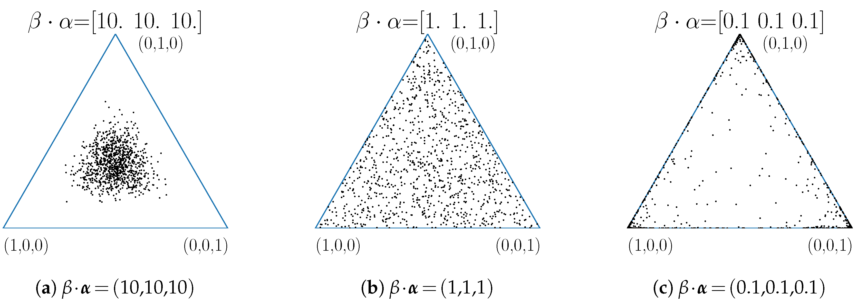
In Figure 2 we illustrate the effects of varying . We show different distributions of probabilities for three categories drawn from 3-dimensional Dirichlet distributions. The base measure in each case is the uniform distribution, i.e., , the precision parameter varies. The choice of then results in a uniform distribution on the probability simplex. For comparison we also chose and . A possible interpretation of the introduced simplex is the following. Each corner of the simplex can be thought of as one category. The closer a point in the simplex is to a corner the more likely this category is to be drawn.
In the rest of this section we describe the model for our proposed random formal context generator. Given a set of attributes M, we let G be a set of objects with . We then use a probability vector to determine the probabilities for an object to have 0 to attributes, where with . By using as base measure and , which implies , we draw uniformly from the set of discrete probability distributions. As a different way to determine we can therefore use as probabilities of a dimensional categorical distribution . These categories are the numbers of attributes for an object, i.e., for . Looking back at Section 4.2 we replace the binomial distribution based on a uniformly distributed random variable by a categorical distribution based on a Dirichlet distributed one. Afterwards we proceed as before. We present pseudocode for the Dirichlet approach in Algorithm 1 as a further reference for the experiments in Section 5.
| Algorithm 1: Dirichlet Approach |
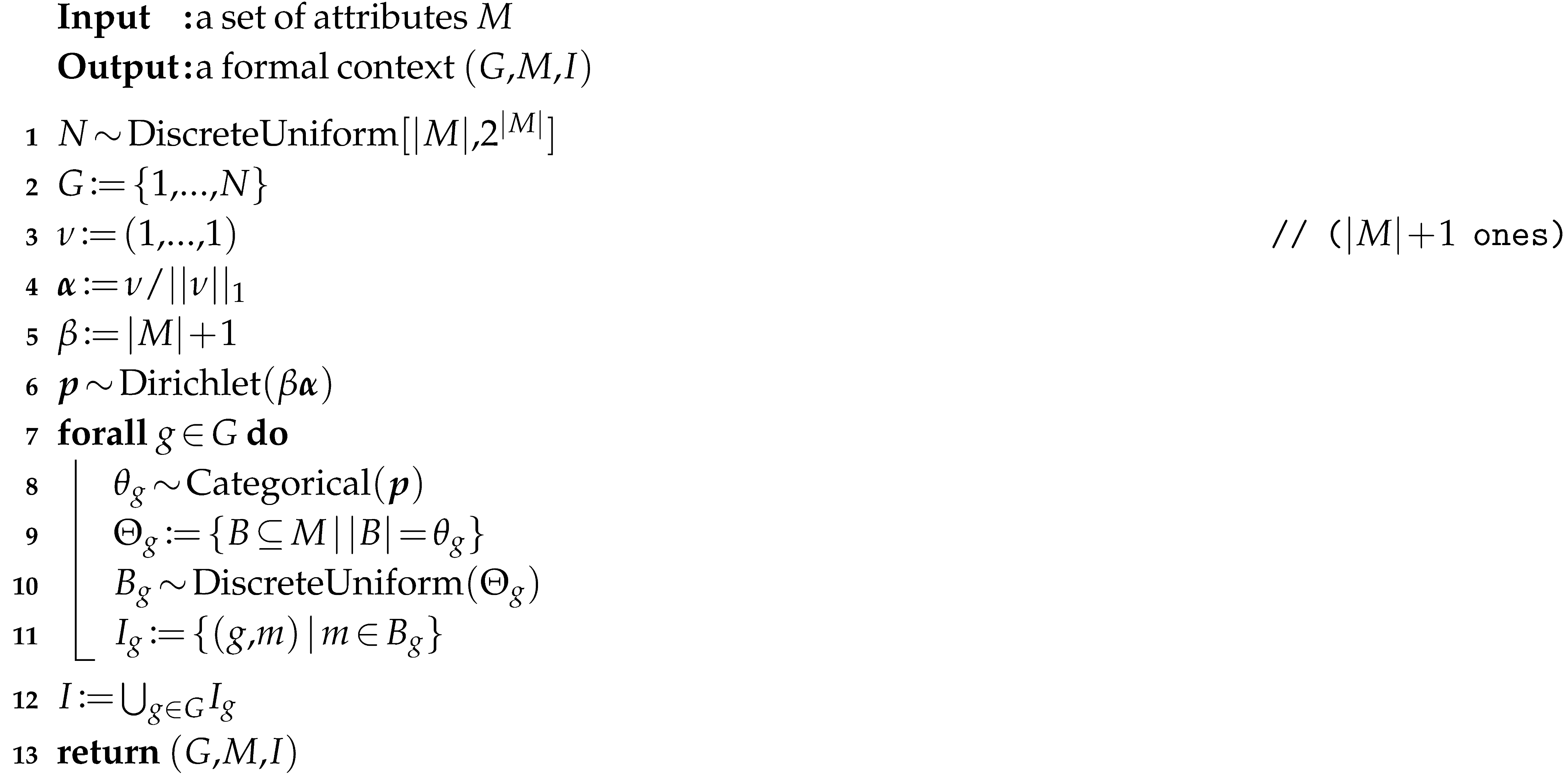 |
5. Experiments
In this section we present a first experimental investigation of Algorithm 1. We evaluated the results by examining the numbers of intents and pseudo-intents of generated contexts. The contexts were generated using Python 3 and all further computations, i.e., the I-PI coordinates, were done using conexp-clj [14]. The generator code as well as the generated contexts can be found on GitHub (Online Repository containing Data, Results, Code: https://github.com/maximilian-felde/formal-context-generator).
5.1. Observations
For each experiment we generated 5000 formal contexts with an attribute set M of ten attributes using Algorithm 1. We also employed slightly altered versions of this algorithm. Those alterations are concerned with the choice of , as we will see in the following. We plotted the resulting I-PI coordinates and a histogram of the pseudo-intents for each experiment. In the histogram we omitted the value for zero pseudo-intents, i.e., the peak for contexts containing a contranominal scale of size . A comparable experiment on ten attributes is described in Example 1, where a (direct) coin-toss model was utilized. The results of Example 1 are shown in Figure 1. This will serve as a baseline in terms of variety and distribution of I-PI coordinates.
First we used Algorithm 1 without alterations. The results are depicted in Figure 3. We can see that most of the generated contexts have less than 75 pseudo-intents and the number of intents varies between 1 and 1024. There is a tendency towards contexts with fewer pseudo-intents and we cannot observe any context with more than 101 pseudo-intents. The number of generated contexts containing contranominal scales of size was 2438. The histogram shows that the number of contexts that have a certain quantity of pseudo-intents decreases as the number of pseudo-intents increases with no significant dips or peaks. In this form the Dirichlet approach does not appear to be an improvement over the coin-tossing method. In contrary, we observe the spread of the number of pseudo-intents to be smaller than in Example 1.
Our next experiment was randomizing the precision parameter between 0 and , i.e., let in Algorithm 1, Line 5. We will refer to this alteration as variation A. The results are shown in Figure 4. We can see that again many contexts have less than 100 pseudo-intents and the number of intents once again varies over the full possible range. There are 1909 contexts that contain a contranominal scale of size . However, we notice that there is a not negligible number of contexts with over 100 and up to almost 252 pseudo-intents, which constitutes theoretical maximum [8]. Most of these gather around nearly vertical lines close to 75, 200, 380, 600 and 820 intents. Even though most of the contexts have an I-PI coordinate along one of those lines there are a few contexts in-between 100 and 175 pseudo-intents that do not fit this description. Looking at the histogram we can observe again that while the number of pseudo-intents increases the number of generated contexts to that pseudo-intent number decreases. This is in contrast to Example 1. This time, however, we can clearly see a peak at seven to ten pseudo-intents with 190 contexts having ten pseudo-intents. Apart from this we observed no other significant dips or peaks. We also tried randomizing the base measure using Dirichlet distributions. However, this did not improve the results.
Since the last experiment revealed that small values for resulted in a larger variety of contexts we will now investigate those in more detail. For this we introduce a constant factor c such that . We find for the experiment called variation B the factor suitable, as we will explain in Section 5.2. A plot of the results can be found in Figure 5. We can see that most of the contexts have less than 150 pseudo-intents and the number of intents is between 1 and 1024. Furthermore, the quantity of contexts containing a contranominal scale of size is 1169. This number is about 700 lower than in variation A, roughly 500 lower compared to the coin-tossing results in Example 1, and over 1200 lower than in the unaltered Dirichlet approach. We can again observe the same imaginary lines as mentioned for variation A, with even more contrast. Finally, we observe that the space between these lines contains significantly more I-PI coordinates. Choosing even smaller values for c may result in less desirable sets of contexts. In particular, we found that lower values for c appear to increase the bias towards the imaginary lines.
The histogram (Figure 5) of variation B differs distinguishably to the one in Figure 4. The distribution of pseudo-intent numbers is more volatile and more evenly distributed. There is a first peak of 366 contexts with ten pseudo-intents, followed by a dip to eleven contexts with seventeen pseudo-intents and more relative peaks of 50 to 60 contexts each at 28, 36 and 45 pseudo-intents. After 62 pseudo-intents the number of contexts having this amount of pseudo-intents or more declines with the exception of the peak at 120 pseudo-intents.
We established that both variations of Algorithm 1 with and are improvements upon the coin-tossing approach. In order to further increase the confidence in our Dirichlet approach we have generated 100,000 contexts with the coin-tossing approach as well as with both variations for six, seven and eight attributes. We compared the distinct I-PI coordinates after certain numbers of generated contexts. The results of this experiment is shown in Figure 6. Each subfigure shows the results for one attribute set size. We have plotted the number of generated contexts versus the number of distinct I-PI coordinates for the coin-toss (green solid line), variation A (orange dashed line) and variation B (blue dotted line). In all three plots we recognize that there is a steep increase of distinct I-PI coordinates at the beginning followed by a fast decline in new I-PI coordinates, i.e., a slow increase in the total number of distinct I-PI coordinates, for all three random generation methods. The graphs remind of sublinear growth. For all three attribute set sizes we can observe that the graphs of variation A and B lie above the graph of the coin-toss. Hence, variation A and B generated more distinct contexts compared to the coin-toss. Exemplary for the coin-tossing approach resulted in 1963 distinct I-PI coordinates and reached them after around 99,000 generated contexts. Variation A generated around 19,000 contexts until it hit 1963 distinct I-PI coordinates and reached a total of around 2450 after 100,000 contexts generated. Variation B reached the same number of distinct I-PI values already at around 13,000 generated contexts and resulted in 2550 distinct I-PI coordinates.
5.2. Discussion
We begin the discussion by relating the parameters of the Dirichlet approach to the variety of generated contexts. Afterwards we explore the discrepancy in the quantities of contexts that contain a contranominal scale and discuss the observed imaginary lines. Lastly, we discuss the ability of the different approaches for generating pairwise distinct I-PI coordinates efficiently.
The Dirichlet approach has two parameters, one being the parameter related to the variance of the Dirichlet distribution, the other being the parameter which describes the expected value of the Dirichlet distribution, as explained more formally in Section 4.3. A large value for results in categorical distributions that have probability vectors close to the base measure , following from the definition. A small value for results in categorical distributions where the probability vectors are close to the corners or edges of the simplex, see Figure 2c. As already pointed out in Section 4.3, those corners of the simplex can be thought of as the categories, i.e., the possible numbers of attributes an object can have. This implies that for large the categories are expected to be about as likely as the corresponding probabilities in the base measure. Whereas, for small one or few particular categories are expected to be far more likely than others.
We have seen that the Dirichlet approach without alterations generated around 2450 contexts containing a contranominal scale of size . This number was 1900 for variation A and 1200 for variation B. One reason for the huge number of contranominal scales generated by the base version of the Dirichlet approach is that most of the realizations of the Dirichlet distribution (Algorithm 1, Line 6) are inner points of the probability simplex, i.e., they lie near the center of the simplex. These points or probability vectors result in almost balanced categorical distributions (Algorithm 1, Line 8), i.e., every category is drawn at least a few times for a fixed number of draws. This fact may explain the frequent occurrence of contranominal scales. The expected number of objects with attributes that need to be generated for a context to contain a contranominal scale is low. In more detail, we only need to hit the equally likely distinct objects, having attributes during the generation process. To be more precise, the mean and the standard deviation of the number of required objects with attributes can easily be computed via and with , cf. [15], as this is an instance of the so-called Coupon Collector Problem. For example for a context with ten attributes we get and , hence we need to generate on average around 30 objects with nine attributes to create a contranominal scale. While, there is already a high probability of obtaining a contranominal scale after generating around 18 objects. This means if we generate a context with objects and the probability for the category with nine attributes is around we can expect the context to contain a contranominal scale.
If we use a lower value for we tend to get less balanced probability vectors from the Dirichlet distribution and therefore generate less contexts that contain a contranominal scale. The pathological case is a close to zero, which leads to contexts where all or nearly all objects have the same number of attributes. Even then we could expect at least of the contexts generated to contain a contranominal scale. In this case we basically draw from the set of categories, i.e., from the possible numbers of attributes. Those are related as corners of the simplex and the probability to land in the corner belonging to the category of attributes is approximately .
Contexts where every object has the same number of attributes are referred to as contexts with fixed row-density in [8]. They were used to show that the coin-tossing approach in practice does not generate a whole class of contexts. An explanation for the imaginary lines observed in Figure 4 and Figure 5 is that they correspond to contexts with fixed row-density, cf. ([8] Figure 5). As pointed out in the last paragraph very low values of the Dirichlet approach predominantly generates contexts where all objects belong to few or even only one category. This explanation is further supported by the increasing bias of the context’s I-PI coordinates to form those imaginary lines for decreasing values of . It also accounts for the peak at ten pseudo-intents in the histograms for variations A and B. This due to the fact that a fixed row-density context with density that contains all possible objects has exactly ten pseudo-intents, cf. ([8] Prop. 1). This is again related to the Coupon Collector Problem. The solution to this problem yields the expected number of objects that we need in order to hit every possible combination. In particular for the case of the peak at ten pseudo-intents, , and , meaning if we generate a fixed row-density context with around 200 objects we can expect it to contain all possible combinations and therefore have ten pseudo-intents. This fits well with the observed 366 contexts with ten pseudo-intents in variation B. Consider the case that we only generate fixed row-density contexts containing all possible attribute combinations and all densities are equally likely. The expected number of contexts with eight attributes and therefore ten pseudo-intents for 5000 generated contexts then is . Naturally, variation B does not predominantly generate fixed row-density contexts or even fixed row-density contexts with all possible attribute combinations. Hence, the before mentioned 366 observed contexts with ten pseudo-intents seem reasonable.
Lastly we discuss the observations from counting distinct I-PI coordinates. In Figure 6 we can see that the Dirichlet approach results in a broader variety of contexts in comparison to the coin-tossing for any fixed number of generated contexts. All three plots show that there is an initial phase where contexts with new I-PI coordinates are frequently generated followed by a far longer part where contexts with new I-PI coordinates become increasingly rare. This is not surprising, since the number of possible I-PI coordinates is finite and the probability to re-hit increases with every distinct generated I-PI coordinate. Note that this is an effect that would also be observed when using a perfectly uniform sampling mechanism. Nonetheless, what we can observe is that it takes the Dirichlet approach significantly longer, compared to the coin-tossing model, to reach a point where only few new I-PI coordinates are generated.
5.3. The Problem with Contranominal Scales
In the previous part of the discussion we established that contranominal scales pose a serious problem while generating formal contexts. In particular when a formal context contains large or the largest possible contranominal scale. One possible way to prevent this is to set the probability to generate objects with attributes to zero while generating formal contexts with attributes. This results in the impossibility of generating a contranominal scale of size . However, this would diminish the class of generable contexts significantly. A more sophisticated approach to alter the precision parameter and the base measure would consider more specific classes of those. Nonetheless, the research for understanding the influence of the base measure and the precision parameter is in its beginning with respect to context generation. Hence, we encourage a detailed investigation of this in future work. Until then, using the base measure that results in a uniform draw of the categorical distribution and randomizing the precision parameter is a good trade-off. For dealing with an already generated contranominal scale of size we propose the following course of action. The approach at hand is to discard this particular context and to generate a new one. A more advanced method is to remove all instances of at least one attribute combination on attributes. Furthermore, detecting and removing a contranominal scales of lesser size is possible but computationally infeasible.
6. Applications
We see for our Dirichlet approach at least two major applications. For one, an improved random generation process can be used to facilitate more reliable benchmarks for FCA algorithms. For example, since the Dirichlet approach generates contexts that exhibit a greater variety, i.e., a larger class of generated contexts compared to coin-tossing, it can be used to obtain more robust runtime results. A second application is the generation of null models for formal contexts. In a nutshell, the idea of null model analysis for formal contexts is to obtain information about a context of interest by comparing it to similar, randomly generated contexts. Similar means here that the random contexts mimic some properties of the original context either precisely or approximately.
6.1. Null Models for Formal Contexts
We start with a quick recollection of graph theoretic null models. Thereafter, we introduce null models for formal contexts and their generation using our Dirichlet approach. We conduct an experimental comparison of coin-toss and the Dirichlet generator for their ability to mimic real-world contexts as well as randomly generated ones. Afterwards, we conclude this investigation with an application for deciding the interestingness of a formal context.
In graph theory null models are well employed, c.f. [3,16,17], and one prominent use-case is community detection in graphs by Newman [18]. There the graph of interest is compared to instances of the graph with randomized edges (under certain constraints) to determine its community structure. Essentially, the graph of interest is compared to random graphs that have the same number of nodes and the same node degree distribution. An extension to this null model incorporates expected degree distributions [19] and is able to capture certain peculiarities arising from real-world graphs more robustly. Note that using the exact or expected node degree distributions are just two of many possibilities to specify a null model. Other (graph) null models, for example, are based on the Bernoulli (Erdösh–Reni) random graphs, the Barabasi–Albert graph model, the Watts–Strogatz graph model or other task specific random approaches. Adapting the expected node degree distribution model allows us to develop a Dirichlet based null model for formal contexts.
The graph based idea of null models can easily be transferred to formal contexts. It is known that for every formal context a bipartite graph can be constructed in the following way: The vertex set is constituted by the disjoint union of the object set and the attribute set. The set of edges is constructed from the incidence relation in a natural way, i.e., an object and an attribute that are related in the context have an edge between the corresponding vertices in the graph. Analogously, a formal context can be constructed from a bipartite graph by using the partitions as objects and attributes and the edges to determine the incidence relation.
Assume now we have a formal context and we want to construct a null model for . We then interpret as bipartite graph and construct a graph based null model. The resulting (null model) graphs are then re-interpreted as formal contexts and constitute the null model for . This being said, algorithmically we omit the explicit transformations and conduct the graph based null model generation on the formal context side directly. For our investigation we examine Newman’s null model [18]. This model preserves the node degree distribution of a bipartite graph. This translates to the preservation of the number of incidences for each object and for each attribute in the formal context. Hence, a randomization technique that can be used to imitate Newman’s null model directly on formal contexts is swapping of incidences (SWAP). This means we repeatedly select two objects and two attributes such that if and we swap their incidences such that and . This generates a randomized version of the original context under the constraint to preserve the node degree distribution. However, this technique is obviously a frail randomization approach due to the constraint for swapping.
Considering only one partition element of a bipartite graph for the null model generation is still a reasonable endeavor. This idea translates to focusing on either the attribute set or the object set in a formal context. From this a less restrictive null model can then be derived. This model is less restrictive with respect to the SWAP approach, since structural properties are only kept for either the object set or the attribute set. For example, only the degree distribution of the object set is preserved. Building up on this we focus in the following, without loss of generality, on the object set. More specifically we consider the number of attributes per object, also referred to as row sums. This corresponds very well to our model for randomly generating formal contexts, cf. Section 4.3. Note that the row sums in a formal context correspond to the node degrees of the objects in the corresponding bipartite graph. Therefore, the row sum distribution of a formal context is the same as the object node degree distribution in the corresponding bipartite graph. An example for a row sum preserving null model for a formal context is derived as follows. For all objects permute the incidence with the attribute set in the original context. This clearly leaves the row sum of every object intact. Hence, the row sum distribution of the altered context is equal to the distribution in the original context.
The last generalization before discussing our novel Dirichlet based null model is the following idea. Instead of preserving the row sum distribution one may retreat to preserve this only to some approximation. For example, one may employ the observed row sum distribution from the original formal context as prior for a categorical distribution. Here, the categories reflect the number of attributes. For example, if has ten attributes then each to be sampled object can have between zero and ten attributes. These are the categories of the distribution and the corresponding probabilities are the relative frequencies of their occurrence in . To generate a new random context from this distribution we then draw for each object from a new number of attributes and draw accordingly many elements from the attribute set c.f. Algorithm 1 lines 8 to 11. This procedure does not necessarily preserve the row sum distribution, but the expected distribution is equal to the distribution of the original context.
The Dirichlet Null Model for Formal Contexts
Our novel approach for null model generation is closely related to the model discussed above. However, we additionally introduce small deviations from the original row sum distribution. To this end we employ the normalized row sum distribution of as a base measure for the Dirichlet distribution. We may note that this requires the ability to deal with zero components in the base measure, as mentioned in Section 4.3. Furthermore, a large value for the precision parameter is necessary to control the deviation from the original row sum distribution. The expected row sum distribution in our approach resembles the distribution in the original context.
For obvious reasons this null model can be computed using the Dirichlet random generator as introduced in Section 4.3. Explicitly, for one may apply Algorithm 1 with in Line 1, the row sum distribution from as in Line 4 and a large value for , e.g., , in Line 5.
An overview for the so far introduced gradations of formal context null models is depicted in Table 1. We added additionally a simple resampling approach (last line).
6.2. Evaluation of the Dirichlet Approach for Null Model Generation
We evaluate in this section our approach for null model generation. To this end, we use Algorithm 1 with the alterations specified in the last section. Namely, for some context we use its row sum distribution as base measure , the number of attributes as N and a high precision parameter . In addition to the discussed Dirichlet null model we employ resampling as a base line null model. That is, we generate random contexts by sampling objects from the original context. Furthermore we compare our null model approach to the classical coin-toss procedure, i.e., we generate random contexts using the coin-toss algorithm where the coin is weighted with respect to the original context.
Altogether we investigate a set of ten real-world contexts and four artificial contexts for our evaluation. The evaluation set is diverse. Nonetheless, with respect to the number of attributes we had to select formal contexts where the computation of the intent set and and pseudo-intent set is computationally feasible. The set of contexts as well as the code used for the evaluation can be found online, see Section 5 on page 7 and the datasets of the conexp-clj software [14]. Short summaries of the used contexts and their properties are depicted in Table 2 and Table 3.
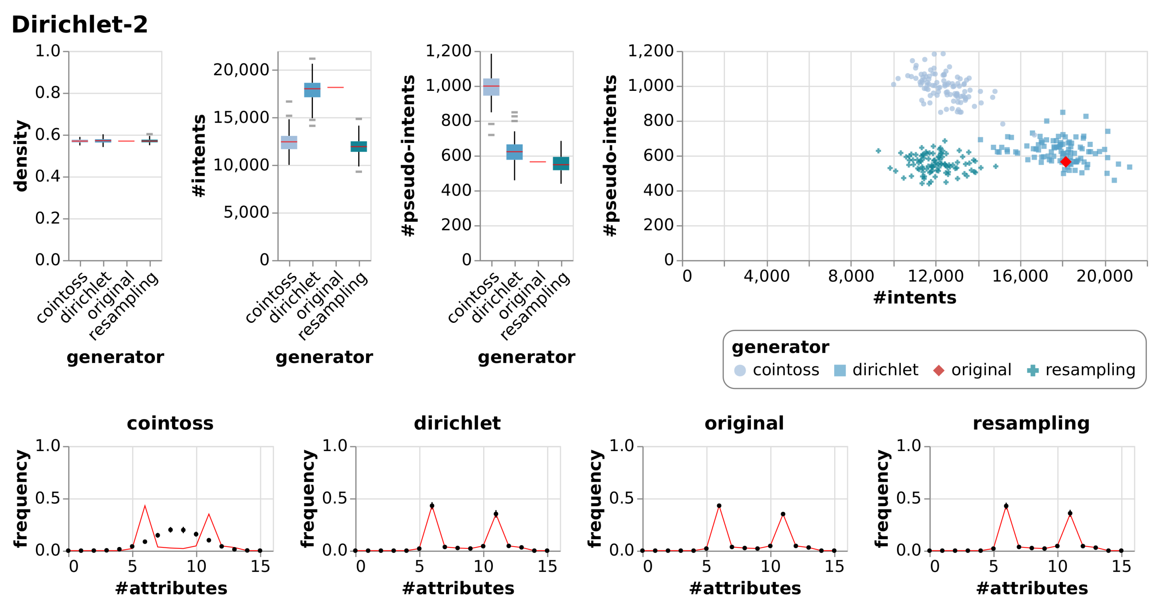
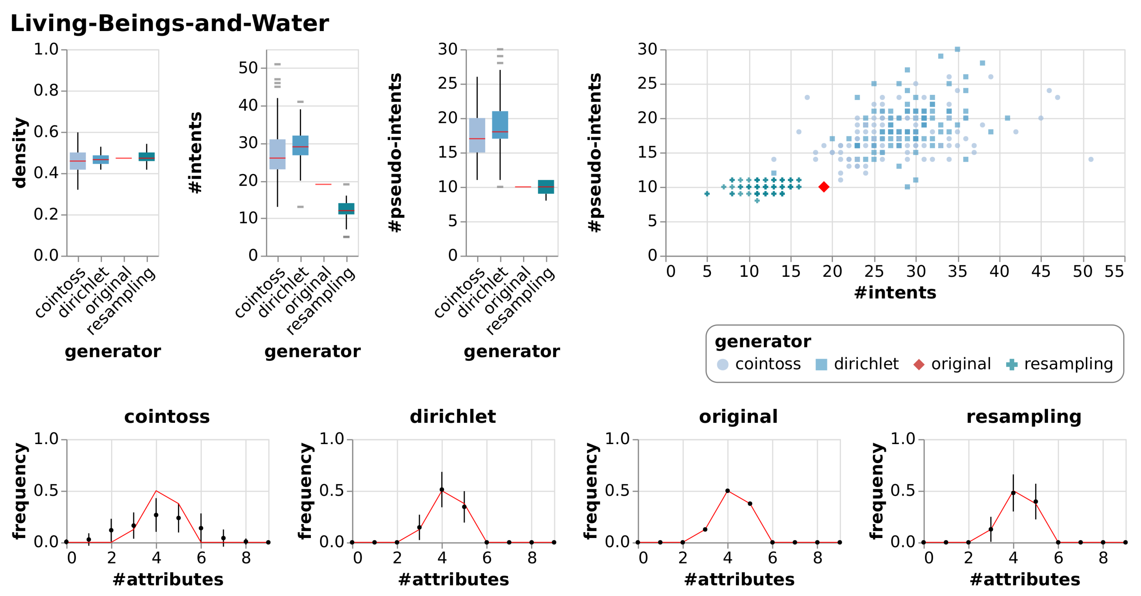
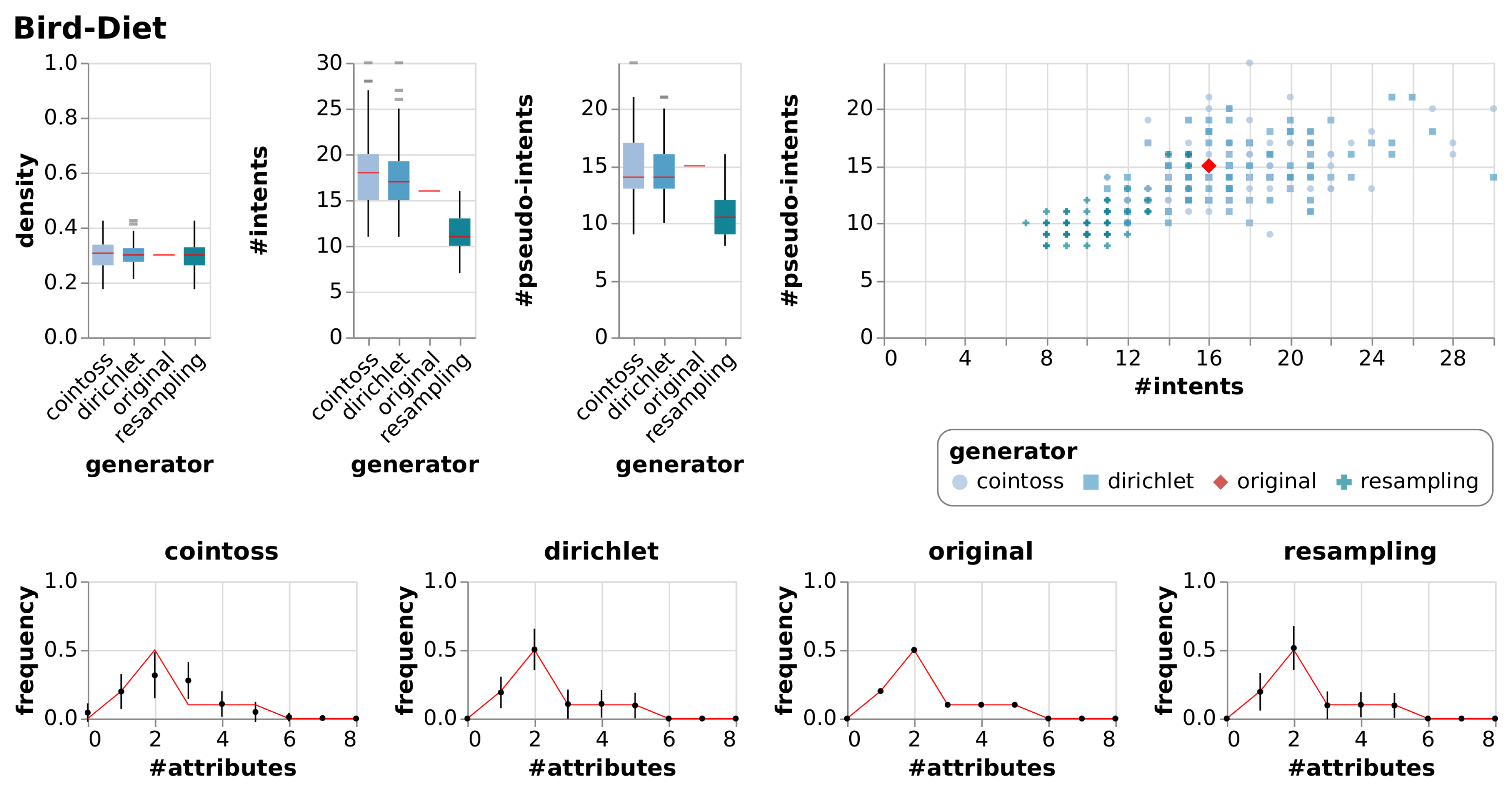
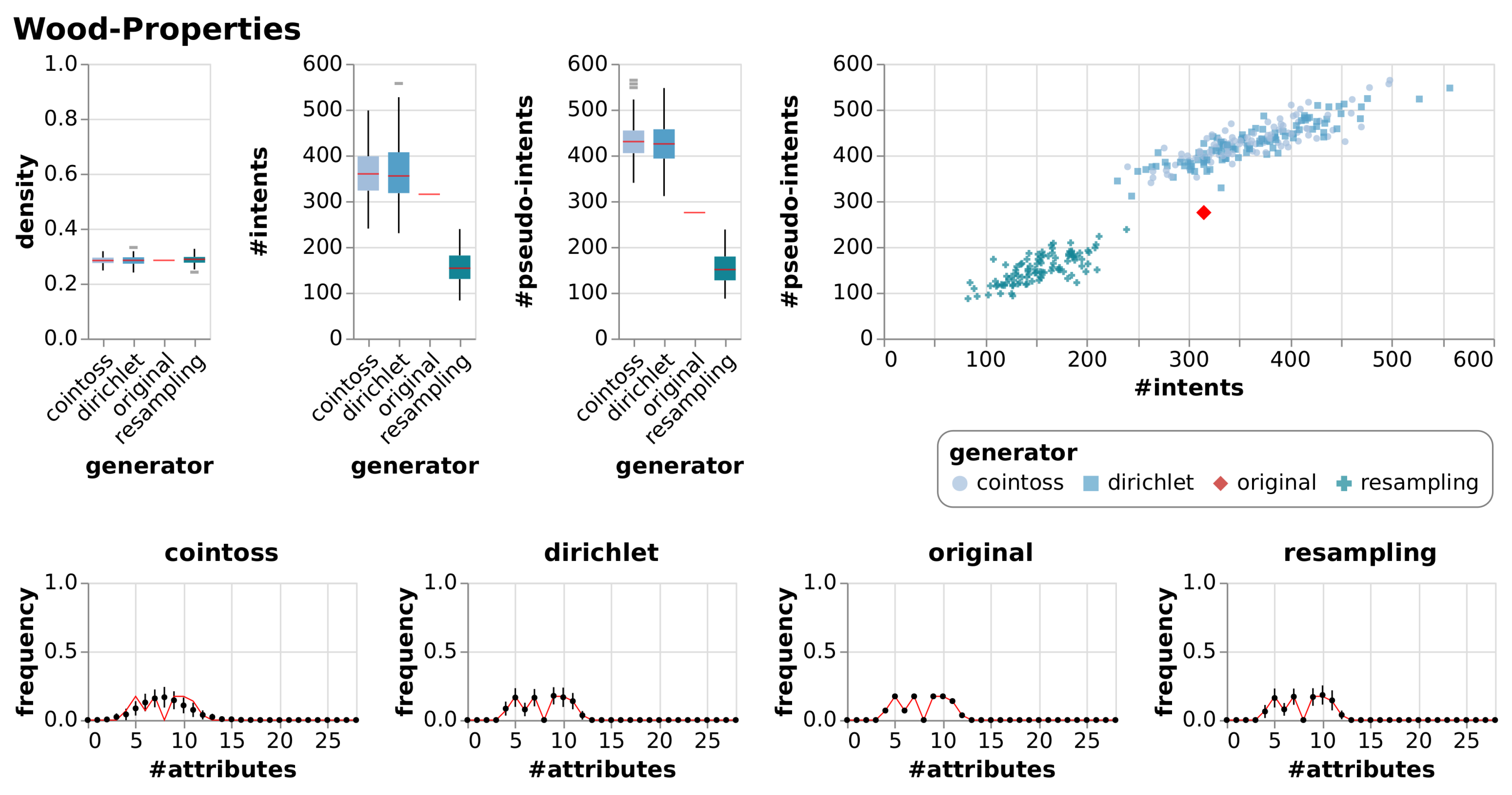
For the evaluation of our Dirichlet approach for null models we generated one null model per context per approach (Dirichlet, coin-toss, resampling). Each null model consists of 100 randomly generated formal contexts based on the properties of the original contexts. All generated contexts have the same number of attributes and the same number of objects as the original contexts. We have computed the density, the number of intents and the number of pseudo-intents for all generated contexts and aggregated them for each null model in Table 3. Note that all non-integer values have been rounded to two decimal places. Furthermore, we have prepared visual representations of the results for all contexts, from which we only included a selection in the main matter of this work. More specifically, we present the results for three real-world contexts and one artificial context. The remaining visualizations can be found in the appendix (Figure A1, Figure A2, Figure A3, Figure A4, Figure A5, Figure A6, Figure A7, Figure A8, Figure A9 and Figure A10). The first graphic (Figure 7) contains a detailed description of the shown plots.
6.2.1. Observations
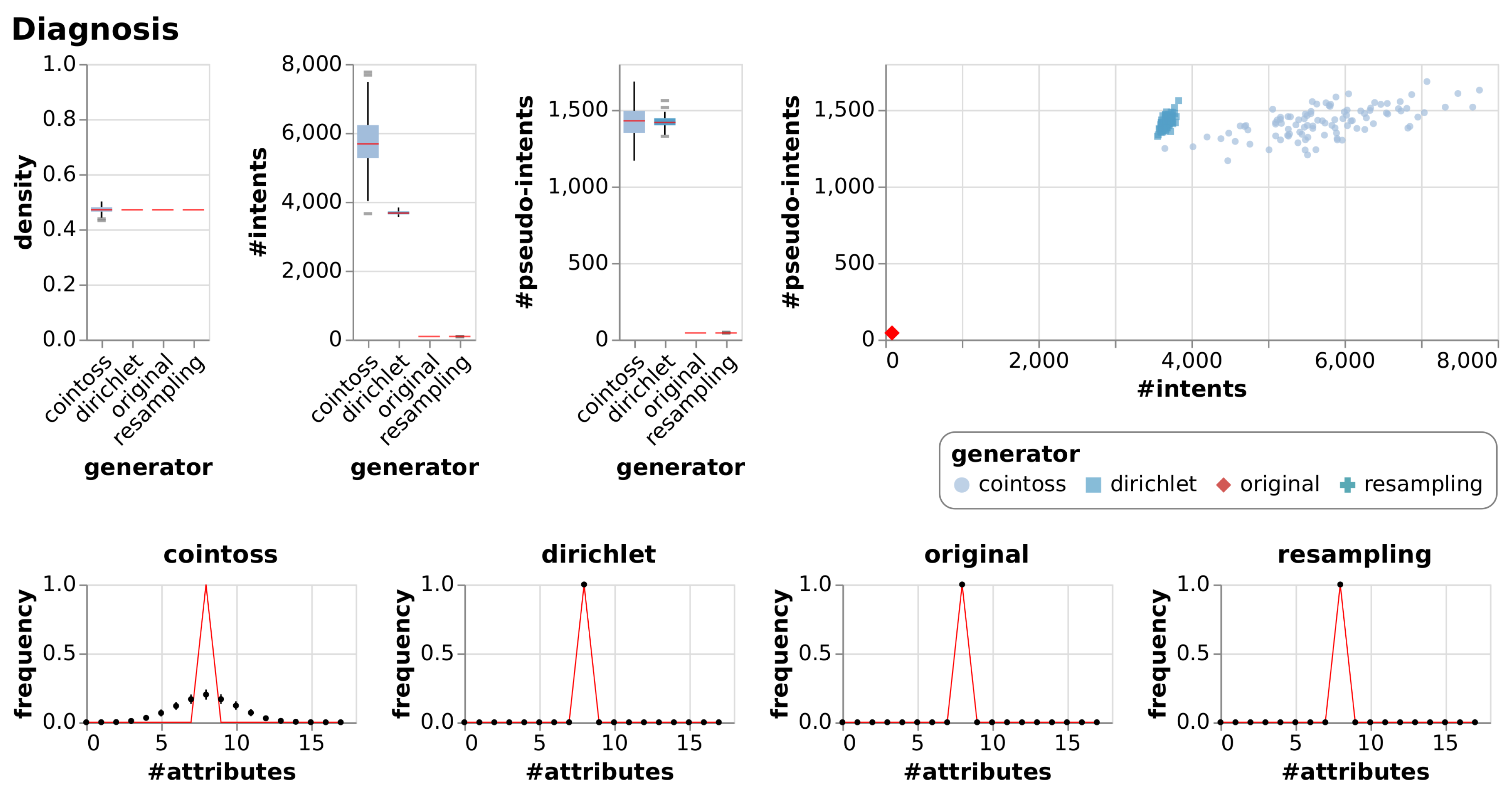
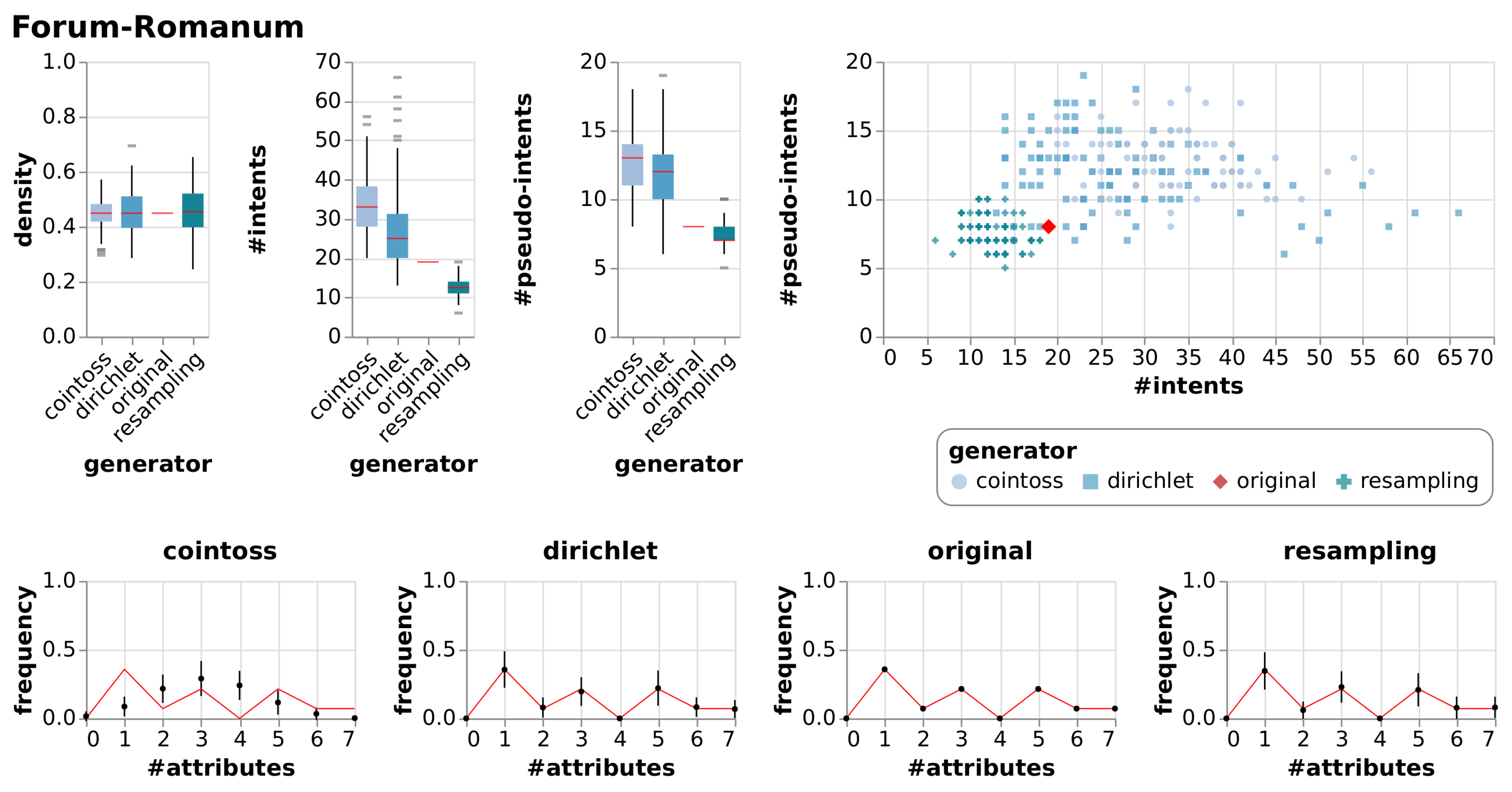
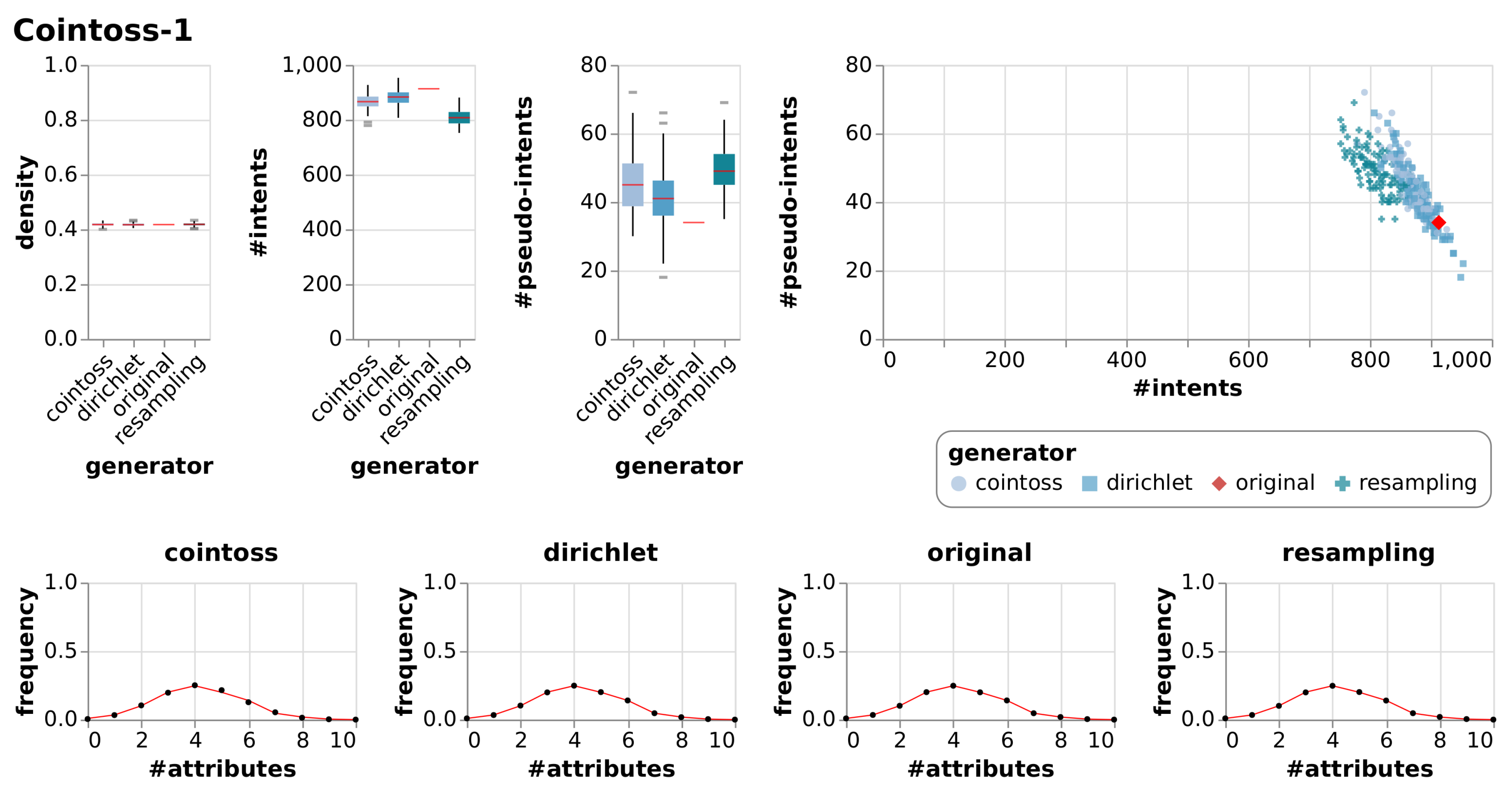
In addition to the visualizations in Figure 7, Figure 8, Figure 9 and Figure 10 we summarized the result in a numerical representation in Table 3. We observe that all three null model approaches imitate the original context well in terms of density. However, the number of intents and pseudo-intents cannot be replicated by any of the null models. A context with attributes has at least one and at most intents. Taking this into account we find that for most of the contexts all three null models have an average number of intents close to that of the original context. Nonetheless, we can observe that for Diagnosis and Olympic-Disciplines both coin-toss and Dirichlet approach generated contexts exhibit a much higher number of intents and pseudo-intents. Moreover, for Dolphins, Seasoning-Planner and Wood-Properties we see that the average number of intents of the resampling approach is notably different to the average number of intents of the original context and the other null model approaches. However, if we focus on the artificial contexts we can report that the Dirichlet generated null model is able to imitate the original contexts in terms of the number of intents and pseudo intents.
A thorough inspection of our visualizations Figure 7, Figure 8, Figure 9 and Figure 10 leads to additional results. We see that the Dirichlet approach and the resampling approach imitate the row density distribution very well in general. In contrast, the coin-toss model cannot imitate the occurred row density distributions. Looking at the I-PI-plots we see that the resampling null model usually creates a cluster of contexts to the left of the original context. In contrast to this, the Dirichlet and coin-toss null models create a cluster to the top right of the original for the three real-world contexts and two distinct clusters for the artificial context. Further examining all the other visualizations (Figure A1, Figure A2, Figure A3, Figure A4, Figure A5, Figure A6, Figure A7, Figure A8, Figure A9 and Figure A10) we observe that this placement of the I-PI clusters holds for the resampling approach but neither for the coin-tossing nor the Dirichlet approach.
6.2.2. Evaluation
Our experiments indicate that the Dirichlet null model approach is superior to the specified competition of null models. This reflects our theoretical considerations very well. The resampling approach comes off second-best in most of the times or even beats the Dirichlet null model. However, since resampling is restricted to the set of already known objects this is not surprising. This restriction is also the most important reason to discard the resampling approach for a proper null model notion. The Dirichlet approach is not restricted in this way. Furthermore, the resampling approach does not imitate artificial contexts as good as the Dirichlet approach. We further note that none of the null models is truly able to imitate the I-PI-coordinate behavior of the real-world contexts. In contrast, our Dirichlet approach appears to be adequate for imitating both Dirichlet and coin-toss generated artificial contexts with respect to I-PI-coordinates.
Based on our observations and the evaluation we may propose a first application of our null model: Discovering interesting formal contexts. Imagine we are given a set of formal contexts and we want to identify the potentially most interesting one for a further analysis. If we have no additional (background) information on these contexts deciding or valuating interestingness is complicated. Here, one possibility to determine interestingness is to compare each to its null model. A criterion for interestingness could then be to choose the contexts whose null model deviates the most from the original in terms of I-PI coordinates or other statistical properties. The assumption here is that those contexts have some structural properties that are not common when looking at randomized instances of the context. Essentially, we want to select those contexts for further analysis that resemble randomly generated contexts the least. This idea could be compared to the deciding criteria for Small World Networks, see [27].
7. Conclusions and Outlook
Analyzing a stochastic model for the coin-tossing approach for randomly generating formal contexts lead in a natural way to a more sophisticated context generator. By addressing the carved out limitations of the underlying binomial model we comprehended the usefulness of Dirichlet distributions for the generation of random contexts. Based on this we developed an algorithm which can easily be implemented and run. In practice this algorithm generates random contexts from a significantly larger class of contexts compared to the common coin-toss approach. We empirically evaluated this new approach with different sizes of attribute sets. The conducted experiments showed that we generated a significantly broader variety of contexts. This increased variety may enhance the reliability of random context based investigations, like algorithm performance comparisons.
Furthermore, we transferred the idea of null models from graph theory to formal concept analysis. By doing so we enabled a novel analysis method for real-world formal contexts. The Dirichlet approach for random contexts serves as one possible foundation for null models for formal contexts. This approach generates null models that preserve the expected row sum distribution of the original context. To show that the theoretical considerations translate to practical results we evaluated the Dirichlet approach for null models on a collection of real-world and artificial contexts. To demonstrate the superiority of the Dirichlet based null models we compared them to classical approaches like coin-toss based and resampling.
The Dirichlet based null model approach, in particular the relevant parameters of it, poses a lot of new questions and problems. In particular, how do different base measures relate to different classes of formal contexts? How can one minimize the amount of generated contranominal scales while preserving a wide variety of contexts? Investigating the base measures is a fruitful next step in order to understand those questions. Furthermore, there is a lack of a characteristic description of real-world formal contexts, as done in the realm of social network analysis, for example.
Author Contributions
Conceptualization, M.F., T.H. and G.S.; writing–original draft preparation, M.F.; writing–review and editing, M.F. and T.H.; supervision, G.S. All authors have read and agreed to the published version of the manuscript.
Funding
This research received no external funding.
Conflicts of Interest
The authors declare no conflict of interest.
Appendix A
Figure A1.
Results of generating null models consisting of 100 random contexts each using resampling, coin-tossing and the Dirichlet approach, c.f. Figure 7.
Figure A1.
Results of generating null models consisting of 100 random contexts each using resampling, coin-tossing and the Dirichlet approach, c.f. Figure 7.

Figure A2.
Results of generating null models consisting of 100 random contexts each using resampling, coin-tossing and the Dirichlet approach, c.f. Figure 7.
Figure A2.
Results of generating null models consisting of 100 random contexts each using resampling, coin-tossing and the Dirichlet approach, c.f. Figure 7.
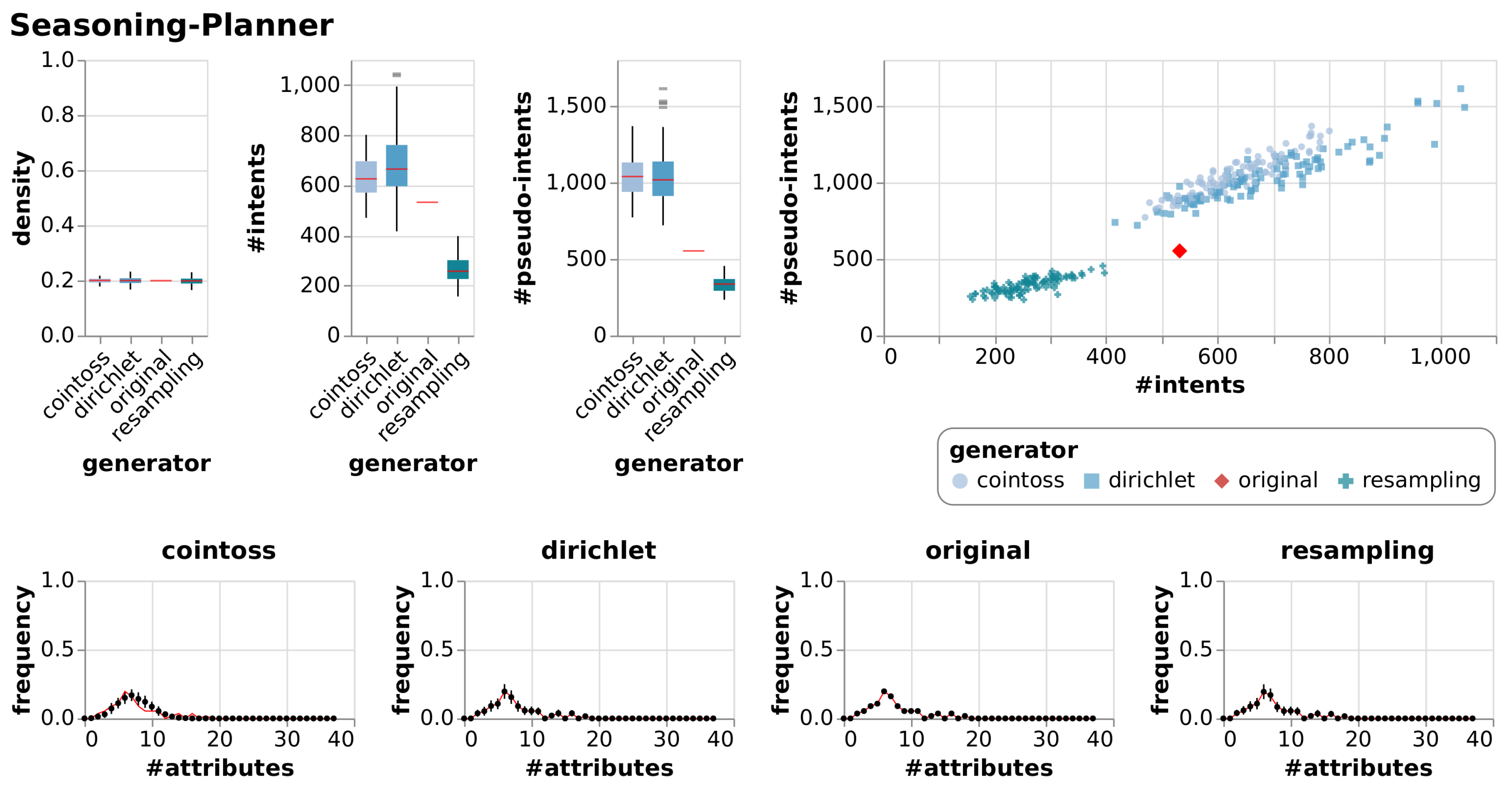
Figure A3.
Results of generating null models consisting of 100 random contexts each using resampling, coin-tossing and the Dirichlet approach, c.f. Figure 7.
Figure A3.
Results of generating null models consisting of 100 random contexts each using resampling, coin-tossing and the Dirichlet approach, c.f. Figure 7.

Figure A4.
Results of generating null models consisting of 100 random contexts each using resampling, coin-tossing and the Dirichlet approach, c.f. Figure 7.
Figure A4.
Results of generating null models consisting of 100 random contexts each using resampling, coin-tossing and the Dirichlet approach, c.f. Figure 7.
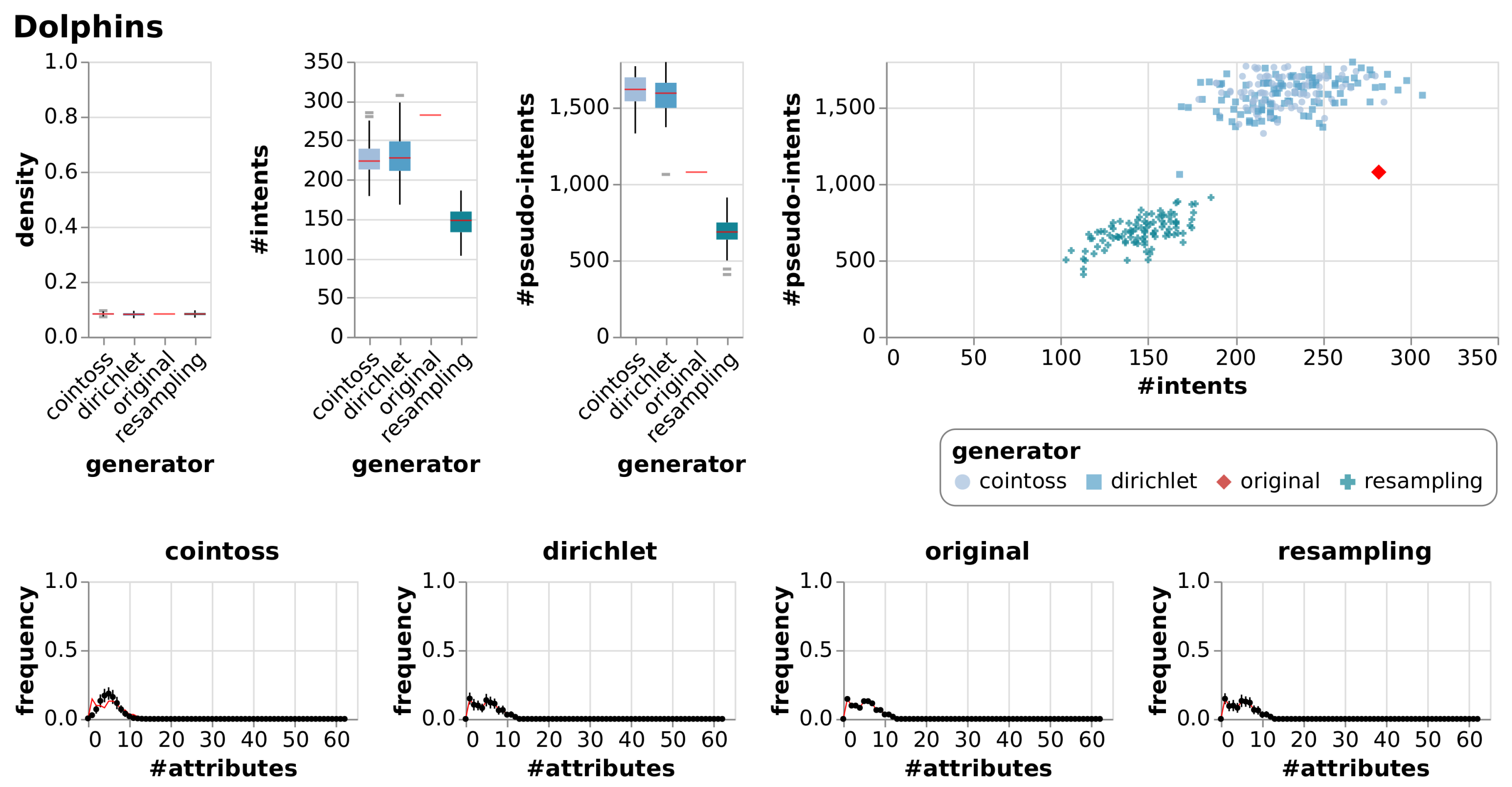
Figure A5.
Results of generating null models consisting of 100 random contexts each using resampling, coin-tossing and the Dirichlet approach, c.f. Figure 7.
Figure A5.
Results of generating null models consisting of 100 random contexts each using resampling, coin-tossing and the Dirichlet approach, c.f. Figure 7.

Figure A6.
Results of generating null models consisting of 100 random contexts each using resampling, coin-tossing and the Dirichlet approach, c.f. Figure 7.
Figure A6.
Results of generating null models consisting of 100 random contexts each using resampling, coin-tossing and the Dirichlet approach, c.f. Figure 7.
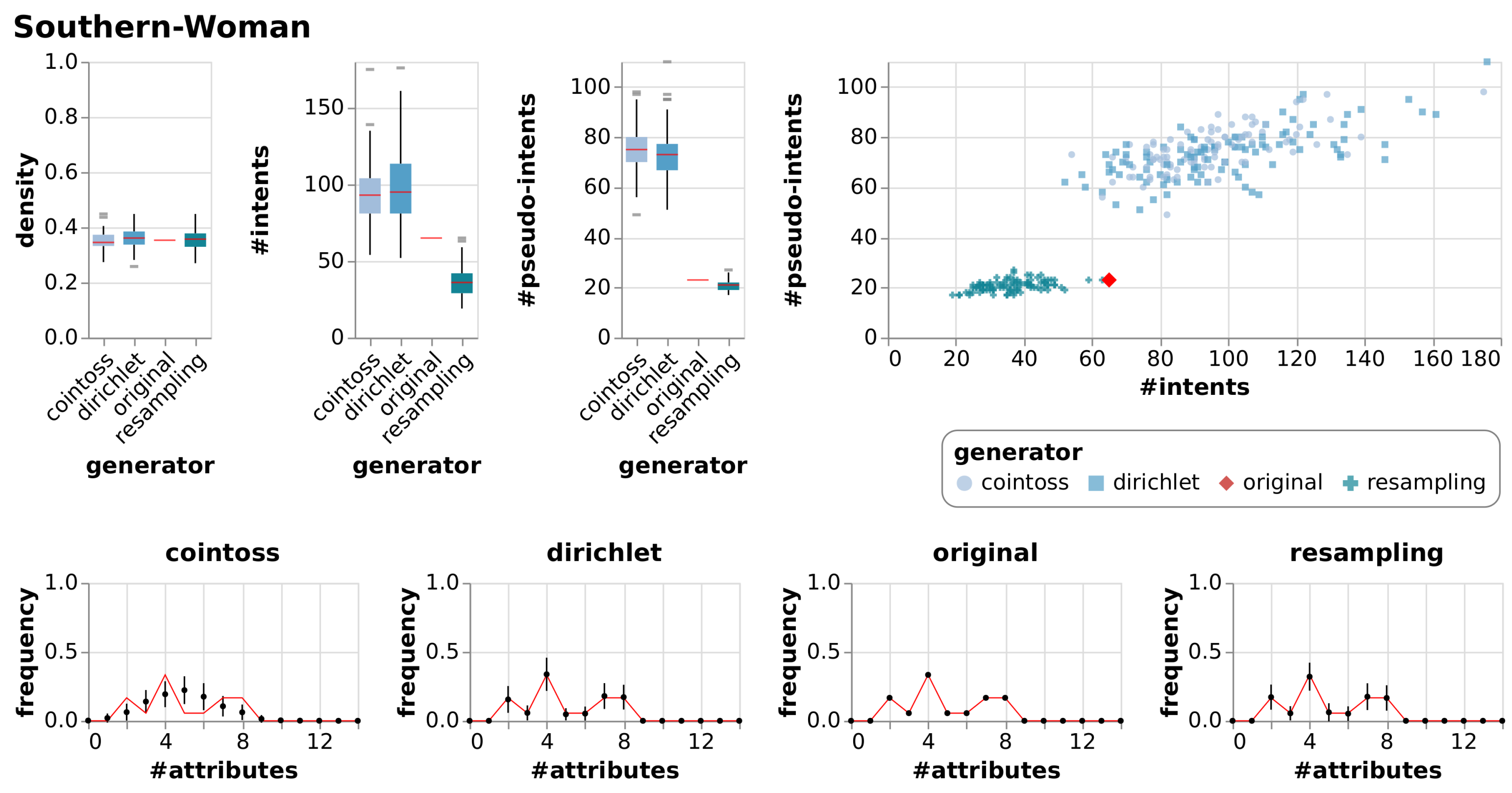
Figure A7.
Results of generating null models consisting of 100 random contexts each using resampling, coin-tossing and the Dirichlet approach, c.f. Figure 7.
Figure A7.
Results of generating null models consisting of 100 random contexts each using resampling, coin-tossing and the Dirichlet approach, c.f. Figure 7.

Figure A8.
Results of generating null models consisting of 100 random contexts each using resampling, coin-tossing and the Dirichlet approach, c.f. Figure 7.
Figure A8.
Results of generating null models consisting of 100 random contexts each using resampling, coin-tossing and the Dirichlet approach, c.f. Figure 7.

Figure A9.
Results of generating null models consisting of 100 random contexts each using resampling, coin-tossing and the Dirichlet approach, c.f. Figure 7.
Figure A9.
Results of generating null models consisting of 100 random contexts each using resampling, coin-tossing and the Dirichlet approach, c.f. Figure 7.
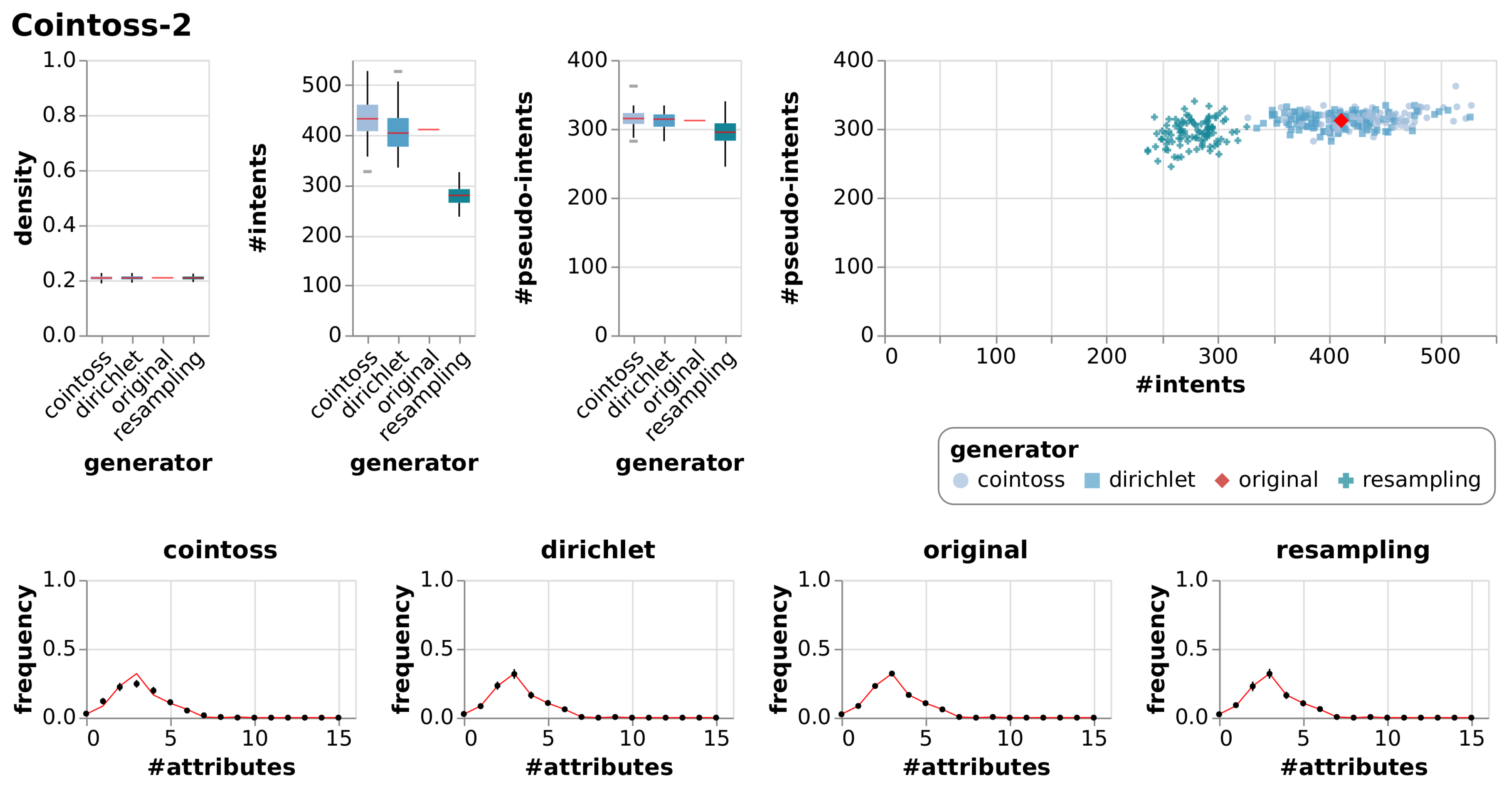
Figure A10.
Results of generating null models consisting of 100 random contexts each using resampling, coin-tossing and the Dirichlet approach, c.f. Figure 7.
Figure A10.
Results of generating null models consisting of 100 random contexts each using resampling, coin-tossing and the Dirichlet approach, c.f. Figure 7.
References
- Felde, M.; Hanika, T. Formal Context Generation Using Dirichlet Distributions. In Graph-Based Representation and Reasoning; Endres, D., Alam, M., Şotropa, D., Eds.; Springer International Publishing: Cham, Switzerland, 2019; pp. 57–71. [Google Scholar]
- Ganter, B.; Wille, R. Formal Concept Analysis: Mathematical Foundations; Springer: Berlin, Germany, 1999; pp. x+284. [Google Scholar]
- Newman, M.E.J. Finding community structure in networks using the eigenvectors of matrices. Phys. Rev. E 2006, 74, 036104. [Google Scholar] [CrossRef] [PubMed] [Green Version]
- Ulrich, W.; Gotelli, N.J. Pattern detection in null model analysis. Oikos 2013, 122, 2–18. [Google Scholar] [CrossRef] [Green Version]
- Gotelli, N.J. Null Model Analysis of Species Co-occurrence Patterns. Ecology 2000, 81, 2606–2621. [Google Scholar] [CrossRef]
- Kuznetsov, S.O.; Obiedkov, S.A. Comparing performance of algorithms for generating concept lattices. J. Exp. Theor. Artif. Intell. 2002, 14, 189–216. [Google Scholar] [CrossRef]
- Bazhanov, K.; Obiedkov, S.A. Comparing Performance of Algorithms for Generating the Duquenne-Guigues Basis. In Proceedings of the Eighth International Conference on Concept Lattices and Their Applications, Nancy, France, 17–20 October 2011; Napoli, A., Vychodil, V., Eds.; CEUR-WS.org: Aachen, Germany, 2011; Volume 959, pp. 43–57. [Google Scholar]
- Borchmann, D.; Hanika, T. Some Experimental Results on Randomly Generating Formal Contexts. In Proceedings of the Thirteenth International Conference on Concept Lattices and Their Applications, Moscow, Russia, 18–22 July 2016; Huchard, M., Kuznetsov, S.O., Eds.; CEUR-WS.org: Aachen, Germany, 2016; Volume 1624, pp. 57–69. [Google Scholar]
- Ganter, B. Random Extents and Random Closure Systems. In CLA; Napoli, A., Vychodil, V., Eds.; CEUR-WS.org: Aachen, Germany, 2011; Volume 959, pp. 309–318. [Google Scholar]
- Colomb, P.; Irlande, A.; Raynaud, O. Counting of Moore Families for n=7. In Formal Concept Analysis; Kwuida, L., Sertkaya, B., Eds.; Springer: Berlin/Heidelberg, Germany, 2010; pp. 72–87. [Google Scholar]
- Borchmann, D. Decomposing Finite Closure Operators by Attribute Exploration. In Contributions to ICFCA 2011; Domenach, F., Jäschke, R., Valtchev, P., Eds.; Univ. of Nicosia: Nicosia, Cyprus, 2011; pp. 24–37. [Google Scholar]
- Rimsa, A.; Song, M.A.J.; Zárate, L.E. SCGaz—A Synthetic Formal Context Generator with Density Control for Test and Evaluation of FCA Algorithms. In Proceedings of the IEEE International Conference on Systems, Man, and Cybernetics, Manchester, SMC 2013, Manchester, UK, 13–16 October 2013; pp. 3464–3470. [Google Scholar] [CrossRef]
- Ferguson, T.S. A Bayesian Analysis of Some Nonparametric Problems. Ann. Stat. 1973, 1, 209–230. [Google Scholar] [CrossRef]
- Hanika, T.; Hirth, J. Conexp-Clj—A Research Tool for FCA. In Proceedings of the Supplementary Proceedings of ICFCA 2019 Conference and Workshops, Frankfurt, Germany, 25–28 June 2019; CEUR-WS.org: Aachen, Germany, 2019; Volume 2378, pp. 70–75. [Google Scholar]
- Dawkins, B. Siobhan’s Problem: The Coupon Collector Revisited. Am. Stat. 1991, 45, 76–82. [Google Scholar]
- Onnela, J.P.; Arbesman, S.; González, M.C.; Barabási, A.L.; Christakis, N.A. Geographic constraints on social network groups. PLoS ONE 2011, 6, e16939. [Google Scholar] [CrossRef] [PubMed] [Green Version]
- Karsai, M.; Kivelä, M.; Pan, R.K.; Kaski, K.; Kertész, J.; Barabási, A.L.; Saramäki, J. Small but slow world: How network topology and burstiness slow down spreading. Phys. Rev. E 2011, 83, 025102. [Google Scholar] [CrossRef] [PubMed] [Green Version]
- Newman, M.E.J.; Girvan, M. Finding and evaluating community structure in networks. Phys. Rev. E 2004, 69, 026113. [Google Scholar] [CrossRef] [PubMed] [Green Version]
- Chung, F.; Lu, L. Connected Components in Random Graphs with Given Expected Degree Sequences. Ann. Comb. 2002, 6, 125–145. [Google Scholar] [CrossRef]
- Kunegis, J. KONECT: The Koblenz network collection. In Proceedings of the 22nd International World Wide Web Conference, WWW ’13, Rio de Janeiro, Brazil, 13–17 May 2013; Companion Volume; Carr, L., Laender, A.H.F., Lóscio, B.F., King, I., Fontoura, M., Vrandecic, D., Aroyo, L., De Oliveira, J.P.M., Lima, F., Wilde, E., Eds.; International World Wide Web Conferences Steering Committee/ACM: New York, NY, USA, 2013; pp. 1343–1350. [Google Scholar] [CrossRef]
- Faust, K. Centrality in Affiliation Networks. Soc. Netw. 1997, 19, 157–191. [Google Scholar] [CrossRef]
- Czerniak, J.; Zarzycki, H. Application of rough sets in the presumptive diagnosis of urinary system diseases. In Artificial Intelligence and Security in Computing Systems; Sołdek, J., Drobiazgiewicz, L., Eds.; Springer US: Boston, MA, USA, 2003; pp. 41–51. [Google Scholar]
- Dua, D.; Graff, C. UCI Machine Learning Repository; University of California: Irvine, CA, USA, 2017. [Google Scholar]
- Lusseau, D.; Schneider, K.; Boisseau, O.J.; Haase, P.; Slooten, E.; Dawson, S.M. The Bottlenose Dolphin Community of Doubtful Sound Features a Large Proportion of Long-Lasting Associations. Behav. Ecol. Sociobiol. 2003, 54, 396–405. [Google Scholar] [CrossRef]
- Felde, M.; Stumme, G. Interactive Collaborative Exploration using Incomplete Contexts. arXiv 2019, arXiv:1908.08740. [Google Scholar]
- Davis, A.; Gardner, B.B.; Gardner, M.R. Deep South; a Social Anthropological Study of Caste and Class; The University of Chicago Press: Chicago, IL, USA, 1941. [Google Scholar]
- Watts, D.J.; Strogatz, S.H. Collective dynamics of ‘small-world’ networks. Nature 1998, 393, 440–442. [Google Scholar] [CrossRef] [PubMed]
Figure 1.
Visualization of I-PI-coordinates for coin-tossing, see Example 1.
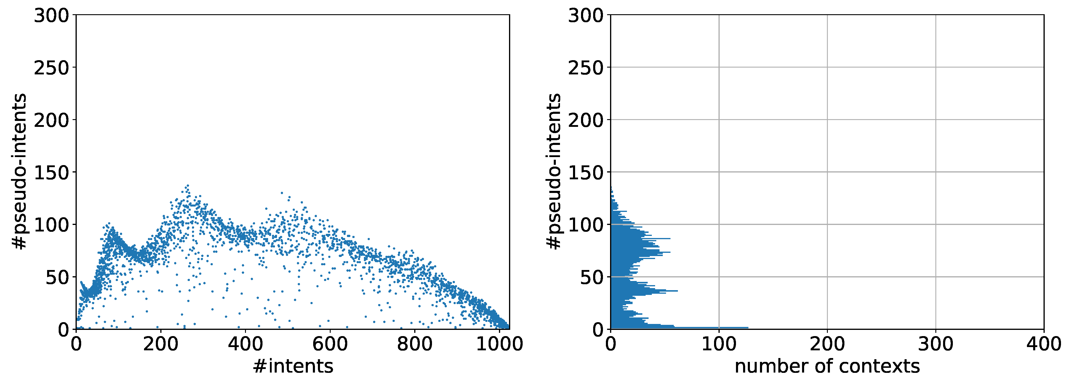
Figure 2.
Distribution of categorical probabilities of sym. Dirichlet distributions.

Figure 3.
Dirichlet generated contexts with , .
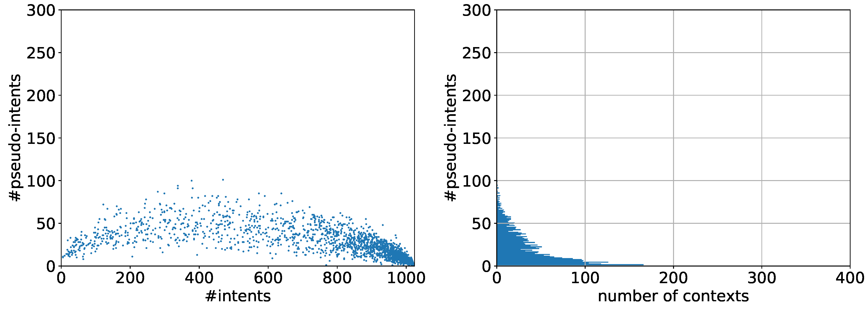
Figure 4.
Dirichlet generated contexts with , .
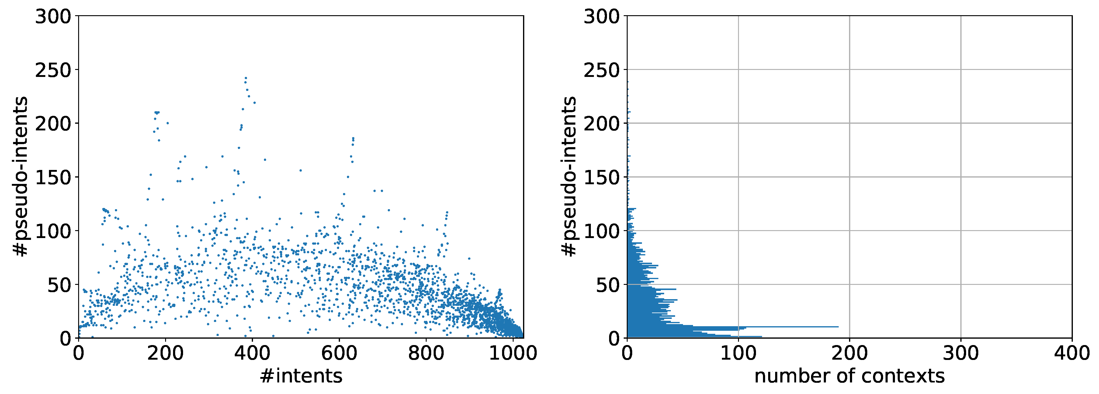
Figure 5.
Dirichlet generated contexts with , .
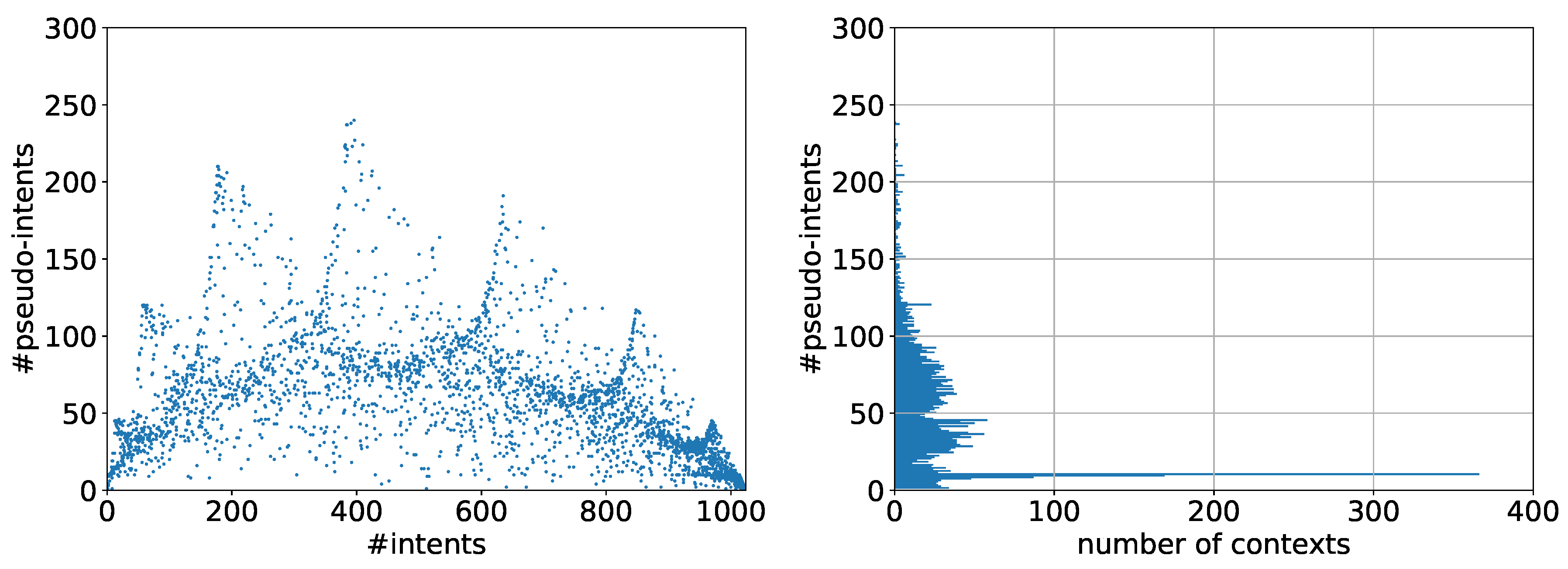
Figure 6.
Number of distinct I-PI coordinates for up to 100,000 randomly generated contexts with 6, 7 and 8 attributes.
Figure 6.
Number of distinct I-PI coordinates for up to 100,000 randomly generated contexts with 6, 7 and 8 attributes.
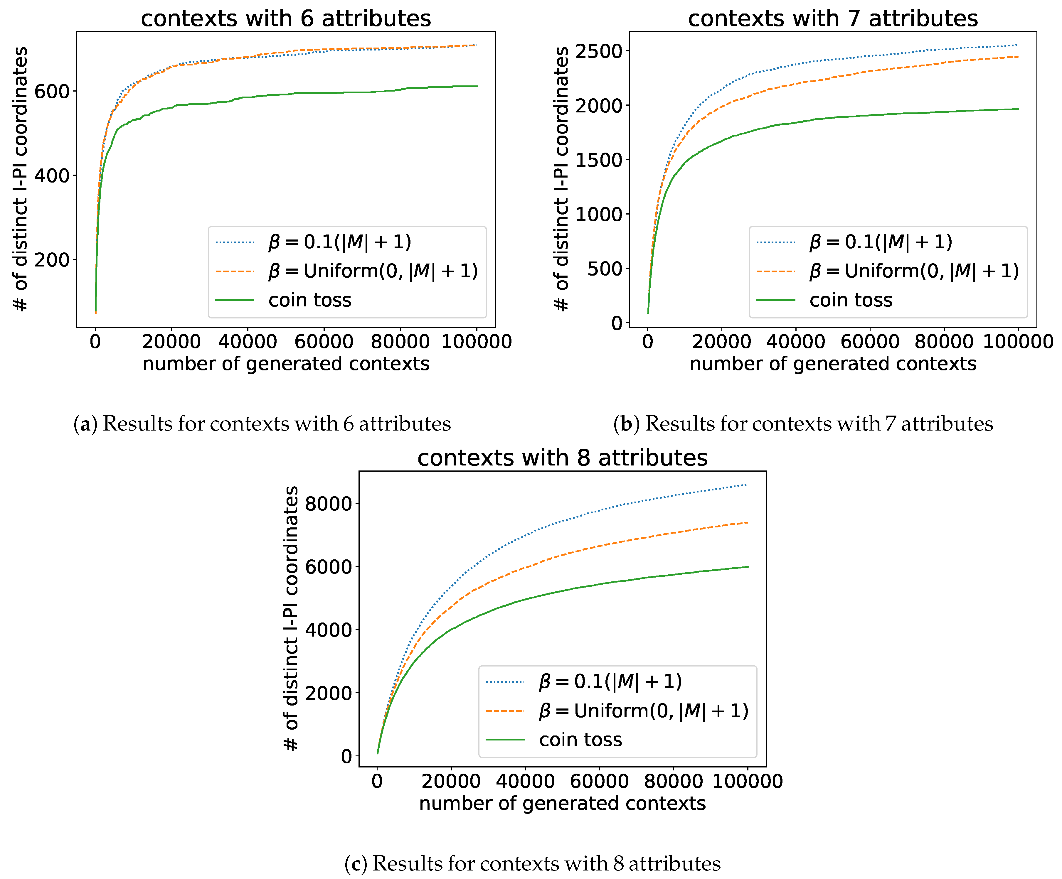
Figure 7.
Results of generating null models consisting of 100 random contexts each using resampling, coin-tossing and the Dirichlet approach. The first three charts show the resulting densities, numbers of intents and numbers of pseudo-intents as box-whiskers plots with outliers. The chart in the top right is an I-PI-plot of all generated contexts. The four other charts depict the mean and standard deviation of the frequencies of the numbers of attributes, i.e., of the row sum distributions. The red line indicates the row sum distribution of the original context for which the null models were generated.
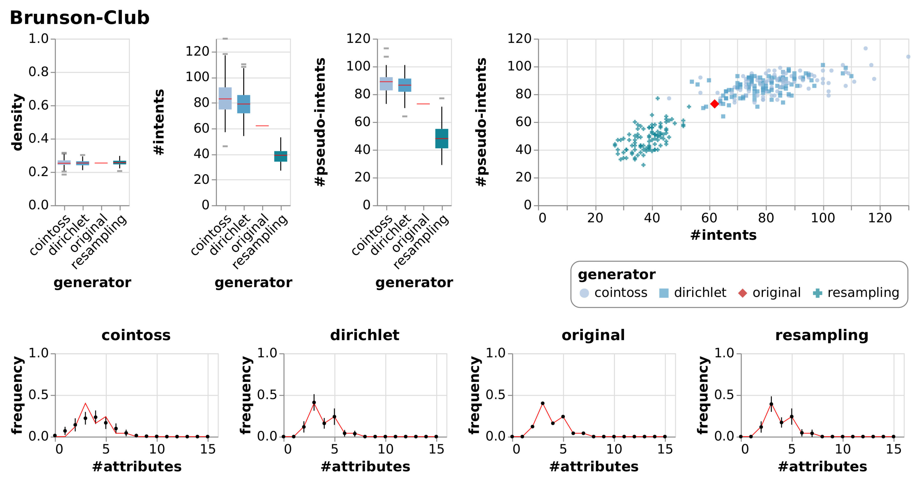
Figure 8.
Results of generating null models consisting of 100 random contexts each using resampling, coin-tossing and the Dirichlet approach, c.f. Figure 7.
Figure 8.
Results of generating null models consisting of 100 random contexts each using resampling, coin-tossing and the Dirichlet approach, c.f. Figure 7.

Figure 9.
Results of generating null models consisting of 100 random contexts each using resampling, coin-tossing and the Dirichlet approach, c.f. Figure 7.
Figure 9.
Results of generating null models consisting of 100 random contexts each using resampling, coin-tossing and the Dirichlet approach, c.f. Figure 7.
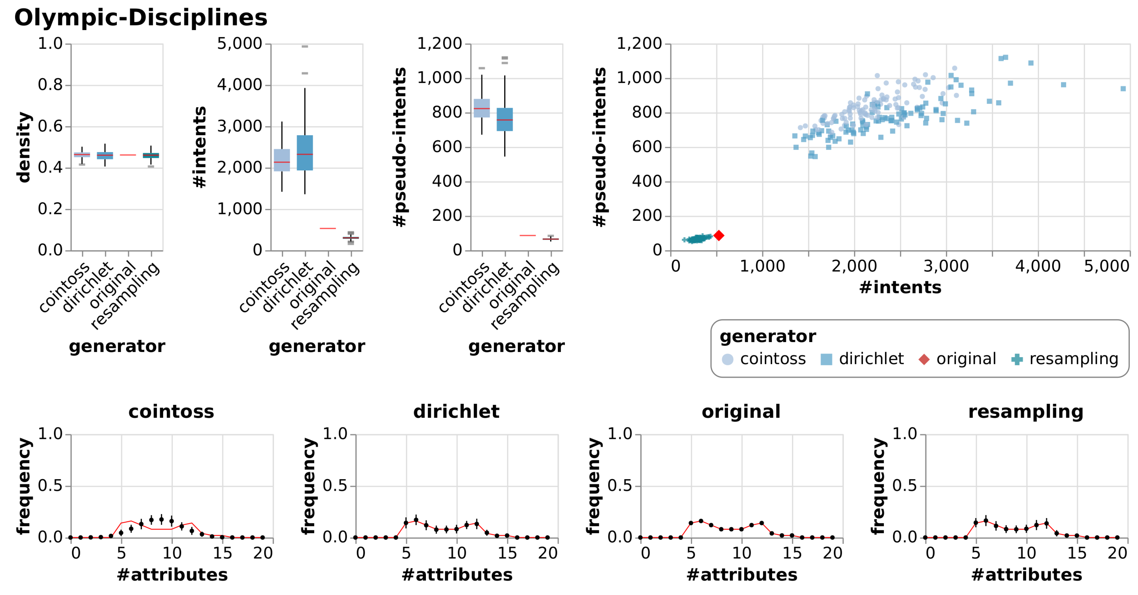
Figure 10.
Results of generating null models consisting of 100 random contexts each using resampling, coin-tossing and the Dirichlet approach, c.f. Figure 7.
Figure 10.
Results of generating null models consisting of 100 random contexts each using resampling, coin-tossing and the Dirichlet approach, c.f. Figure 7.


Table 1.
Non-exhaustive list of methods for simple null models under the indicated constraints. We write G-dist for the row sum distribution and M-dist for the column sum distribution of a formal context. Further we write (G-dist) and (M-dist) for the expected row (column) sum distribution.
Table 1.
Non-exhaustive list of methods for simple null models under the indicated constraints. We write G-dist for the row sum distribution and M-dist for the column sum distribution of a formal context. Further we write (G-dist) and (M-dist) for the expected row (column) sum distribution.
| Constraint | Randomization Method(s) for Null Models |
|---|---|
| keep G-dist and M-dist | pairwise swapping of incidences |
| keep G-dist or M-dist | shuffling of rows or columns |
| keep (G-dist) or (M-dist) | Dirichlet approach based on the row sum distribution as base measure and a high precision parameter. |
| keep (density) | coin-toss based on density, Dirichlet approach |
| keep all implications | resampling of objects |
Table 2.
Dataset Descriptions. All considered contexts can be found online contained in the conexp-clj software, see [14], or in the supplementary materials for this paper, see Section 5 on page 7.
| Context | Source | Description |
|---|---|---|
| Bird-Diet | [14] | A context of birds and what they eat. |
| Brunson-Club | [20,21] | Membership information of corporate executive officers in social organisations. |
| Diagnosis | [22,23] | The data was created by a medical expert as a data set to test the expert system, which will perform the presumptive diagnosis of two diseases of the urinary system. The temperature attribute is interval-scaled. |
| Dolphins | [20,24] | A formal context created from a directed social network of bottlenose dolphins living in a fjord in New Zealand. A relation indicates frequent association based on observations between 1994 and 2001. |
| Forum-Romanum | [2] | A context based on ratings of monuments on the Forum Romanum in different travel guides and scaled ordinally. This context can be found in the standard work on FCA. |
| Living-Beings-and-Water | [2] | The first formal context in the standard work on FCA (the yellow book) by Ganter and Wille. |
| Olympic-Disciplines | [25] | This context is about the disciplines of the Summer Olympic Games 2020. |
| Seasoning-Planner | [14] | This context contains foods that are related to recommended seasonings based on a chart published by the spice company Fuchs Group. |
| Southern-Woman | [20,26] | Participation of 18 white women in 14 social events over a nine-month period, collected in the Southern United States of America in the 1930s. |
| Wood-Properties | [14] | A context about properties of different kinds of wood. |
| Cointoss-1 | artificial | Artificially generated with the coin-toss approach. |
| Cointoss-2 | artificial | Artificially generated with the coin-toss approach. |
| Dirichlet-1 | artificial | Artificially generated with the Dirichlet approach. |
| Dirichlet-2 | artificial | Artificially generated with the Dirichlet approach. |
Table 3.
This table contains some basic properties of the formal contexts used in the experiment where each method of random generation was used to generate a null model consisting of 100 contexts. The aggregated results for density, number of intents and number of pseudo-intents are shown.
Table 3.
This table contains some basic properties of the formal contexts used in the experiment where each method of random generation was used to generate a null model consisting of 100 contexts. The aggregated results for density, number of intents and number of pseudo-intents are shown.
| Context | Method | #Attributes | #Objects | ()-Density | -Density | ()-#Intents | -#Intents | ()-#Pseudo-Intents | -#Pseudo-Intents |
|---|---|---|---|---|---|---|---|---|---|
| Bird-Diet | True Context | 8 | 10 | 0.30 | 16 | 15 | |||
| Cointoss | 0.30 | 0.05 | 18 | 3.87 | 15 | 2.85 | |||
| Dirichlet | 0.30 | 0.04 | 18 | 3.50 | 15 | 2.49 | |||
| Resample | 0.30 | 0.05 | 11 | 2.01 | 11 | 1.81 | |||
| Brunson-Club | True Context | 15 | 25 | 0.25 | 62 | 73 | |||
| Cointoss | 0.25 | 0.02 | 84 | 14.18 | 88 | 7.41 | |||
| Dirichlet | 0.25 | 0.02 | 79 | 10.86 | 86 | 7.17 | |||
| Resample | 0.26 | 0.02 | 39 | 5.73 | 48 | 8.94 | |||
| Diagnosis | True Context | 17 | 120 | 0.47 | 88 | 43 | |||
| Cointoss | 0.47 | 0.01 | 5749 | 779.98 | 1422 | 100.19 | |||
| Dirichlet | 0.47 | 0.00 | 3677 | 55.04 | 1420 | 38.12 | |||
| Resample | 0.47 | 0.00 | 87 | 1.94 | 43 | 0.74 | |||
| Dolphins | True Context | 62 | 62 | 0.08 | 282 | 1077 | |||
| Cointoss | 0.08 | 0.00 | 227 | 21.15 | 1611 | 97.30 | |||
| Dirichlet | 0.08 | 0.01 | 231 | 29.73 | 1580 | 117.76 | |||
| Resample | 0.08 | 0.01 | 146 | 18.26 | 685 | 97.01 | |||
| Forum-Romanum | True Context | 7 | 14 | 0.45 | 19 | 8 | |||
| Cointoss | 0.45 | 0.05 | 33 | 7.29 | 13 | 1.92 | |||
| Dirichlet | 0.45 | 0.08 | 27 | 10.84 | 12 | 2.79 | |||
| Resample | 0.46 | 0.09 | 13 | 2.48 | 8 | 1.10 | |||
| Living-Beings-and-Water | True Context | 9 | 8 | 0.47 | 19 | 10 | |||
| Cointoss | 0.46 | 0.06 | 28 | 6.71 | 18 | 3.23 | |||
| Dirichlet | 0.47 | 0.02 | 29 | 4.34 | 19 | 3.57 | |||
| Resample | 0.47 | 0.03 | 12 | 2.47 | 10 | 0.78 | |||
| Olympic-Disciplines | True Context | 19 | 50 | 0.46 | 529 | 86 | |||
| Cointoss | 0.46 | 0.02 | 2178 | 380.38 | 831 | 83.09 | |||
| Dirichlet | 0.46 | 0.02 | 2414 | 674.88 | 773 | 114.78 | |||
| Resample | 0.46 | 0.02 | 301 | 47.00 | 65 | 6.51 | |||
| Seasoning-Planner | True Context | 37 | 56 | 0.20 | 532 | 553 | |||
| Cointoss | 0.20 | 0.01 | 631 | 83.08 | 1045 | 133.45 | |||
| Dirichlet | 0.20 | 0.01 | 688 | 131.33 | 1044 | 172.95 | |||
| Resample | 0.20 | 0.01 | 260 | 52.03 | 331 | 49.12 | |||
| Southern-Woman | True Context | 14 | 18 | 0.35 | 65 | 23 | |||
| Cointoss | 0.35 | 0.03 | 94 | 18.59 | 75 | 8.57 | |||
| Dirichlet | 0.36 | 0.04 | 99 | 25.07 | 73 | 10.09 | |||
| Resample | 0.35 | 0.04 | 36 | 9.00 | 21 | 2.15 | |||
| Wood-Properties | True Context | 28 | 29 | 0.28 | 315 | 275 | |||
| Cointoss | 0.28 | 0.01 | 362 | 54.30 | 432 | 42.88 | |||
| Dirichlet | 0.28 | 0.02 | 361 | 61.43 | 427 | 45.90 | |||
| Resample | 0.29 | 0.02 | 154 | 31.96 | 153 | 31.68 | |||
| Cointoss-1 | True Context | 10 | 793 | 0.42 | 913 | 34 | |||
| Cointoss | 0.42 | 0.01 | 866 | 27.40 | 45 | 8.39 | |||
| Dirichlet | 0.42 | 0.01 | 880 | 29.42 | 42 | 8.97 | |||
| Resample | 0.42 | 0.01 | 808 | 28.68 | 49 | 6.40 | |||
| Cointoss-2 | True Context | 15 | 200 | 0.21 | 411 | 312 | |||
| Cointoss | 0.21 | 0.01 | 434 | 39.18 | 315 | 12.16 | |||
| Dirichlet | 0.21 | 0.01 | 408 | 40.04 | 312 | 11.37 | |||
| Resample | 0.21 | 0.01 | 278 | 19.39 | 294 | 18.59 | |||
| Dirichlet-1 | True Context | 10 | 198 | 0.39 | 308 | 101 | |||
| Cointoss | 0.39 | 0.01 | 467 | 42.57 | 80 | 6.24 | |||
| Dirichlet | 0.39 | 0.01 | 307 | 7.04 | 96 | 4.40 | |||
| Resample | 0.39 | 0.01 | 259 | 7.21 | 84 | 6.61 | |||
| Dirichlet-2 | True Context | 15 | 200 | 0.57 | 18,166 | 564 | |||
| Cointoss | 0.57 | 0.01 | 12,451 | 1053.37 | 989 | 80.60 | |||
| Dirichlet | 0.57 | 0.01 | 17,894 | 1342.92 | 625 | 68.66 | |||
| Resample | 0.57 | 0.01 | 12,018 | 976.22 | 552 | 51.81 |
© 2020 by the authors. Licensee MDPI, Basel, Switzerland. This article is an open access article distributed under the terms and conditions of the Creative Commons Attribution (CC BY) license (http://creativecommons.org/licenses/by/4.0/).
Share and Cite
MDPI and ACS Style
Felde, M.; Hanika, T.; Stumme, G. Null Models for Formal Contexts. Information 2020, 11, 135. https://doi.org/10.3390/info11030135
AMA Style
Felde M, Hanika T, Stumme G. Null Models for Formal Contexts. Information. 2020; 11(3):135. https://doi.org/10.3390/info11030135
Chicago/Turabian StyleFelde, Maximilian, Tom Hanika, and Gerd Stumme. 2020. "Null Models for Formal Contexts" Information 11, no. 3: 135. https://doi.org/10.3390/info11030135
Note that from the first issue of 2016, this journal uses article numbers instead of page numbers. See further details here.