Spectral Normalization for Domain Adaptation

Abstract

The transfer learning method is used to extend our existing model to more difficult scenarios, thereby accelerating the training process and improving learning performance. The conditional adversarial domain adaptation method proposed in 2018 is a particular type of transfer learning. It uses the domain discriminator to identify which images the extracted features belong to. The features are obtained from the feature extraction network. The stability of the domain discriminator directly affects the classification accuracy. Here, we propose a new algorithm to improve the predictive accuracy. First, we introduce the Lipschitz constraint condition into domain adaptation. If the constraint condition can be satisfied, the method will be stable. Second, we analyze how to make the gradient satisfy the condition, thereby deducing the modified gradient via the spectrum regularization method. The modified gradient is then used to update the parameter matrix. The proposed method is compared to the ResNet-50, deep adaptation network, domain adversarial neural network, joint adaptation network, and conditional domain adversarial network methods using the datasets that are found in Office-31, ImageCLEF-DA, and Office-Home. The simulations demonstrate that the proposed method has a better performance than other methods with respect to accuracy.

1. Introduction

Deep learning is a subset of machine learning, which is a subfield of artificial intelligence. Deep learning has been widely applied, for example, in natural language processing, medical imaging analysis, remote-sensing image analysis, and synthetic aperture radar (SAR) target recognition [1,2,3,4,5]. If the training dataset is insufficient, this insufficiency will affect the recognition accuracy. In some applications, it is difficult to collect enough training data. Furthermore, manual annotation labels are also considerably time-consuming [6]. In order to solve these problems, the transfer learning method is used in deep learning. This method can search annotated data that are similar, transferring learning to the target data and thereby increasing the size of the target dataset and improving the performance of deep learning. Transfer learning can be used to transfer labels or data structures from the Source domain (training dataset of other objects) to the Target domain (training dataset of the current object) in order to improve the learning effect [7].

Transfer learning can be divided into two categories: heterogeneous transfer learning and homogeneous transfer learning. In heterogeneous transfer learning, the Source and Target datasets are different in both their features and label spaces. In homogeneous transfer learning, the Source and Target datasets are the same in both their features and label spaces. Domain adaptation is one form of homogeneous transfer learning. It is used to search the shared features between the Source and Target domains in a high dimensional space [8]. Domain adaptation can be divided into the distribution adaptation, subspace learning, and feature representation transfer methods. The distribution adaptation method is a commonly used method of domain adaptation. This method can reduce the distribution distance between the Source and Target domains by applying certain transformations [9,10]. The subspace learning method assumes that the subspace distribution of the Source domain and the Target domain remains the same after transformation [11,12]. The feature representation transfer method searches for similar features between the Source and Target domains to realize domain adaptation. There are several methods involved in feature representation transfer, such as the feature selection and structure preservation (FSSL) method [13]. This method uses feature selection to find the same information for both the Source domain and Target domain to solve the issue of domain adaptation.

The deep adaptation networks (DAN) method [14] uses three adaptation layers that lie behind the feature extraction layer to calculate the distance between the Source and Target domains. The adaptation layer is a layer in the networks that is used to examine the whole network’s ability to distinguish the Source domain and Target domain. The smaller the distance measurement is, the better the network’s performance is. Based on the DAN method, the joint adaptation network (JAN) method [15] proposed a joint distribution measurement (JMMD) method which not only puts the data into the adaptation layer, but also includes the labels of the data together in the adaptation layer. The residual transfer network (RTN) [16] method does not involve the assumption that the Source and Target domains share one classifier; instead, it uses two domain classifiers and a residual function to calculate the difference between the Source classifier and Target classifiers. This can reduce the domain differences. The joint convolutional neural network architecture for the domain and task transfer method [17] proposes simultaneous transfer of the domain and task. It uses the class distribution relationship of the Source domain to constrain the Target domain. The adaptive batch normalization (AdaBN) method [18] does not involve an additional adaptive layer in the network but instead adds the adaptation of statistical features into the normalization layer in order to complete the transfer. It does not require additional components and parameters, making it very simple and effective.

Ganin Yaroslav was the first person to add the generative adversarial network to the domain adaptation network to measure the data distribution difference between the Source and Target domains [19]. The generative adversarial network [20] is used to generate data to extend an existing dataset, but the generated data and real data cannot be distinguished by the discriminator. Based on the proposed framework, the adversarial discriminative domain adaptation (ADDA) method [21] proposes a generic framework of domain adaptation that uses the adversarial network. This method uses the generative adversarial network loss function as the loss function of the proposed network, and adds the discriminative network to the proposed network. The ADDA method can complete transfer learning when the data distribution of the Source domain and Target domain features a large difference. The conditional adversarial domain adaptation (CDAN) method [22] uses a multilinear map to combine the features and labels from the Source domain and Target domains, adding the information entropy into the loss function to reduce the adverse effect of the samples that are difficult to transfer. The information entropy is $H\left(g\right)=-{\displaystyle \sum _{c=1}^C{g}_c\log g_c}$ ($C$ is the total number of classes and $g_c$ is the probability of predicting an example for class $c$). There are further domain adaptation methods that can be used when searching for domain invariant features in which the features are shared by the Source and Target domains. The Wasserstein distance guided representation learning (WDGRL) method [23] uses the Wasserstein distance [24] to calculate the difference in the distance between the Source and Target domains. The cycle-consistent adversarial domain adaptation (CyCADA) method [25] constructs a network to search for optimal shared features between the Source and Target domains. This network is used to generate a Target domain from the Source domain, and to generate a Source domain from the generated Target domain. The whole domain generation process is cyclic, so it is called a circular network. In unsupervised image-to-image translation (UNIT) [26], a network framework is designed that is used to learn the joint distribution of different domains by using marginal distribution. The selective adversarial networks (SAN) method [27] proposes partial transfer learning to solve the problem of a Source domain that has far more data categories than the Target domain.

In Section 1, we introduced transfer learning and some related algorithms concerning domain adaptation. The conditional adversarial domain adaptation (CDAN) method is introduced in detail in Section 2. The proposed method is then presented in Section 3. In Section 4, the simulation is presented and discussed.

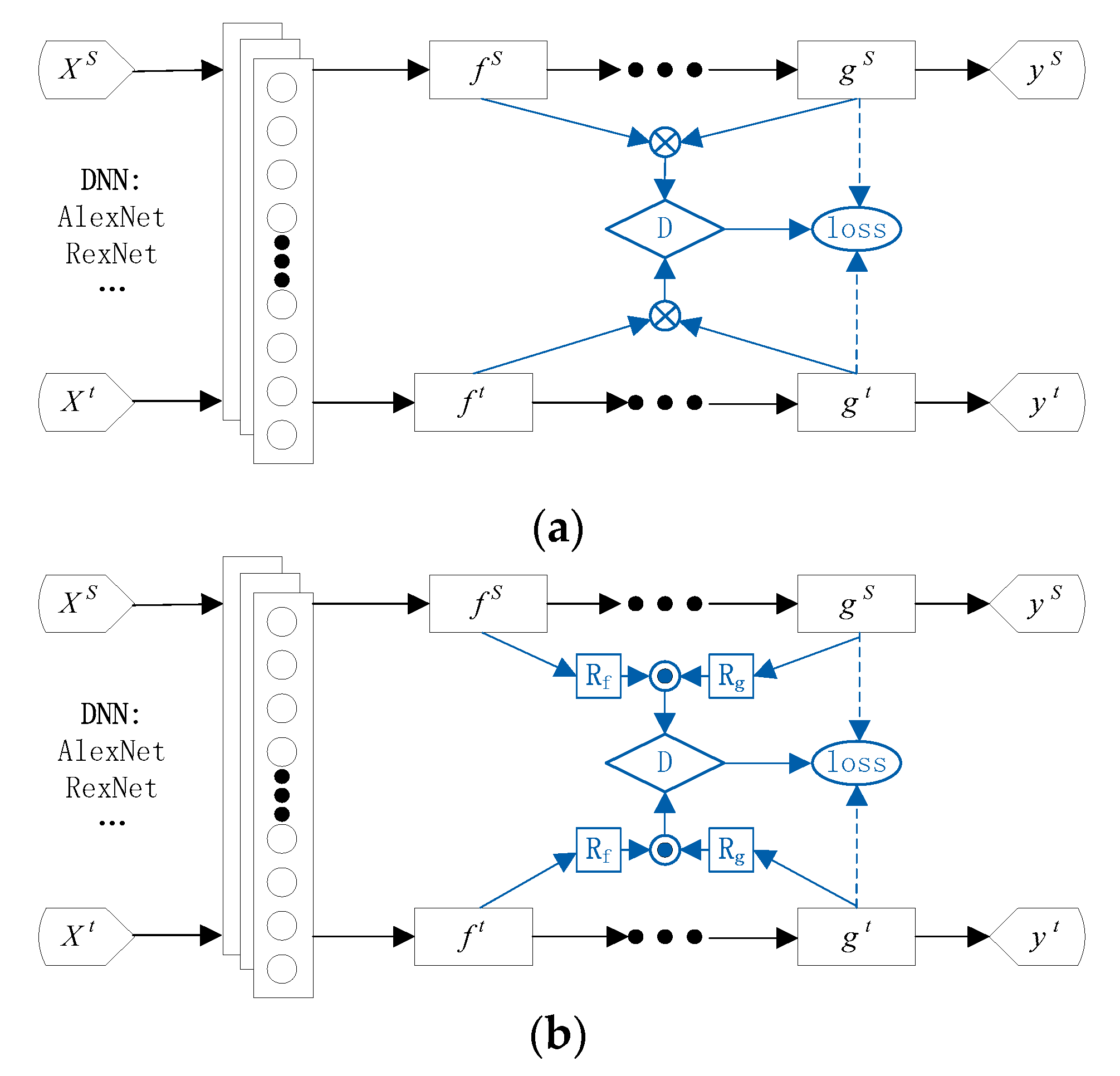
2. Conditional Adversarial Domain Adaptation

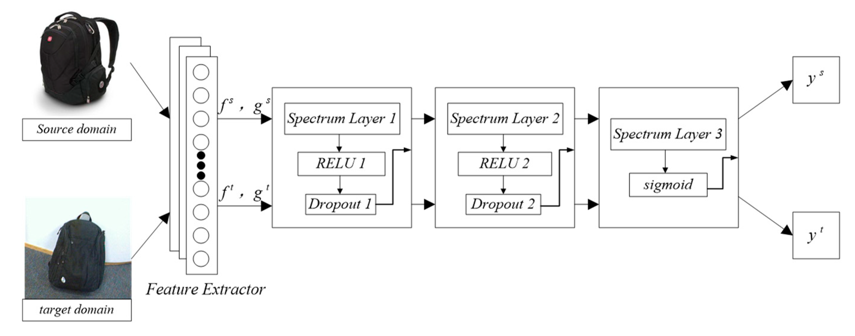
Although domain adaptation can help to solve a dataset that lacks labels, for domain adaptation, which uses an adversarial network, some problems remain. First, the previous algorithms only aligned the features of the data without also considering the labels. Second, if the modal structure of the data features is highly complex, the current domain adaptation method—which uses an adversarial network—cannot locate the multimodal structures, representing a simple cause of negative transfer. Third, the minimax optimization method in the conditional domain discriminator imposes different examples that have equal importance. This may result in adverse effects of hard-to-transfer examples upon domain adaptation.

In order to solve these problems, a conditional adversarial domain adaptation (CDAN) method is proposed [22]. The framework of the CDAN is outlined in Figure 1. In adversarial domain adaptation, the classifier prediction result carries potentially discriminant information revealing multimodal results. This potentially discriminant information is used to align the appropriate features to capture multimodal information during network training. Based on this, the CDAN method combines features and labels that are introduced to domain adaptation to obtain the loss function, which can be expressed as:

$$\underset{G}{\min }\epsilon \left(G\right)-\lambda \epsilon (D,G),$$

(1)

$$\underset{D}{\min }\epsilon (D,G),$$

(2)

where $\lambda$ is a hyper parameter between the two objectives for the tradeoff source risk and domain adversary; $\epsilon \left(G\right)$ is located on the source classifier $G$ and $\epsilon \left(D,G\right)$ on the source classifier $G$ and domain discriminator $D$, which are respectively expressed as:

$$\epsilon \left(G\right)=E_{(x_i^s,y_i^s)~D^s}L\left(G\left(x_i^s\right),y_i^s\right),$$

(3)

$$\epsilon (D,G)=-E_{x_i^s~D^s}\log [D(f_i^s,g_i^s)]-E_{x_j^t~D^t}\log [1-D(f_j^t,g_j^t)],$$

(4)

where $f$ and $g$ are the feature and label of the Source domain and Target domain, respectively, $L()$ is the cross-entropy loss function, $s$ is the Source domain and $t$ is the Target domain.

The CDAN method uses a multilinear map to connect $f$ and $g$ to form $h=\left(f,g\right)$—this can represent the relationship between features and labels. $f\otimes g$ represents a multilinear map, and $\otimes$ is tensor multiplication. However, when the dimensions of the feature and label are large, the dimension of $f\otimes g$ is $d_f\times d_g$ and will suffer from exploding gradient problems. The authors addressed this issue by randomly selecting some dimensions of $f$ and $g$ to construct a multilinear map:

$$T\odot \left(f,g\right)=\frac{1}{\sqrt{d}}\left(R_{f}f\right)\odot \left(R_{g}g\right),$$

(5)

where $\odot$ is the element-wise product, $R_f$ and $R_g$ are random matrices which are only sampled once and are fixed during training, and $d$ is the dimension. CDAN finds that $T_{\otimes }=T_{\odot }$ is in a high-dimensional space. Thus, when the dimensional multiplication of $f$ and $g$ is greater than 4096, a random strategy is used for the multilinear map. Otherwise, the normal multilinear map is used:

$$T\left(h\right)=\{\begin{array}{cc}{T}_{\otimes }\left(f,g\right)& d_f\times d_g\le 4096\\ T_{\odot }\left(f,g\right)& otherwise\end{array}.$$

(6)

Furthermore, the CDAN method uses entropy $H\left(g\right)=-{\displaystyle \sum _{c=1}^C{g}_c\log g_c}$($C$ is the total number of classes and $g_c$ is the probability of predicting for example to class $c$) to calculate the uncertainty of the predicted result of the classifier. The certainty of the predicted result is expressed as:

$$\omega \left(H\left(g\right)\right)=1+e^{-H\left(g\right)},$$

(7)

and then the loss function in (1) and (2) can be expressed as:

$$\begin{array}{l}\underset{G}{\min }{E}_{\left(x_i^s,y_i^s\right)~D_s}L\left(G\left(x_i^s\right),y_i^s\right)\\ +\lambda \left(E_{x_i^s~D^s}\omega \left(H\left(g_i^s\right)\right)\log \left[D\left(T\left(h_i^s\right)\right)\right]+E_{x_j^t~D^t}\omega \left(H\left(g_j^t\right)\right)\log \left[D\left(T\left(h_j^t\right)\right)\right]\right)\end{array}$$

(8)

$$\underset{D}{\max }{E}_{x_i^s~D^s}\omega \left(H\left(g_i^s\right)\right)\log \left[D\left(T\left(h_i^s\right)\right)\right]+E_{x_j^t~D^t}\omega \left(H\left(g_j^t\right)\right)\log \left[D\left(T\left(h_j^t\right)\right)\right].$$

(9)

Following the concepts introduced above, the network structure of CDAN is presented in Figure 1. Figure 1a illustrates the network structure in a low-dimensional scenario, while Figure 1b features the network structure in a high-dimensional scenario.

3. Proposed Method

The conditional domain adversarial network (CDAN) adds an adversarial network into domain adaptation in order to search for a domain invariant feature. This adversarial network is composed of a label classifier, feature extractor, and domain discriminator. The better the domain discriminator performs, the more significantly the feature extractor gradient disappears. When the domain discriminator is trained too well, the gradient of the feature extractor will reach zero, and when the domain discriminator is trained too poorly, the gradient of the feature extractor does not decrease. Only when the training of the domain discriminator is neither good nor bad does the feature extractor exhibit a better performance.

To overcome this problem, we introduced the 1-Lipschitz constraint condition into the adversarial network of the CDAN method. The Lipschitz constraint condition is:

$$\frac{{\Vert f\left(x+\delta \right)-f\left(x\right)\Vert }_2}{{\Vert \delta \Vert }_2}\le 1,$$

(10)

where $f()$ is a function, $x$ is a variable, and $\delta$ is a smaller variable. In the proposed method, the output of the $n$th layer can be expressed as:

$$X_n=f\left(W_n{X}_{n-1}+b_n\right),$$

(11)

where $X_n$ is output of the $n$th layer, $f()$ is an activation function that corresponds to the function $f()$ in (10), $X_{n-1}$ is output of $(n-1)$th layer, $W_n$ and $b_n$ are the parameter matrix and bias of the network in the $n$ layer, respectively. The activation function is a ReLU (Rectified Linear Unit) function, so the bias units can be ignored. Therefore, the output of the $n$th layer in (11) can be simplified as follows:

$$X_n=D_n{W}_n{X}_{n-1},$$

(12)

where $D_n$ is a diagonal matrix that is obtained by using the ReLU function as an activation function in (11). In this way, the relationship between the output of the $n$th layer and input can be expressed as:

$$X_n(X_0)=D_n{W}_n{D}_{n-1}{W}_{n-1}\cdots D_2{W}_2{D}_1{W}_1{X}_0,$$

(13)

and the norm of gradient $X_n$ can be expressed as:

$$\begin{array}{ll}{\Vert \nabla X_n\Vert }_2& =\frac{{\Vert X_n\left(X_0+\delta \right)-X_n\left(X_0\right)\Vert }_2}{{\Vert \delta \Vert }_2}\\ & =\frac{{\Vert D_n{W}_n{D}_{n-1}{W}_{n-1}\cdots D_2{W}_2{D}_1{W}_1\left(X_0+\delta \right)-D_n{W}_n{D}_{n-1}{W}_{n-1}\cdots D_2{W}_2{D}_1{W}_1{X}_0\Vert }_2}{{\Vert \delta \Vert }_2}\\ & =\frac{{\Vert D_n{W}_n{D}_{n-1}{W}_{n-1}\cdots D_2{W}_2{D}_1{W}_1\delta \Vert }_2}{{\Vert \delta \Vert }_2}\end{array}$$

(14)

where ${\Vert \nabla X_n\Vert }_2$ is the gradient of $X_n$, and $\delta$ is a smaller variable around $X_0$. According to the computation method of the maximum singular value of the matrix:

$$\underset{\Vert \delta \Vert \ne 0}{\max }\frac{{\Vert M\delta \Vert }_2}{{\Vert \delta \Vert }_2}=\underset{\Vert \delta \Vert =1}{\max }{\Vert M\Vert }_2,$$

(15)

where $M$ is a matrix. We can thus obtain the maximum value of ${\Vert \nabla X_n\Vert }_2$, with:

$${({\Vert \nabla X_n\Vert }_2)}_{\max }={\Vert D_n{W}_n{D}_{n-1}{W}_{n-1}\cdots D_2{W}_2{D}_1{W}_1\Vert }_2,$$

(16)

where ${\Vert D_n{W}_n\dots D_1{W}_1\Vert }_2$ is the spectral norm of $D_n{W}_n{D}_{n-1}{W}_{n-1}\cdots D_2{W}_2{D}_1{W}_1$. According to:

$${\Vert AB\Vert }_2\le {\Vert A\Vert }_2\times {\Vert B\Vert }_2,$$

(17)

$${\Vert D_n{W}_n{D}_{n-1}{W}_{n-1}\cdots D_2{W}_2{D}_1{W}_1\Vert }_2\le {\Vert D_n\Vert }_2{\Vert W_n\Vert }_2{\Vert D_{n-1}\Vert }_2{\Vert W_{n-1}\Vert }_2\cdots {\Vert D_2\Vert }_2{\Vert W_2\Vert }_2{\Vert D_1\Vert }_2{\Vert W_1\Vert }_2,$$

(18)

where ${\Vert D\Vert }_2$ is the spectral norm of the diagonal matrix $D$, and ${\Vert W\Vert }_2$ is the spectral norm of the parameter matrix $W$.Based on (16) and (18), we can deduce that:

$${({\Vert \nabla X_n\Vert }_2)}_{\max }\le {\Vert D_n\Vert }_2{\Vert W_n\Vert }_2{\Vert D_{n-1}\Vert }_2{\Vert W_{n-1}\Vert }_2\cdots {\Vert D_2\Vert }_2{\Vert W_2\Vert }_2{\Vert D_1\Vert }_2{\Vert W_1\Vert }_2,$$

(19)

when the activation function used in our proposed method is the ReLU function, and the diagonal element is 1 when the diagonal element is greater than 0, and 0 when the diagonal element is less than 0. Therefore, the spectral norm of the diagonal matrix $D$ is 1 [28]. When the activation function used is sigmoid, the value of the diagonal element is between 0 and 1. Therefore, the spectral norm of the diagonal matrix that corresponds to the sigmoid function is still less than that of the corresponding ReLU function. Based on the above analysis, the expression in (19) is correct when we use the ReLU function or sigmoid function as an activation function. Thus, we can conclude that:

$${\Vert D_n\Vert }_2{\Vert W_n\Vert }_2{\Vert D_{n-1}\Vert }_2{\Vert W_{n-1}\Vert }_2\cdots {\Vert D_2\Vert }_2{\Vert W_2\Vert }_2{\Vert D_1\Vert }_2{\Vert W_1\Vert }_2\le {\displaystyle \prod _{i=1}^N{\Vert W_i\Vert }_2}.$$

(20)

Based on (14), (19) and (20), we can deduce that:

$${\Vert \nabla X_n\Vert }_2\le {({\Vert \nabla X_n\Vert }_2)}_{\max }\le \prod _{i=1}^N{\Vert W_i\Vert }_2.$$

(21)

Finally, in order to allow the gradient to meet the Lipschitz constraint in (10), we use the spectral norm of the parameter matrix to correct the gradient:

$${\Vert \nabla X_n^{\ast }\Vert }_2=\frac{{\Vert \nabla X_n\Vert }_2}{{\displaystyle \prod _{i=1}^N}{\Vert W_i\Vert }_2}\le \frac{{({\Vert \nabla X_n\Vert }_2)}_{\max }}{{\displaystyle \prod _{i=1}^N}{\Vert W_i\Vert }_2}=\frac{{\Vert D_n{W}_n{D}_{n-1}{W}_{n-1}\cdots D_2{W}_2{D}_1{W}_1\Vert }_2}{{\displaystyle \prod _{i=1}^N}{\Vert W_i\Vert }_2}\le {\displaystyle \prod _{i=1}^N\frac{{\Vert W_i\Vert }_2}{{\Vert W_i\Vert }_2}=1},$$

(22)

where ${\Vert \nabla X_n^{\ast }\Vert }_2$ is the normalized gradient norm of ${\Vert \nabla X_n\Vert }_2$. Based on (22), we can see that the corrected gradient meets the 1-Lipschitz constraint. Therefore, if we use this corrected gradient as the new gradient, the domain discriminator will be stable. The parameter matrix can be updated by:

$$W_n=W_{n-1}-\mu \times \nabla X_n^{\ast },$$

(23)

where $\mu$ is the learning rate,$W_n$ is the parameter matrix of the $n$th layer, and $W_{n-1}$ is the parameter matrix of the $n-1$th layer.

Thus, the 1-Lipschitz constraint can be satisfied by dividing the network parameters matrix of each layer by the spectral norm of the parameter matrix of the layer. The above shows the content of the normalized spectrum. The specific network architecture of the proposed method is presented in Figure 2.

Figure 2 illustrates the framework of the proposed method, where the images of the source and target domains are taken from the A and W domains in the Office-31 dataset. The basic network in this article is ResNet-50. After the data are processed through the basic network, the labels and features $f^s,g^s$ of the source domain and $f^t,g^t$ of the target domain are obtained. These features are then placed into the adversarial network. In the first layer of the adversarial network, the labels and features first pass through Spectrum layer 1 and then pass through the activation function layer ReLU 1, before finally passing through Dropout1. The processed data are then put into Spectrum layer2. These data first pass through Spectrum layer 2 and are then input to the ReLU 2; finally, they are treated with Dropout 2. Then, the data are placed into the third part, and the processed data are put into Spectrum layer 3, before finally passing the sigmoid layer. The final output data are the labels of the source and target domains.

4. Simulation and Discussion

We used three datasets in order to compare our proposed method with the other transfer learning methods of ResNet-50 [1], DAN [14], DANN [19], JAN [15], and CDAN [22]. The three datasets were Office-31 [29], ImageCLEF-DA, and Office-Home [2]. The Office-31 dataset is widely used in transfer learning. This dataset contains 4652 images within 31 classes. These images are collected from three domains: Amazon(A), Webcam(W), and DSLR(D). All transfer learning methods were tested in six transfer tasks: A→W, D→W, W→D, A→D, D→A, and W→A. ImageCLEF-DA has twelve classes and comprises three datasets: caltech-256 (C), ILSVRC 2012 (I), and Pascal VOC 2012 (P). In using this dataset, the results from our proposed method were compared with the existing transfer learning methods in the six transfer learning tasks: I→P, P→I, I→C, C→I, C→P, P→C. Office-Home, which was first presented at the IEEE Conference on Computer Vision and Pattern Recognition (CVPR) in 2017, has greater complexity than the Office-31 dataset. This dataset consists of 15,500 images, 65 classes, and 4 domains: artistic images (Ar), clip art (CI), product images (Pr), and real-word images (RW). The four domains are significantly different.We tested our proposed method with others in the following 12 transfer learning tasks: Ar→CI, Ar→Pr, Ar→Rw, CI→Ar, CI→Pr, CI→Rw, Pr→Ar, Pr→CI, Pr→Rw, Rw→Ar, Rw→CI, and Rw→Pr. The basic network used in the experiment was ResNet-50, and the deep learning framework was PyTorch [30]. PyTorch is a popular deep learning framework, which is used by Facebook, Twitter, etc. The version of PyTorch we used is Pytorch1.1.

In all experiments, we used the same protocol with a conditional domain adversarial network, and the classification accuracies were obtained through averaging the results of five randomized experiments. The transfer loss and classifier loss had the same proportion for all methods. We used importance-weighted cross-validation (IWCV) [31] to select all hyperparameters. The IWCV is a type of cross-validation. It multiplies the loss function by the marginal distribution ratio of Source domain to Target domain, and uses the obtained loss function as the basis for selecting all hyperparameters. It is highly immune to covariate shift, i.e., data distributions of the Source domain and Target domain are different, and the conditional adversarial domain adaptation method that we used to compare to our proposed method also uses the IWCV to select all hyperparameters. Therefore, we also used IWCV as a cross-validation method. Other methods have also used IWCV as a method for cross-validation [22,32,33]. The main difference between IWCV and the cross-validation (CV) used in references [18,19,27] is the marginal distribution ratio. CV directly uses the loss function, while IWCV uses an improved loss function. We used IWCV to select the hyperparameter in task A→W.We first divided the training set into ten parts. Second, we selected one part as a validation set, and the rest was used as a training set in each cross-validation. The number of folds used in cross-validations was ten. Finally, if the average accuracy was higher than the threshold, the hyperparameters were reserved and applied to all datasets. The momentum, batch size, and weight decay were 0.9, 36, and 0.0005 for the mini-batch SGD (Stochastic Gradient Descent) used in our proposed method and the CADN method, respectively. The learning rates of the proposed method and the CADN method were the same (0.001). The operating system we used was Ubuntu 18.04, the CPU was an Intel Xeon E5-2678v3, and the GPU was an NVIDIA GeForce GTX 1080Ti.

4.1. Comparison of Accuracy

Table 1. Accuracy (%) on Office-31 for unsupervised domain adaptation (ResNet-50).

Method	A→W	D→W	W→D	A→D	D→A	W→A	Avg
Resnet-50	68.4 ± 0.2	96.7 ± 0.1	99.3 ± 0.1	68.9 ± 0.2	62.5 ± 0.3	60.7 ± 0.3	76.1
DAN	80.5 ± 0.4	97.1 ± 0.2	99.6 ± 0.1	78.6 ± 0.2	63.6 ± 0.3	62.8 ± 0.2	80.4
DANN	82.0 ± 0.2	96.9 ± 0.2	99.1 ± 0.1	79.7 ± 0.4	68.2 ± 0.4	67.4 ± 0.5	82.2
JAN	85.4 ± 0.3	97.4 ± 0.2	99.8 ± 0.2	84.7 ± 0.3	68.6 ± 0.3	70.0 ± 0.4	84.3
CDAN	93.1 ± 0.5	98.2 ± 0.2	100 ± 0.0	89.8 ± 0.3	70.1 ± 0.4	68.0 ± 0.4	86.6
Proposed method	95.3 ± 0.2	98.9 ± 0.1	100 ± 0.0	94.7 ± 0.3	72.6 ± 0.2	71.7 ± 0.2	88.9

shows the results obtained from our proposed method and the other methods, including the ResNet-50, DAN, DANN, JAN, and CDAN methods, based on the Office-31 dataset. As seen in Table 1, the proposed method had the highest accuracy for all tasks, except forW→D. The accuracies of the proposed method and the CDAN method were the same for W→D, at 100%. We can also see that compared to other methods, the improved accuracy of our proposed method was different for different tasks. Compared with the CDAN method, our method improved the accuracy of task A→D by 4.9%, task W→A by 3.7%, task D→A by 2.5%, task A→W by 2.2%, and task D→W by 0.7%. For our proposed method, the improvement in accuracy was largest for task A→D and lowest for task W→D when compared to the CDAN method. Compared to the CDAN method, the average accuracy of the proposed method presented an increase of 2.3%. Based on the above analysis, the results show that the proposed method had better accuracy than the others for the Office-31 dataset.

Table 2. Accuracy (%) on ImageCLEF-DA for unsupervised domain adaptation (ResNet-50).

Method	I→P	P→I	I→C	C→I	C→P	P→C	Avg
ResNet-50	74.8 ± 0.3	83.9 ± 0.1	91.5 ± 0.3	78.0 ± 0.2	65.5 ± 0.3	91.2 ± 0.3	80.7
DAN	74.5 ± 0.4	82.2 ± 0.2	92.8 ± 0.2	86.3 ± 0.4	69.2 ± 0.4	89.8 ± 0.4	82.5
DANN	75.0 ± 0.6	86.0 ± 0.3	96.2 ± 0.4	87.0 ± 0.5	74.3 ± 0.5	91.5 ± 0.6	85.0
JAN	76.8 ± 0.4	88.0 ± 0.2	94.7 ± 0.2	89.5 ± 0.3	74.2 ± 0.3	91.7 ± 0.3	85.8
CDAN	76.7 ± 0.3	90.6 ± 0.3	97.0 ± 0.4	90.5 ± 0.4	74.5 ± 0.3	93.5 ± 0.4	87.1
Proposed method	78.1 ± 0.2	91.5 ± 0.2	97.5 ± 0.2	92.1 ± 0.3	76.6 ± 0.3	95.0 ± 0.1	88.4

shows the results that were obtained using our proposed method and the other methods, the ResNet-50, DAN, DANN, JAN, and CDAN methods, based on the ImageCLEF-DA dataset. As seen in Table 2, the proposed method also had the highest accuracy for all tasks, as well as highest average accuracy compared to the other methods. The improved accuracy of our proposed method was also different for different tasks. Compared to the CDAN method, the improved accuracy of our proposed method(2.1%) was highest for C→P and lowest for I→C (0.5%). The average accuracy of the proposed method exceeded the CDAN method by 1.3%. Based on the above analysis, the proposed method presented the highest accuracy for all tasks and the highest average accuracy when using the ImageCLEF-DA dataset.

Table 3. Accuracy (%) on Office-Home for unsupervised domain adaptation (RseNet-50).

Method	Ar→CI	Ar→Pr	Ar→RW	CI→Ar	CI→Pr	CI→RW	Pr→Ar	Pr→CI	Pr→RW	RW→Ar	RW→CI	RW→Pr	Avg
ResNet-50	34.9	50.0	58.0	37.4	41.9	46.2	38.5	31.2	60.4	53.9	41.2	59.9	46.1
DAN	43.6	57.0	67.9	45.8	56.5	60.4	44.0	43.6	67.7	63.1	51.5	74.3	56.3
DANN	45.6	59.3	70.1	47.0	58.5	60.9	46.1	43.7	68.5	63.2	51.8	76.8	57.6
JAN	45.9	61.2	68.9	50.4	59.7	61.0	45.8	43.4	70.3	63.9	52.4	76.8	58.3
CDAN	49.0	69.3	74.5	54.4	66.0	68.4	55.6	48.3	75.9	68.4	55.4	80.5	63.8
Proposed method	52.0	72.0	76.3	59.4	71.7	72.6	58.6	52.0	79.2	71.6	58.1	82.8	67.1

presents the results that were obtained using our proposed method and the other methods (i.e., ResNet-50, DAN, DANN, JAN, and the CDAN method, based on the Office-Home dataset). The proposed method also had the highest accuracy for all tasks and average accuracy when compared to other methods. Compared to the CDAN method, the improved accuracy of our proposed method(5.1%) was the largest for CI→Pr and lowest for Ar→RW (1.8%), with an improved average accuracy of 3.3%. Based on the above analysis, the proposed method had the highest level of accuracy for all tasks and the highest average accuracy when using the Office-Home dataset.

Based on the analysis of Table 1, Table 2 and Table 3, the improved average accuracy of our proposed method as compared to the CDAN method was the largest for the Office-Home dataset, followed byOffice-31 and ImageCLEF-DA. The accuracies of all methods were lower for the Office-Home dataset than for the other datasets, so there is great potential for improved accuracy; the improved accuracy for the Office-Home dataset was also larger than for the other datasets and in comparison with the other methods. Based on the above analysis, the proposed method had better accuracy for all tasks and better average accuracy compared to the ResNet-50, DAN, DANN, JAN, and CDAN methods for different datasets.

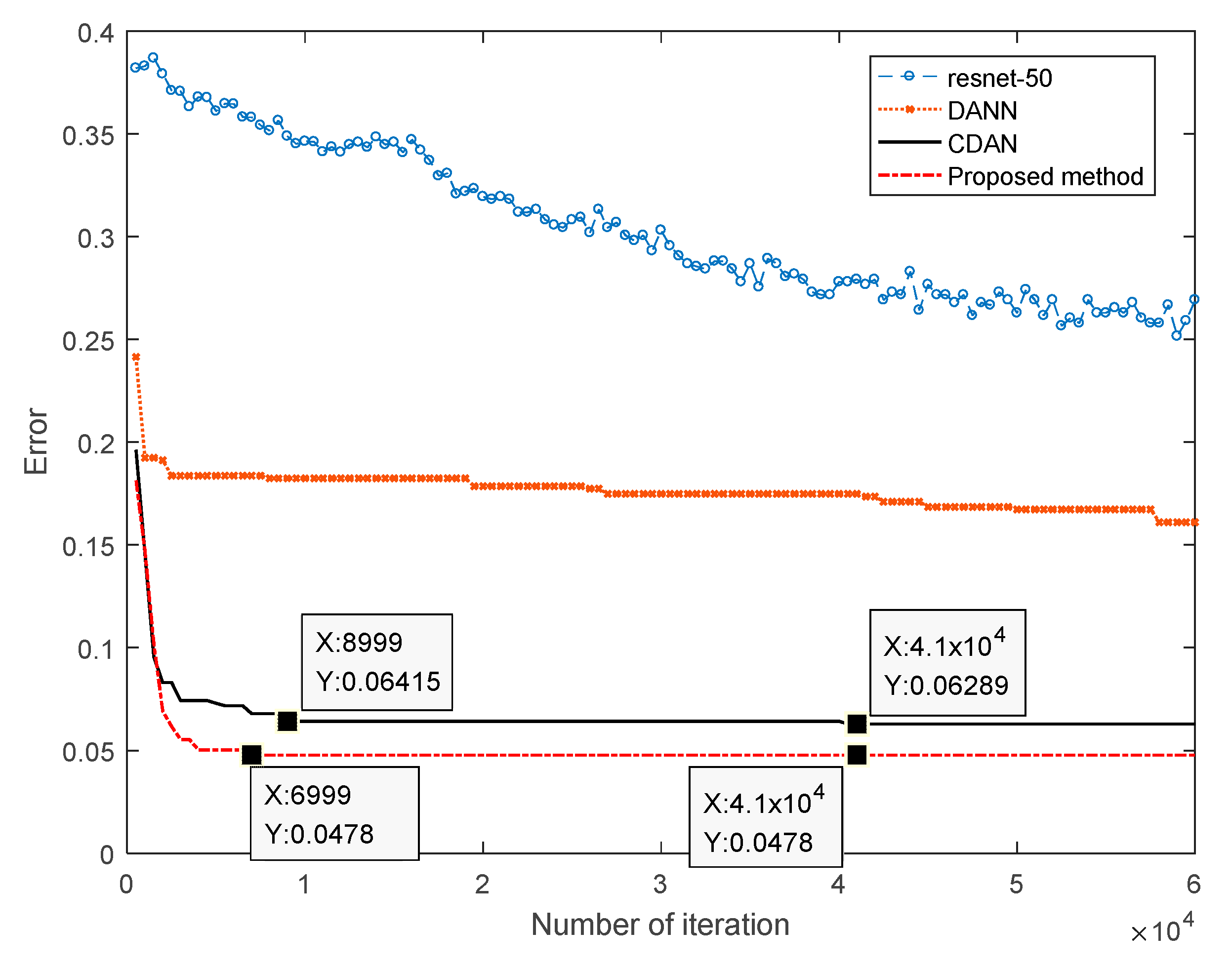
4.2. Comparison of the Convergence Speed

In this section, our proposed method is compared to the ResNet-50, DANN, and CDAN methods to test the performance of its convergence in the test task of A→W using the Office-31 dataset. The results of the comparison are shown in Figure 3.

Figure 3 indicates that the proposed method had the lowest error, while the next best were the CDAN, DANN, and RestNet-50 methods. From the perspective of convergence, the DANN and RestNet-50 methods did not converge after 60,000 iterations. The CDAN method converged after 41,000 iterations, and the proposed method converged after 6999 iterations. When the methods converged, the number of iterations by the proposed method was only about 741. Based on the above analysis presented in Figure 3, the proposed method had faster convergence and fewer errors than the other methods.

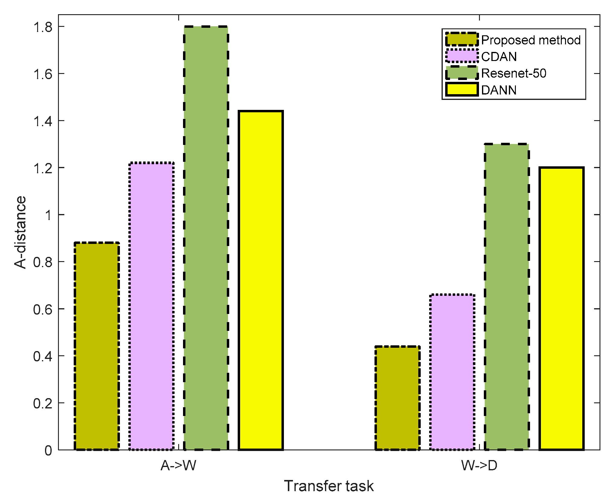
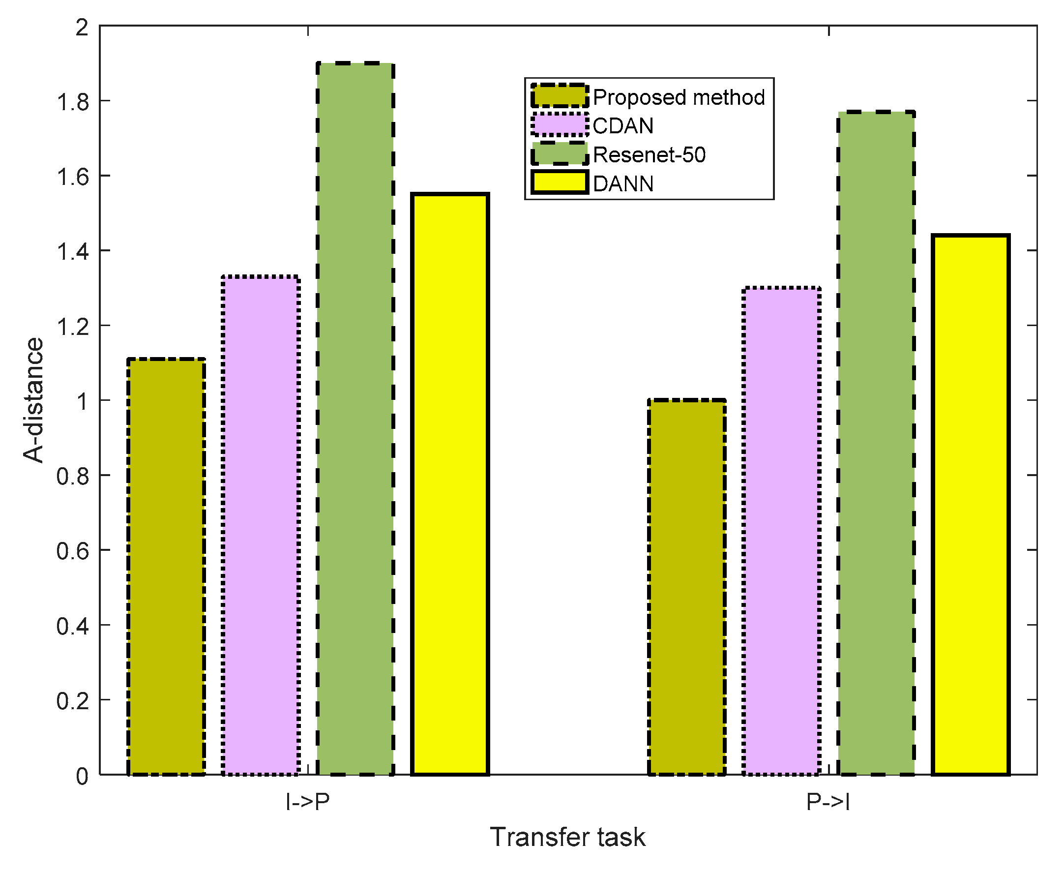
4.3. Comparison of Distribution Discrepancy

In this section, the A-distance [34], which is used by many researchers, is also used to test the performance of different methods in distribution discrepancy. The A-distance can be used to reflect the distribution discrepancy between two datasets. The A-distance can train a binary classifier in the Source and Target domain so that the trained binary classifier can distinguish whether the data come from the Source or Target domain. The A-distance can be expressed as:

$$dis{t}_A=2\left(1-2\epsilon \right),$$

(24)

where $\epsilon$ is the test error of the classifier. The smaller the A-distance, the closer the distance between the Source and Target domains, which were processed by the network in this method. We separately tested for the distribution discrepancy performance of the different methods in the A→W and W→D tasks in the Office-31 dataset, I→P and P→I tasks in the ImageCLEF-DA dataset, and Ar→CI and CI→Ar tasks in the Office-Home dataset. The results are presented in Figure 4, Figure 5 and Figure 6, respectively. In Figure 4, for task A→W, the A-distances of ResNet-50, DANN, CDAN, and the proposed method were 1.8,1.44,1.22, and 0.88, respectively. The proposed method presented the smallest A-distances. In task W→D, the A-distances of ResNet-50, DANN, CDAN, and the proposed method were 1.3,1.2,0.66, and 0.44, respectively. The proposed method again featured the smallest A-distances. In Figure 5 and Figure 6, we can also see that the proposed method retained the smallest A-distances for different tasks. These results imply that the proposed method has the best performance in extracting features.

5. Conclusions

This paper presents the use of spectral normalization in a domain adaption method based on an adversarial network in order to ensure that the gradient satisfies the Lipschitz constraint condition. The results show that this can make the training of domain adaption more stable. The proposed method presents a higher accuracy when compared to other methods based on three different datasets, that is, Office-31, ImageCLEF-DA, and Office-Home. Further, the proposed method exhibits both faster convergence speed and better distribution discrepancy than that achieved by other methods.

References

1. He, K.; Zhang, X.; Ren, S.; Sun, J. Deep residual learning for image recognition. In Proceedings of the IEEE Conference on Computer Vision and Pattern Recognition, Las Vegas, NV, USA, 27–30 June 2016; pp. 770–778. [Google Scholar]
2. Venkateswara, H.; Eusebio, J.; Chakraborty, S.; Panchanathan, S. Deep hashing network for unsupervised domain adaptation. In Proceedings of the IEEE Conference on Computer Vision and Pattern Recognition, Hawaii, HI, USA, 21–26 July 2017; pp. 5018–5027. [Google Scholar]
3. Russakovsky, O.; Deng, J.; Su, H.; Krause, J.; Satheesh, S.; Ma, S.; Huang, Z.; Karpathy, A.; Khosla, A.; Bernstein, M.; et al. Imagenet large scale visual recognition challenge. Int. J. Comput. Vis. 2015, 115, 211–252. [Google Scholar] [CrossRef] [Green Version]
4. Wang, M.; Deng, W. Deep visual domain adaptation: A survey. Neurocomputing 2018, 312, 135–153. [Google Scholar] [CrossRef] [Green Version]
5. Lundervold, A.S.; Lundervold, A. An overview of deep learning in medical imaging focusing on MRI. Z. Med. Phys. 2019, 29, 102–127. [Google Scholar] [CrossRef] [PubMed]
6. Patel, V.M.; Gopalan, R.; Li, R.; Chellappa, R. Visual domain adaptation: A survey of recent advances. IEEE Signal Proc. Mag. 2015, 32, 53–69. [Google Scholar] [CrossRef]
7. Bitarafan, A.; Baghshah, M.S.; Gheisari, M. Incremental evolving domain adaptation. IEEE Trans. Knowl. Data Eng. 2016, 28, 2128–2141. [Google Scholar] [CrossRef]
8. Deng, W.Y.; Lendasse, A.; Ong, Y.S.; Tsang, I.W.; Chen, L.; Zheng, Q. Domain Adaption via Feature Selection on Explicit Feature Map. IEEE Trans. Neural Netw. Learn. Syst. 2018, 30, 1180–1190. [Google Scholar] [CrossRef] [PubMed]
9. Baktashmotlagh, M.; Harandi, M.; Salzmann, M. Distribution-matching embedding for visual domain adaptation. J. Mach. Learn. Res. 2016, 17, 3760–3789. [Google Scholar]
10. Wang, J.; Chen, Y.; Hu, L.; Hu, L.; Peng, X.; Yu, P.S. Stratified transfer learning for cross-domain activity recognition. In Proceedings of the IEEE International Conference on Pervasive Computing and Communications, Athens, Greece, 19–23 March 2018; pp. 1–10. [Google Scholar]
11. Wang, J.; Chen, Y.; Hao, S.; Feng, W.; Shen, Z. Balanced distribution adaptation for transfer learning. In Proceedings of the IEEE International Conference on Data Mining, New Orleans, LA, USA, 18–21 November 2017; pp. 1129–1134. [Google Scholar]
12. Sun, B.; Saenko, K. Deep coral: Correlation alignment for deep domain adaptation. In Proceedings of the European Conference on Computer Vision, Amsterdam, The Netherlands, 8–16 October 2016; pp. 443–450. [Google Scholar]
13. Li, J.; Zhao, J.; Lu, K. Joint Feature Selection and Structure Preservation for Domain Adaptation. In Proceedings of the International Joint Conferences on Artificial Intelligence, New York, NY, USA, 9–16 July 2016; pp. 1697–1703. [Google Scholar]
14. Long, M.; Cao, Y.; Wang, J.; Jordan, M.I. Learning transferable features with deep adaptation networks. In Proceedings of the International Conference on Machine Learning, Lille, France, 6–11 July 2015; pp. 97–105. [Google Scholar]
15. Long, M.; Zhu, H.; Wang, J.; Jordan, M.I. Deep transfer learning with joint adaptation networks. In Proceedings of the International Conference on Machine Learning, Sydney, Australia, 7–9 August 2017; pp. 2208–2217. [Google Scholar]
16. Long, M.; Zhu, H.; Wang, J.; Jordan, M.I. Unsupervised domain adaptation with residual transfer networks. In Proceedings of the Advances in Neural Information Processing Systems, Barcelona, Spain, 5–10 December 2016; pp. 136–144. [Google Scholar]
17. Tzeng, E.; Hoffman, J.; Darrell, T.; Saenko, K. Simultaneous deep transfer across domains and tasks. In Proceedings of the IEEE International Conference on Computer Vision, Santiago, Chile, 7–13 December 2015; pp. 4068–4076. [Google Scholar]
18. Li, Y.; Wang, N.; Shi, J.; Shi, J.; Hou, X.; Liu, J. Adaptive batch normalization for practical domain adaptation. Pattern Recognit. 2018, 80, 109–117. [Google Scholar] [CrossRef]
19. Ganin, Y.; Lempitsky, V. Unsupervised domain adaptation by backpropagation. In Proceedings of the International Conference on Machine Learning, Lille, France, 6–11 July 2015; pp. 1180–1189. [Google Scholar]
20. Goodfellow, I.; Pouget-Abadie, J.; Mirza, M.; Xu, B.; Warde-Farley, D.; Ozair, S.; Courville, A.; Bengio, Y. Generative adversarial nets. In Proceedings of the Advances in Neural Information Processing Systems, Montreal, QC, Canada, 3–8 December 2014; pp. 2672–2680. [Google Scholar]
21. Tzeng, E.; Hoffman, J.; Saenko, K.; Darrell, T. Adversarial discriminative domain adaptation. In Proceedings of the IEEE Conference on Computer Vision and Pattern Recognition, Hawaii, HI, USA, 21–26 July 2017; pp. 7167–7176. [Google Scholar]
22. Long, M.; Cao, Z.; Wang, J.; Jordan, M.I. Conditional adversarial domain adaptation. In Proceedings of the Advances in Neural Information Processing Systems, Montreal, QC, Canada, 3–8 December 2018; pp. 1640–1650. [Google Scholar]
23. Shen, J.; Qu, Y.; Zhang, W.; Yu, Y. Wasserstein distance guided representation learning for domain adaptation. In Proceedings of the AAAI Conference on Artificial Intelligence, New Orleans, LA, USA, 2–7 February 2018; pp. 4058–4065. [Google Scholar]
24. Arjovsky, M.; Chintala, S.; Bottou, L. Wasserstein generative adversarial networks. In Proceedings of the International Conference on Machine Learning, Sydney, Australia, 6–11 August 2017; pp. 214–223. [Google Scholar]
25. Hoffman, J.; Tzeng, E.; Park, T.; Zhu, J.; Isola, P.; Saenko, K.; Efros, A.; Darrell, T. CyCADA: Cycle-Consistent Adversarial Domain Adaptation. In Proceedings of the 35th International Conference on Machine Learning, Vienna, Austria, 10–15 July2018; pp. 1989–1998. [Google Scholar]
26. Liu, M.Y.; Breuel, T.; Kautz, J. Unsupervised image-to-image translation networks. In Proceedings of the Advances in Neural Information Processing Systems, Long Beach CA, USA, 4–9 December 2017; pp. 700–708. [Google Scholar]
27. Cao, Z.; Long, M.; Wang, J.; Jordan, M.I. Partial transfer learning with selective adversarial networks. In Proceedings of the IEEE Conference on Computer Vision and Pattern Recognition, Salt Lake City, UT, USA, 18–22 June 2018; pp. 2724–2732. [Google Scholar]
28. Miyato, T.; Kataoka, T.; Koyama, M.; Yoshida, Y. Spectral normalization for generative adversarial networks. IEEE Trans. Knowl. Data Eng. 2016, 28, 2128–2141. [Google Scholar]
29. Saenko, K.; Kulis, B.; Fritz, M.; Darrell, T. Adapting visual category models to new domains. In Proceedings of the European Conference on Computer Vision, Crete, Greece, 5–11 September 2010; pp. 213–226. [Google Scholar]
30. Paszke, A.; Gross, S.; Massa, F.; Lerer, A.; Bradbury, J.; Chanan, G.; Killeen, T.; Lin, Z.; Gimelshein, N.; Antiga, L.; et al. PyTorch: An imperative style, high-performance deep learning library. In Proceedings of the Advances in Neural Information Processing Systems, Vancouver, BC, Canada, 10–12 December 2019; pp. 8024–8035. [Google Scholar]
31. Sugiyama, M.; Krauledat, M.; MÞller, K.R. Covariate shift adaptation by importance weighted cross validation. J. Mach. Learn. Res. 2007, 8, 985–1005. [Google Scholar]
32. Long, M.; Cao, Y.; Cao, Z.; Wang, J.; Jordan, M.I. Transferable representation learning with deep adaptation networks. IEEE Trans. Pattern Anal. 2019, 41, 3071–3085. [Google Scholar] [CrossRef] [PubMed]
33. You, K.; Wang, X.; Long, M.; Jordan, M.I. Towards Accurate Model Selection in Deep Unsupervised Domain Adaptation. In Proceedings of the International Conference on Machine Learning, Boca Raton, FL, USA, 16–19 December 2019; pp. 7124–7133. [Google Scholar]
34. Ben-David, S.; Blitzer, J.; Crammer, K.; Kulesza, A.; Pereira, F.; Vaughan, J.W. A theory of learning from different domains. Mach. Learn. 2010, 79, 151–175. [Google Scholar] [CrossRef] [Green Version]
Figure 1. Network structure of the conditional adversarial domain adaptation (CDAN). (a) Network structure in a low-dimensional scenario; (b) Network structure in a high-dimensional scenario.
Information 11 00068 g001
Figure 2. The network structure of the proposed method.
Information 11 00068 g002
Figure 3. Relationship between the number of iterations and errors for the different methods.
Information 11 00068 g003
Figure 4. Distribution discrepancy of different methods for the Office-31 dataset.
Information 11 00068 g004
Figure 5. Distribution discrepancy of the different methods for the ImageCLEF-DA dataset.
Information 11 00068 g005
Figure 6. Distribution discrepancy of different methods for the Office-Home dataset.
Information 11 00068 g006