Kernel-Based Ensemble Learning in Python

Abstract

We propose a new supervised learning algorithm for classification and regression problems where two or more preliminary predictors are available. We introduce KernelCobra, a non-linear learning strategy for combining an arbitrary number of initial predictors. KernelCobra builds on the COBRA algorithm introduced by Biau et al. (2016), which combined estimators based on a notion of proximity of predictions on the training data. While the COBRA algorithm used a binary threshold to declare which training data were close and to be used, we generalise this idea by using a kernel to better encapsulate the proximity information. Such a smoothing kernel provides more representative weights to each of the training points which are used to build the aggregate and final predictor, and KernelCobra systematically outperforms the COBRA algorithm. While COBRA is intended for regression, KernelCobra deals with classification and regression. KernelCobra is included as part of the open source Python package Pycobra (0.2.4 and onward), introduced by Srinivasa Desikan (2018). Numerical experiments were undertaken to assess the performance (in terms of pure prediction and computational complexity) of KernelCobra on real-life and synthetic datasets.

1. Introduction

In the fields of machine learning and statistical learning, ensemble methods consist of combining several estimators (or predictors) to create a new, superior estimator. Ensemble methods (also known as aggregation in the statistical literature) have attracted tremendous interest in recent years, and for a few problems, are considered state-of-the-art techniques, as discussed by Bell and Koren [1]. There is a wide variety of ensemble algorithms (some of which are discussed in Dietterich [2], Giraud [3] and Shalev-Shwartz and Ben-David [4]), with a crushing majority devoted to linear or convex combinations.

In this paper we propose a non-linear way of combining estimators, adding to a streamline of works pioneered by Mojirsheibani [5]. Our method (KernelCobra) extends the COBRA (standing for combined regression alternative) algorithm introduced by Biau et al. [6]. The COBRA algorithm is motivated by the idea that non-linear, data-dependent techniques can provide flexibility not offered by existing (linear) ensemble methods. By using information of proximity between the training data and predictions on test data, training points are collected to perform the aggregate. The COBRA algorithm selects training points by checking whether the proximity is less than a data dependant threshold $ϵ$, resulting in a binary decision (either keep the point or discard it). The KernelCobra algorithm introduced in the present paper aims to smoothen this data point selection process by introducing a kernel-based method to assigning weights to various points in the collective. The only weights that points could take in the COBRA algorithm were a discrete set between 0 and 1, whereas our smoothed scheme will span real values between 0 and 1. A python implementation of KernelCobra is provided in the python package Pycobra, introduced and described by Guedj and Srinivasa Desikan [7]. We found in numerical experiments that KernelCobra consistently outperforms the original COBRA algorithm in a variety of situations.

The paper is organised as follows. Section 2 discusses related work and Section 3 introduces the ideas leading to KernelCobra. Section 4 presents the actual implementations of KernelCobra in the pycobra Python library. Section 5 illustrates the performance (both in prediction accuracy and computational complexity) on real-life and synthetic datasets, along with comparable aggregation techniques. Section 6 presents avenues for future work.

2. Related Work

Our algorithm is inspired by the work of Biau et al. [6] which introduced the COBRA algorithm. COBRA itself is inspired by the seminal work by Mojirsheibani [5], where the idea of using consensus between machines to create an aggregate was first discussed. Our algorithm KernelCobra is a strict generalisation of COBRA.

In a work parallel to ours, the idea of using the distance between points in the output space is also explored by Fischer and Mougeot [8], where weights are assigned to points based on proximity of the prediction in the output space and the training data. However, the method employed (which will now be referred to as MixCobra) also uses the input data while constructing the aggregate. While it is true that more data-dependant information might improve the quality of the aggregate, we argue that in cases with high-dimensional input data, proximity between points will not add much useful information. Computing distance metrics in high dimensions is a computational challenge, which in our view, could undermine the statistical performance (see [9] for discussion). While using both input and output information might provide satisfactory results in lower dimensions, non-linear ensemble learning algorithms arguably perform particularly well in high dimensions, as they are not affected by the dimension of the input space. This edge is lost in the MixCobra method.

KernelCobra overcomes this problem by only considering proximity of data points in the prediction space, allowing to perform faster calculations. This makes KernelCobra a promising candidate for high dimensional learning problems: as a matter of fact, KernelCobra is not affected at all by the curse of dimensionality, with the complexity only increasing with the number of preliminary estimators.

In a recent work, the original COBRA algorithm (as implemented by the pycobra Python library; see Guedj and Srinivasa Desikan [7]) was successfully adapted by Guedj and Rengot [10] to perform image denoising. The authors report that the COBRA-based denoising algorithm significantly outperforms most state-of-the-art denoising algorithms on a benchmark dataset, calling for the broadcasting of non-linear ensemble methods in computer vision and image processing communities.

3. KernelCobra: A Kernelized Version of COBRA

Throughout this section, assume that we are given a training sample $D_n$ = $({\mathbf{X}}_1,Y_1),\dots ,({\mathbf{X}}_n,Y_n)$ of i.i.d. copies of $(\mathbf{X},Y)\in {\mathbb{R}}^d\times \mathbb{R}$ (with the notation $\mathbf{X}=(X_1,\dots ,X_d))$. Assume that $\mathbb{E}{Y}^2$$<\infty$. The space ${\mathbb{R}}^d$ is equipped with the standard euclidean metric. Our goal is to consistently estimate the regression function $r^{🞰}\left(\mathbf{x}\right)$ = $\mathbb{E}\left[Y\right|\mathbf{X}=\mathbf{x}]$, for some new query point $\mathbf{x}\in R^d$, using the data $D_n$.

To begin with, the original data set $D_n$ is split into two data sequences $D_k=({\mathbf{X}}_1,Y_1),\dots ,({\mathbf{X}}_k,Y_k)$ and $D_{\ell }=({\mathbf{X}}_{k+1},Y_{k+1}),\dots ,({\mathbf{X}}_n,Y_n)$, with $\ell =n-k\ge 1$. For ease of notation, the elements of $D_{\ell }$ are renamed $({\mathbf{X}}_1,Y_1),\dots ,({\mathbf{X}}_l,Y_l)$, similar to the notation used by Biau et al. [6].

Now, suppose that we are given a collection of $M\ge 1$ competing estimators (referred to as machines from now on) $r_{k,1},\dots ,r_{k,M}$ to estimate $r^{🞰}$. These preliminary machines are assumed to be generated using only the first sub-sample $D_k$. In all practical scenarios, machines can be any machine learning algorithm, from classical linear regression all the way up to a deep neural network, including naive Bayes, decision trees, penalised regression, random forest, k-nearest neighbours and so on. These machines have no restrictions in their nature: they can be parametric or nonparametric. The only condition is that each of these machines $m=1,\dots ,M$ is able to provide an estimation $r_{k,m}\left(\mathbf{x}\right)$ of $r^{🞰}\left(\mathbf{x}\right)$ on the basis of $D_k$ alone. Let us stress here that the number of machines M is fixed.

Let us recall the COBRA algorithm, introduced by Biau et al. [6]: for any query point $\mathbf{x}\in {\mathbb{R}}^d$, the aggregated estimator COBRA is given by

$$T_n\left({\mathbf{r}}_k\left(\mathbf{x}\right)\right)=\sum _{i=1}^{\ell }{W}_{n,i}\left(\mathbf{x}\right)Y_i,$$

(1)

where the random weights are given by Biau et al. [6] (Equation (2.1))

$$W_{n,i}\left(\mathbf{x}\right)=\frac{{\mathbf{1}}_{{\cap }_{m=1}^M\left\{\right|r_{k,m}\left({\mathbf{X}}_i\right)-r_{k,m}\left(\mathbf{x}\right)|\le ϵ\}}}{{\displaystyle \sum {}_{j=1}^{\ell }{\mathbf{1}}_{{\cap }_{m=1}^M\left\{\right|r_{k,m}\left({\mathbf{X}}_j\right)-r_{k,m}\left(\mathbf{x}\right)|\le ϵ\}}}},$$

(2)

where ${\mathbf{1}}_A$ denotes the indicator function of a set A, given by

$${\mathbf{1}}_A:\mathbf{x}\mapsto \left\{\begin{array}{c}1\mathrm{if}\mathbf{x}\in A,\hfill \\ 0\mathrm{if}\mathrm{not}.\hfill \end{array}\right.$$

This aggregation strategy operates in a nonlinear way with respect to the preliminary machines, by aggregating outputs only.

The (possibly data-dependent) threshold parameter $ϵ>0$ serves to discard points from the initial sample for which at least one prediction made by a machine is considered too far from the prediction made on the new query point: this then sets this point’s weight to zero. This threshold parameter needs to be finely tuned (using cross-validation in the initial COBRA algorithm). One motivation for introducing KernelCobra is to attenuate this dependence on a problem-dependent threshold parameter.

In addition, the rather bumpy behaviour of the weights in (2) (they can only take finite values in the set $\{0,1/\ell ,1/(\ell -1),\dots ,1\}$) only allows for restricted expressivity. Another motivation for introducing KernelCobra is to allow for continuous values in $(0,1)$, and hence, it increases flexibility. Last but not least, the more generic formulation of KernelCobra will yield better performance than COBRA’s, as illustrated in Section 5.

As a gentle start, we now introduce a version of KernelCobra with the Euclidean distance $d_{\epsilon }$ and an exponential form of the weights—these will be eventually generalised.

Given the collection of basic machines ${\mathbf{r}}_k=(r_{k,1},\dots ,r_{k,M})$, we define the aggregated estimator for any $\mathbf{x}\in {\mathbb{R}}^d$ as in (1),

$$T_n\left({\mathbf{r}}_k\left(\mathbf{x}\right)\right)=\sum _{i=1}^{\ell }{W}_{n,i}\left(x\right)Y_i,$$

(3)

where the random weights $W_{n,i}\left(\mathbf{x}\right)$ are now given by

$$W_{n,i}\left(\mathbf{x}\right)=\frac{exp\left\{-\lambda \sum {}_{m=1}^M{d}_{\epsilon }(r_{k,m}\left({\mathbf{X}}_i\right),r_{k,m}\left(\mathbf{x}\right))\right\}}{{\displaystyle \sum {}_{j=1}^{\ell }exp\left\{-\lambda \sum {}_{m=1}^M{d}_{\epsilon }(r_{k,m}\left({\mathbf{X}}_j\right),r_{k,m}\left(\mathbf{x}\right))\right\}}}.$$

(4)

The hyperparameter $\lambda >0$ acts as a temperature parameter, to adjust the level of fit to data, and will be optimised in numerical experiments using cross-validation. Let us stress here that $d_{\epsilon }(a,b)$ denotes the Euclidean distance between any two points $a,b\in \mathbb{R}$. In (4), this serves as a way to measure the proximity or coherence between predictions on training data and predictions made for the new query point, across all machines.

This form (4) is more smooth than the form introduced in the COBRA algorithm [6] and is reminiscent of exponential weights. The aggregated estimator in (1) with weights defined in (4) is called KernelCobra.

A more generic form is given by

$$W_{n,i}\left(\mathbf{x}\right)=\frac{\sum {}_{m=1}^{M}K(r_{k,m}\left({\mathbf{X}}_i\right),r_{k,m}\left(\mathbf{x}\right))}{{\displaystyle \sum {}_{j=1}^{\ell }\sum {}_{m=1}^{M}K(r_{k,m}\left({\mathbf{X}}_j\right),r_{k,m}\left(\mathbf{x}\right))}},$$

(5)

where K denotes a kernel used to capture the proximity between predictions on training and query data, across machines. The aggregated estimator in (1) with weights defined in (5) is called general KernelCobra.

Rather than a threshold to keep or discard data point i in the weights (as with the initial COBRA algorithms with weights defined in Equation (2)), its influence is now always considered, by a measure of how preliminary machines predict outcomes for the new query point which are close to the predictions made for point i. In other words, a data point i will have more influence on the aggregated estimator (its weight will be higher) if machines predict similar outcomes for i and the new query point. Let us stress again here that KernelCobra, as the initial COBRA algorithm, aggregates machines in a non-linear way: the aggregated estimator in (1) is a weighted combination of observed outputs$Y_i$s, not of initial machines (which serve to build the weights). As such, it is fairly different from most aggregation schemes which form linear combinations of machines’ outcomes.

Note also that computing the weights defined in (4) and (5) involves elementary computations over scalars (each machine’s prediction over the training sample and the new query point) rather than d-dimensional vectors. As highlighted above, both versions of KernelCobra avoid the curse of dimensionality.

General KernelCobra allows for the use of any kernel which might be preferred by practitioners—it is the generic version of our algorithm. In practice, we have found that the KernelCobra defined with weights in (4) provides interesting empirical results, and is more interpretable. We thus provide both versions, as they express a trade-off between generality and ease of interpretation and use.

The remainder of this section is devoted to two interesting byproducts of our approach, to the unsupervised setting and for classification.

3.1. The Unsupervised Setting

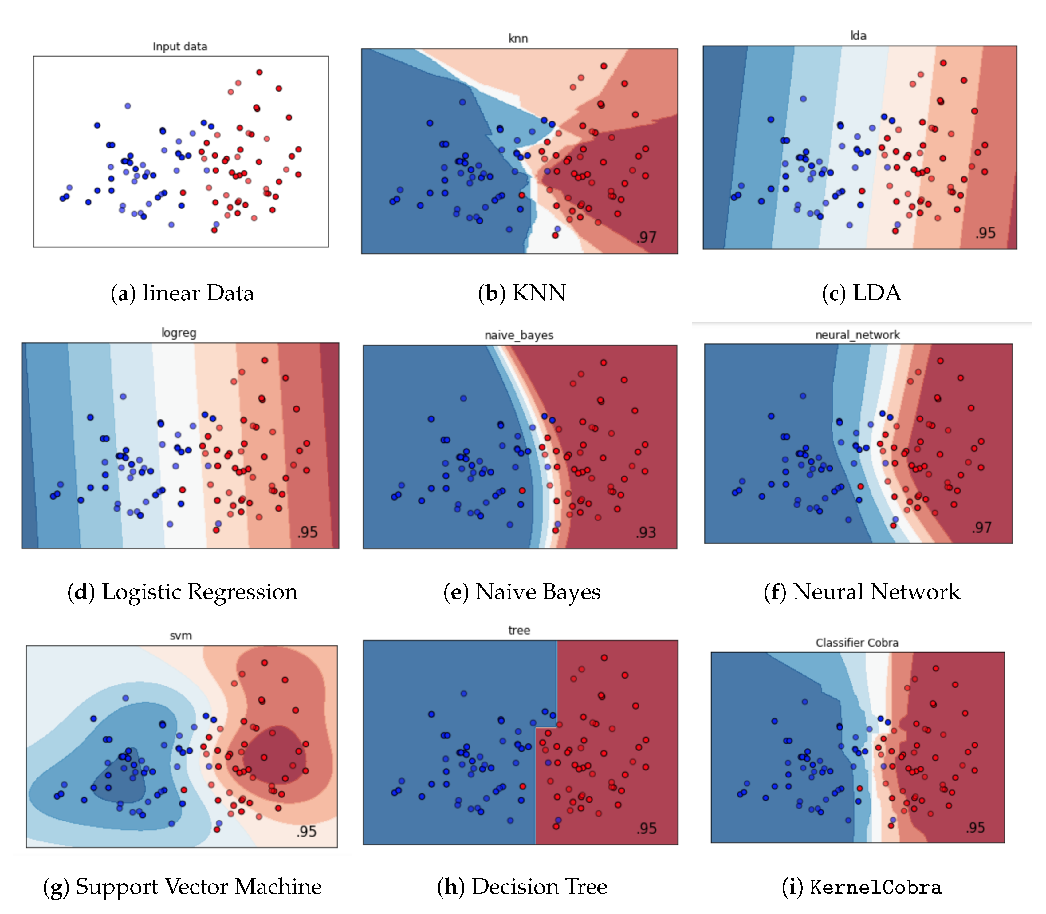
As COBRA and KernelCobra are non-linear aggregation methods, the final estimator is a weighted combination of observed outputs $Y_i$s. We can turn our approach to a more classical linear aggregation scheme, to the notable point that none of the approaches depend on $Y_i$s, allowing us to consider the unsupervised setting. This differs from classical linear or convex aggregation methods such as exponential weights: the weights depend on a measure of performance such as an empirical risk, which will involve $Y_i$s.

We can now throw away all $Y_j$s for $j=1,\dots ,\ell$, and we propose the following estimator for any new query point $\mathbf{x}\in {\mathbb{R}}^d$:

$$T_n\left({\mathbf{r}}_k\left(\mathbf{x}\right)\right)=\sum _{i=1}^{\ell }{W}_{n,i}\left(\mathbf{x}\right)\sum _{m=1}^M{r}_{k,m}\left({\mathbf{X}}_i\right){\tilde{W}}_{n,m}.$$

(6)

Our first set of weights ${\left(W_{n,i}\left(\mathbf{x}\right)\right)}_{i=1}^{\ell }$ is given by (4) or (5), and serves to weigh data points. Our second set of weights ${\left({\tilde{W}}_{n,m}\right)}_{m=1}^M$ used to aggregate the predictions of each machine, can be any sequence of weights summing up to 1, and serves to weigh machines.

In other words, once the machines have been trained (either in a supervised setting using the outputs in subsample $D_k$, or in an unsupervised setting by discarding all outputs across the dataset D), the estimator defined in (6) no longer needs outputs from the second half of the dataset $D_{\ell }$, thereby extending to semi-supervised and unsupervised settings, further illustrating the flexibility of our approach.

3.2. Classification

Non-linear aggregation of classifiers has been studied by Mojirsheibani [5] and Mojirsheibani [11] (where a kernel is also used to smoothen the point selection process). The papers Mojirsheibani [12] and Balakrishnan and Mojirsheibani [13] focus on using the misclassification error to build the aggregate. Here we provide a simple extension of our approach to classification.

For binary classification ($\mathcal{Y}=\{0,1\}$), the combined classifier is given by

$$C_n\left(\mathbf{x}\right)=\left\{\begin{array}{cc}1,\hfill & \mathrm{if}{\sum }_{i=1}^{\ell }{Y}_i{W}_{n,i}\left(\mathbf{x}\right)\ge \frac{1}{2},\hfill \\ 0,\hfill & \mathrm{otherwise}.\hfill \end{array}\right.$$

(7)

The weights can be chosen as (4) or (5).

We also provide a combined classifier for the multi-class setting: let us assume that $\mathcal{Y}$ is a finite discrete set of classes,

$$C_n\left(\mathbf{x}\right)=\underset{k\in \mathcal{Y}}{argmax}\sum _{i=1}^{\ell }{\mathbf{1}}_{\{Y_i=k\}}{W}_{n,i}\left(\mathbf{x}\right).$$

(8)

To conclude this section, let us mention that Biau et al. [6] (Theorem 2.1) proved that the combined estimator with weights chosen as in the initial COBRA algorithm (2) enjoys an oracle guarantee: the average quadratic loss of the estimator is upper bounded by the best (lowest) quadratic loss of the machines up to a remainder term of magnitude $\mathcal{O}\left({\ell }^{-\frac{2}{M+2}}\right)$. This result is remarkable, as it does not involve the ambient dimension d but rather the (fixed) number of machines M. We focus in the present paper on the introduction of KernelCobra and its variants, and its implementation in Python (detailed in the next section). We leave for a future work the extension of Biau et al. [6]’s theoretical results.

4. Implementation

All new algorithms described in the present paper are implemented in the Python library pycobra (from version 0.2.4 and onward); we refer to Guedj and Srinivasa Desikan [7] for more details.

The python library pycobra can be installed via pip using the command pip install pycobra. The PyPi page for pycobra is https://pypi.org/project/pycobra/. The code for pycobra is open source and can be found on GitHub at https://github.com/bhargavvader/pycobra. The documentation for pycobra is hosted at https://modal.lille.inria.fr/pycobra/.

We describe the general KernelCobra algorithm in Algorithm 1.

Algorithm 1: General KernelCobra

KernelCobra is implemented as part of the KernelCobra class in the pycobra package. The estimator is scikit-learn compatible (see Pedregosa et al. [14]), and works similarly to the other estimators provided in the pycobra package. The only hyperparameter accepted in creating the object is a random state object.

The pred method implements the algorithm described in Algorithm 1, and the predict method serves as a wrapper for the pred method to ensure it is scikit-learn compatible. It should be noted that the predict method can be customised to pass any user-defined kernel (along with parameters), as suggested by (5). The default behaviour of the predict method is set to use the weights defined in (4).

Similarly to the other estimators provided in pycobra, KernelCobra can be used with the Diagnostics and Visualisation classes, which are used for debugging and visualising the model. Since it abides the scikit-learn ecosystem, one can use either GridSearchCV or the Diagnostics class to tune the parameters for KernelCobra (such as the temperature parameter).

The default regression machines used for KernelCobra are the scikit-learn implementations of lasso, random forest, decision trees and ridge regression. This is merely an editorial choice to have the algorithm up and ready immediately, but let us stress here that one can provide any estimator using the load_machine method, with the only constraints being that it must be trained on $D_k$, and that it has a valid predict method.

We also provide the pseudo-code for the variant of KernelCobra in semi-supervised or unsupervised settings defined by (6) (Algorithm 2), along with the variant for multi-class classification defined by (8) (Algorithm 3).    

Algorithm 2:KernelCobra in the unsupervised setting

Algorithm 3:KernelCobra for classification

To conclude this section, let us mention that the complexity of all presented algorithms is $\mathcal{O}\left(M\ell \right)$ as we loop over all data points in the subsample $D_{\ell }$ and over all machines.

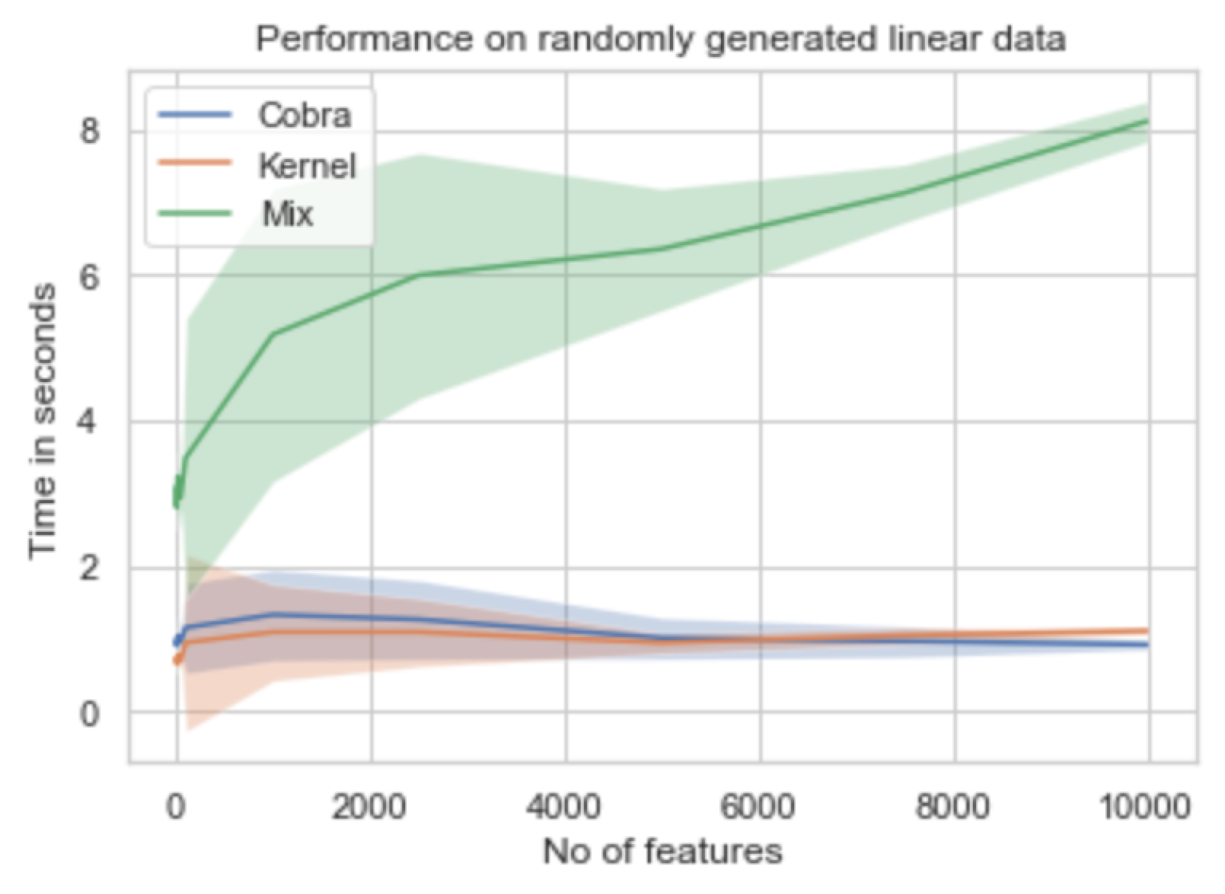
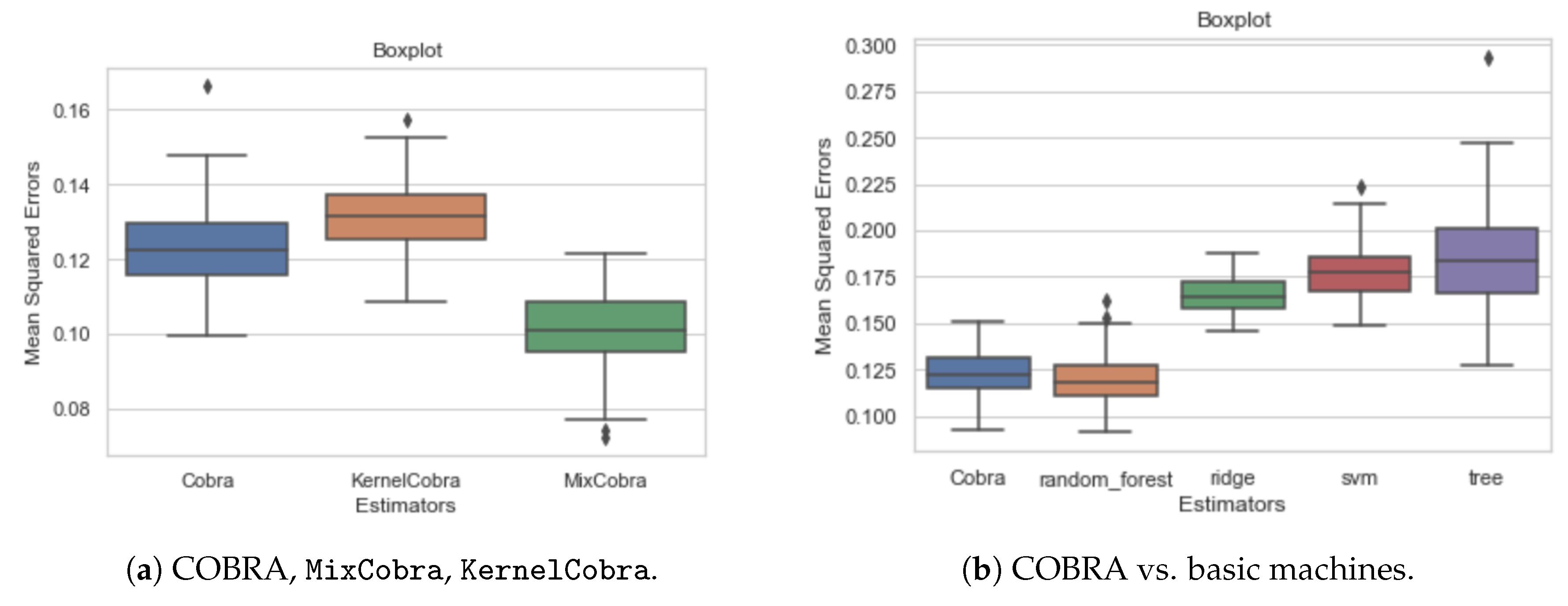
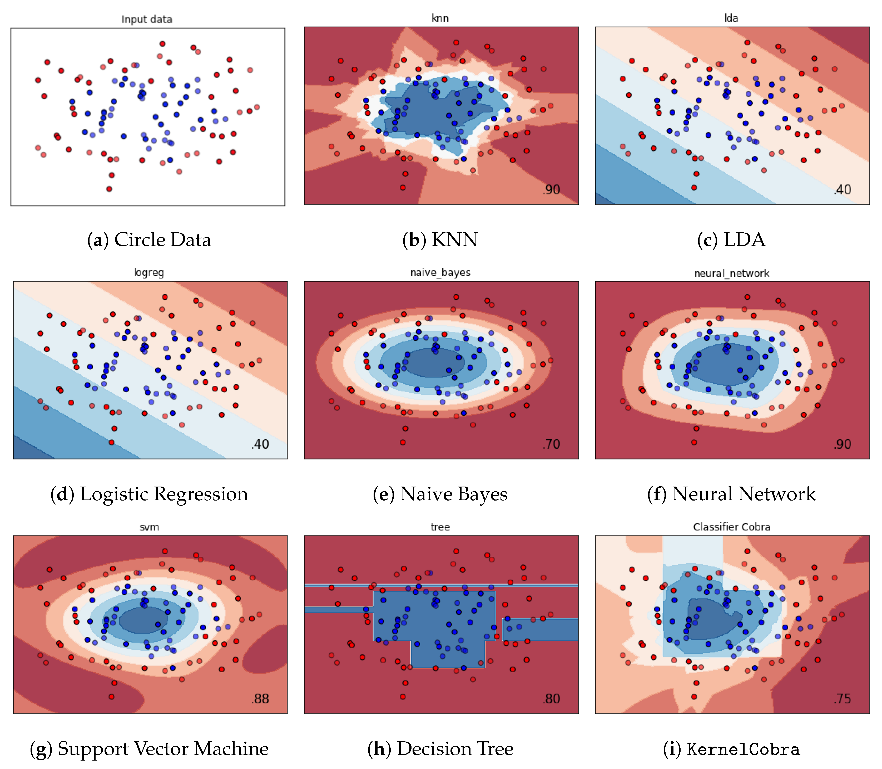
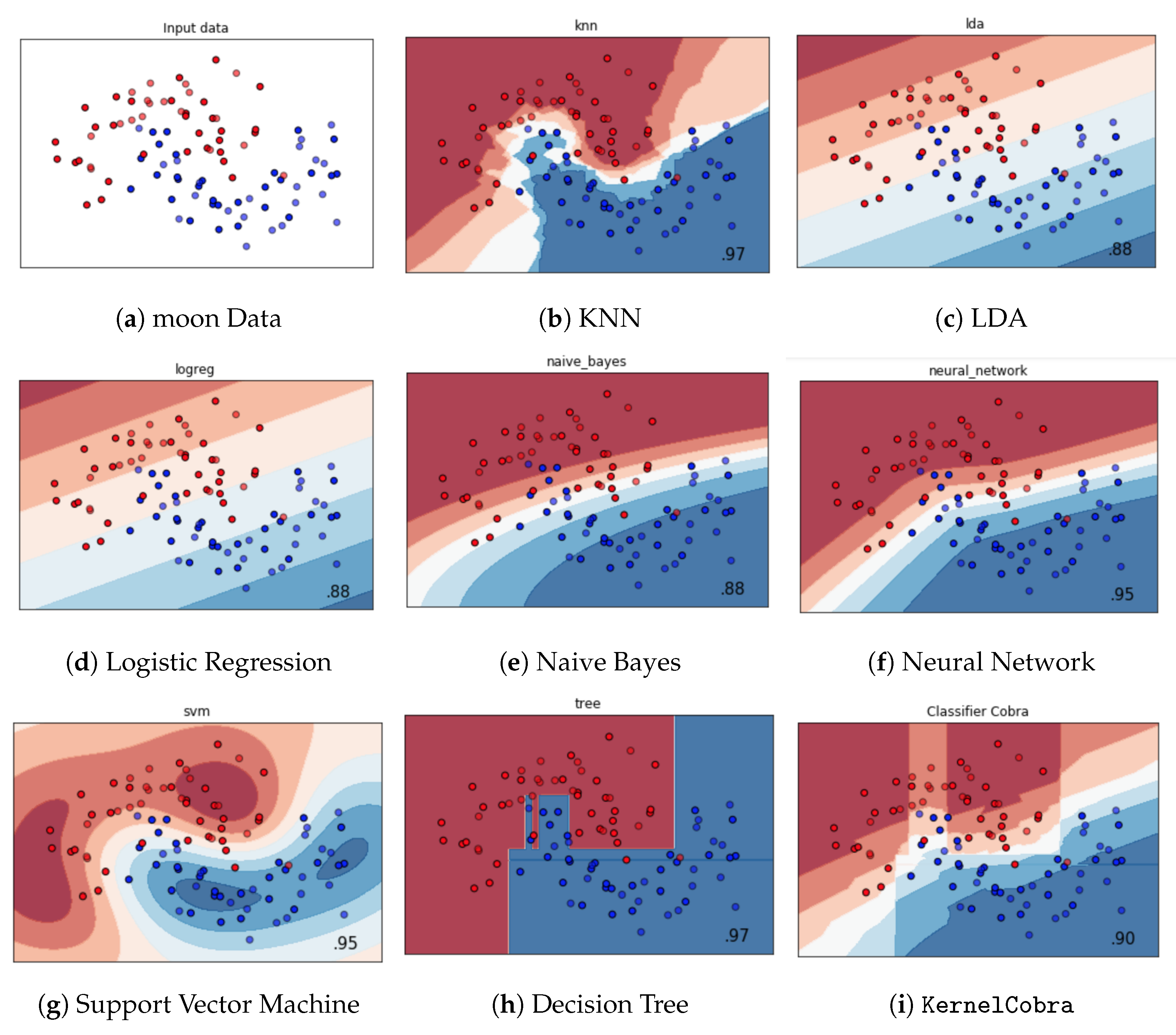
5. Numerical Experiments

We have conducted numerical experiments to assess the merits of KernelCobra in terms of statistical performance, and computational cost. We compare pythonic implementations of KernelCobra, MixCobra, the original COBRA algorithm as implemented by pycobra and the default scikit-learn machines used to create our aggregate.

We test our method on four synthetic data-sets and two real world data-sets, and report statistical accuracy and CPU-timing. The synthetic datasets are generated using scikit-learn’s make-regression, make-friedman1 and make-sparse-uncorrelated functions. The two real world datasets are the Boston Housing dataset (https://www.cs.toronto.edu/~delve/data/boston/bostonDetail.html), and the Diabetes dataset (https://archive.ics.uci.edu/ml/datasets/diabetes).

Table 1. For each estimator and each dataset (names point to datasets URLs), we report the mean root mean square error (RMSE—along with standard deviation) over 100 independent runs. Bold numbers indicate the best method for each dataset.

	Gaussian	Sparse	Diabetes	Boston	Linear	Friedman
random-forest	12,266.640297	3.35474	2924.12121	18.47003	0.116743	5.862687
	(1386.2011)	(0.3062)	(415.4779)	(4.0244)	(0.0142)	(0.706)
ridge	491.466644	1.23882	2058.08145	13.907375	0.165907	6.631595
	(201.110142)	(0.0311)	(127.6948)	(2.2957)	(0.0101)	(0.2399)
svm	1699.722724	1.129673	8984.301249	74.682848	0.178525	7.099232
	(441.8619)	(0.0421)	(236.8372)	(114.9571)	(0.0155)	(0.3586)
tree	22,324.209936	6.304297	5795.58075	32.505575	0.185554	11.136161
	(3309.8819)	(0.9771)	(1251.3533)	(14.2624)	(0.0246)	(1.73)
Cobra	1606.830549	1.951787	2506.113231	16.590891	0.12352	5.681025
	(651.2418)	(0.5274)	(440.1539)	(8.0838)	(0.0109)	(1.3613)
KernelCobra	488.141132	1.11758	2238.88967	12.789762	0.113702	4.844789
	(189.9921)	(0.1324)	(1046.0271)	(9.3802)	(0.0089)	(0.5911)
MixCobra	683.645028	1.419663	2762.95792	16.228564	0.104243	5.068543
	(196.7856)	(0.1292)	(512.6755)	(12.7125)	(0.0104)	(0.6058)

Gaussian (https://scikit-learn.org/stable/modules/generated/sklearn.datasets.make_regression.html#sklearn.datasets.make_regression); Sparse (https://scikit-learn.org/stable/modules/generated/sklearn.datasets.make_sparse_uncorrelated.html#sklearn.datasets.make_sparse_uncorrelated); Diabetes (https://archive.ics.uci.edu/ml/datasets/diabetes; Boston (https://www.cs.toronto.edu/~delve/data/boston/bostonDetail.html; Linear (https://scikit-learn.org/stable/modules/generated/sklearn.datasets.make_regression.html#sklearn.datasets.make_regression); Friedman (https://scikit-learn.org/stable/modules/generated/sklearn.datasets.make_friedman1.html#sklearn.datasets.make_friedman1).

wraps up our results for statistical accuracy and establishes KernelCobra as a promising new kernel-based ensemble learning algorithm. KernelCobra achieves the smallest mean error on four datasets (Gaussian, Sparse, Boston, Friedman) out of six, with the ridge algorithm and MixCobra winning in the other two. Out of these six classical datasets, KernelCobra systematically outperforms the initial COBRA algorithm.

Figure 1 compares the computational costs of the original COBRA, MixCobra and KernelCobra. As both COBRA and KernelCobra do not use the input data, they do not suffer from an increase of data dimensionality and significantly outperform MixCobra. A salient fact is that the computational complexity of KernelCobra does not increase with the number of features.

The pycobra package also offers a visualisation suite which gives QQ-plots, boxplots of errors and comparisons between the predictions of machines and the aggregate, along with the true values. We report a sample of those outputs in Figure 2.

Last but not least, we provide a sample of decision boundaries for the classification variant of KernelCobra on three datasets, in Figure 3, Figure 4 and Figure 5. These three datasets are scikit-learn generic datasets for classification—linearly-separable, make-moons and make-circles. The nature of these datasets provides us a way to visualise how ClassifierCobra classifies with regard to the default classifiers used.

Some notes about the nature of the experiments and the performance: KernelCobra is the best performing machine for four out of six datasets. These values were achieved using an optimally derived bandwidth parameter for that dataset. This was calculated using the optimal-kernelbandwidth function in the Diagnostics class of the pycobra package. The default bandwidth values do not perform as well, and if we further fine-tune the bandwidth value, we would get potentially better results. MixCobra has similar tunable parameters which affect its performance, but takes significantly longer, as there are three parameters to tune. We used the default range of parameters to test before choosing optimal parameters for both KernelCobra and MixCobra in the results displayed.

When considering both the CPU timing to find optimal parameters and the statistical performance, KernelCobra outperforms the initial COBRA algorithm.

6. Conclusions and Future Work

The COBRA algorithm from Biau et al. [6] established a nonlinear aggregation method with theoretical guarantees and competitive numerical performance. In the present paper, we introduced a generalisation of the COBRA algorithm—called KernelCobra—to make it more flexible and user-friendly, and increase its performance on a wider range of problems (classification and regression—supervised, semi-supervised or unsupervised). KernelCobra delivers a kernel-based ensemble learning algorithm which is versatile, computationally cheap and flexible. All variants of KernelCobra ship as part of the pycobra Python library introduced by Guedj and Srinivasa Desikan [7] (from version 0.2.4), and are designed to be used in a scikit-learn environment. We will conduct, in future work, a theoretical analysis of the kernelised COBRA algorithm to complete the theory provided by Biau et al. [6].

References

1. Bell, R.M.; Koren, Y. Lessons from the Netflix prize challenge. ACM SIGKDD Explor. Newsl. 2007, 9, 75–79. [Google Scholar] [CrossRef]
2. Dietterich, T.G. Ensemble methods in machine learning. In International Workshop on Multiple Classifier Systems; Springer: Berlin, Germany, 2000; pp. 1–15. [Google Scholar]
3. Giraud, C. Introduction to High-Dimensional Statistics; CRC Press: Boca Raton, FL, USA, 2014. [Google Scholar]
4. Shalev-Shwartz, S.; Ben-David, S. Understanding Machine Learning: From Theory to Algorithms; Cambridge University Press: Cambridge, UK, 2014. [Google Scholar]
5. Mojirsheibani, M. Combining classifiers via discretization. J. Am. Stat. Assoc. 1999, 94, 600–609. [Google Scholar] [CrossRef]
6. Biau, G.; Fischer, A.; Guedj, B.; Malley, J.D. COBRA: A combined regression strategy. J. Multivar. Anal. 2016, 146, 18–28. [Google Scholar] [CrossRef]
7. Guedj, B.; Srinivasa Desikan, B. Pycobra: A Python Toolbox for Ensemble Learning and Visualisation. J. Mach. Learn. Res. 2018, 18, 1–5. [Google Scholar]
8. Fischer, A.; Mougeot, M. Aggregation using input–output trade-off. J. Stat. Plan. Inference 2019, 200, 1–19. [Google Scholar] [CrossRef] [Green Version]
9. Steinbach, M.; Ertöz, L.; Kumar, V. The challenges of clustering high dimensional data. In New Directions in Statistical Physics; Springer: Berlin, Germany, 2004; pp. 273–309. [Google Scholar]
10. Guedj, B.; Rengot, J. Non-linear aggregation of filters to improve image denoising. arXiv 2019, arXiv:1904.00865. [Google Scholar]
11. Mojirsheibani, M. A kernel-based combined classification rule. Stat. Probab. Lett. 2000, 48, 411–419. [Google Scholar] [CrossRef]
12. Mojirsheibani, M. An almost surely optimal combined classification rule. J. Multivar. Anal. 2002, 81, 28–46. [Google Scholar] [CrossRef] [Green Version]
13. Balakrishnan, N.; Mojirsheibani, M. A simple method for combining estimates to improve the overall error rates in classification. Comput. Stat. 2015, 30, 1033–1049. [Google Scholar] [CrossRef]
14. Pedregosa, F.; Varoquaux, G.; Gramfort, A.; Michel, V.; Thirion, B.; Grisel, O.; Blondel, M.; Prettenhofer, P.; Weiss, R.; Dubourg, V.; et al. Scikit-learn: Machine learning in Python. J. Mach. Learn. Res. 2011, 12, 2825–2830. [Google Scholar]
Figure 1. CPU timing for building the initial COBRA, MixCobra and KernelCobra estimators. Each line is an average over 100 independent runs, and shaded areas show standard deviations.
Information 11 00063 g001
Figure 2. Boxplot of errors over 100 independent runs.
Information 11 00063 g002
Figure 3. Decision boundaries of base classifiers and KernelCobra on the circle dataset.
Information 11 00063 g003
Figure 4. Decision boundaries of base classifiers and KernelCobra on the moon dataset.
Information 11 00063 g004
Figure 5. Decision boundaries of base classifiers and KernelCobra on the linear dataset.
Information 11 00063 g005