A New Method for Refined Recognition for Heart Disease Diagnosis Based on Deep Learning

Abstract

The proper evaluation of heart health requires professional medical experience. Therefore, in clinical diagnosis practice, the development direction is to reduce the high dependence of the diagnosis process on medical experience and to more effectively improve the diagnosis efficiency and accuracy. Deep learning has made remarkable achievements in intelligent image analysis technology involved in the medical process. From the aspect of cardiac diagnosis, image analysis can extract more profound and abundant information than sequential electrocardiogram (ECG) signals. Therefore, a new region recognition and diagnosis method model of a two-dimensional ECG (2D-ECG) signal based on an image format is proposed. This method can identify and diagnose each refined waveform in the cardiac conduction cycle reflected in the image format ECG signal, so as to realize the rapid and accurate positioning and visualization of the target recognition area and finally get the analysis results of specific diseases. The test results show that compared with the results obtained by a one-dimensional sequential ECG signal, the proposed model has higher average diagnostic accuracy (98.94%) and can assist doctors in disease diagnosis with better visualization effect.

1. Introduction

Due to the widespread attention of computer technology, computer-aided diagnosis technology has made rapid development in medical related fields. It plays a positive role in intelligent diagnosis. Its research directions include brain waves, electromyography signals, cancer, the nervous system [1,2,3,4], heart and other clinical applications, and even more extensive directions of refinement are involved in clinical practice [5,6,7]. Compared with the traditional manual diagnosis method, its effect of reducing false negative rate (FNR) and improving work efficiency is significant [8,9,10].

ECG signals are mainly based on the cardiac electrophysiological signal, which can effectively reflect various physiological states of human heart. It is usually acquired by the lead channel through body surface electrodes. The acquisition method is widely used because it has the characteristics of non-invasiveness, output visualization, low cost, convenience, and flexibility [11,12,13]. However, because the amplitude of ECG signals and the duration of single conduction cycle are small, it is easy to cause misdiagnosis by using naked eyes to interpret ECG signals. In the application of modern medicine, an ECG automatic classification method is necessary. Taking ECG signals as the research object in one-dimensional mode, Pyakillya B et al. [14] used the convolution layer as a feature extractor and the fully convolutional layer as a final decision-making structure to classify ECG. Although arrhythmia classification methods have been significantly improved, they are still not satisfactory in the detection of different heart diseases when the unbalanced datasets are used as the analysis object. In addition, Mousavi et al. [15] used the deep convolution neural network method and sequence-to-sequence models to realize automatic heartbeat classification to solve this limitation of current classification methods. In order to realize independent and universal signal processing and a feature learning process, Zhang et al. [16] used a method of convolutional neural network containing multi-resolution in a wavelet domain model. The method transforms randomly selected signal segments into the wavelet domain to realize multi-resolution time-frequency representation. In this way, a multi-resolution one-dimension convolution neural network is realized. The validity of the algorithm is evaluated on eight specific ECG signal sets, and the average recognition rate reaches 93.5%. The duration of ECG signals has an important impact on the diagnosis results of the disease. For example, in the diagnosis of atrioventricular block disease, long-range ECG signals need to be considered, only the duration of a heart conduction cycle can not meet the diagnostic requirements. Therefore, some scholars have studied the ECG signals of different duration. Acharya et al. [17] used a convolutional neural network model with 11 layers to realize the automatic detection of ECG fragments that may have arrhythmias. The accuracy was 92.50% and 94.90% by using ECG signals with durations of 2 s and 5 s respectively.

According to the above analysis, although deep learning technology has greatly promoted the development of cardiac electrophysiological signal recognition, classification, and diagnosis technology, there are still some problems in intelligent recognition technology for ECG signals [18,19,20]. The main problems include the following: the accuracy of the ECG source signal needs to be improved; the algorithm recognition speed has limitations; the accuracy of the ECG signals recognition algorithm used in clinical practice is not high; the ECG signal has not only the specificity between individuals, but also the same individuals have great differences in different times and different physical conditions; there are human factors in signal acquisition or electromagnetic interference from the surrounding equipment. At present, most of the research studies on cardiac electrophysiological signals are based on one-dimensional signal models [21,22,23], which is very difficult not only to meet the classification task, but also to detect and locate the target quickly from the ECG information.

In view of the existing problems, combined with the theory of deep learning technology, this paper proposes a 2D-ECG faster region recognition and diagnosis method model (2D-ECG and Faster R-CNN model) which is suitable for the image level. Firstly, the ECG signal model used for recognition has the form of a two-dimensional image, which is converted from one-dimensional sequential ECG signals; then, combined with the actual clinical ECG signals, the refined recognition and diagnosis of each refined waveform in the cardiac conduction cycle is carried out. The feasibility of the proposed algorithm is verified by comparison. A reasonable paper structure is arranged as follows: the second part is based on the refined recognition and diagnosis method; the third part discusses the experiments based on the refined cardiac diagnosis model; the fourth part is analysis and diagnosis combined with experimental results; the fifth part is the discussion and conclusion.

2. Disease Diagnosis Based on Refined Recognition

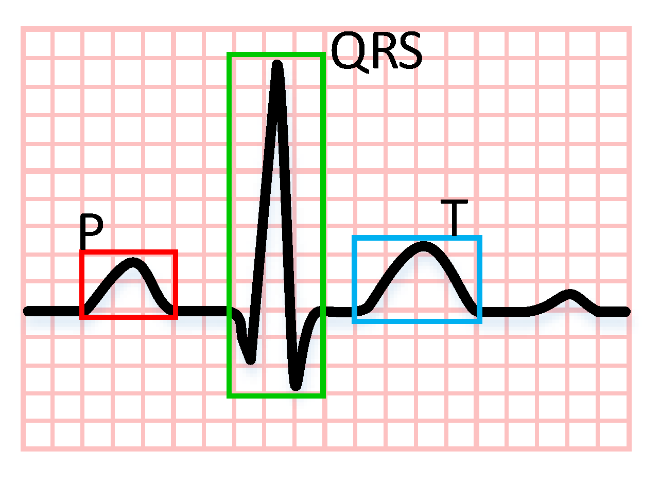
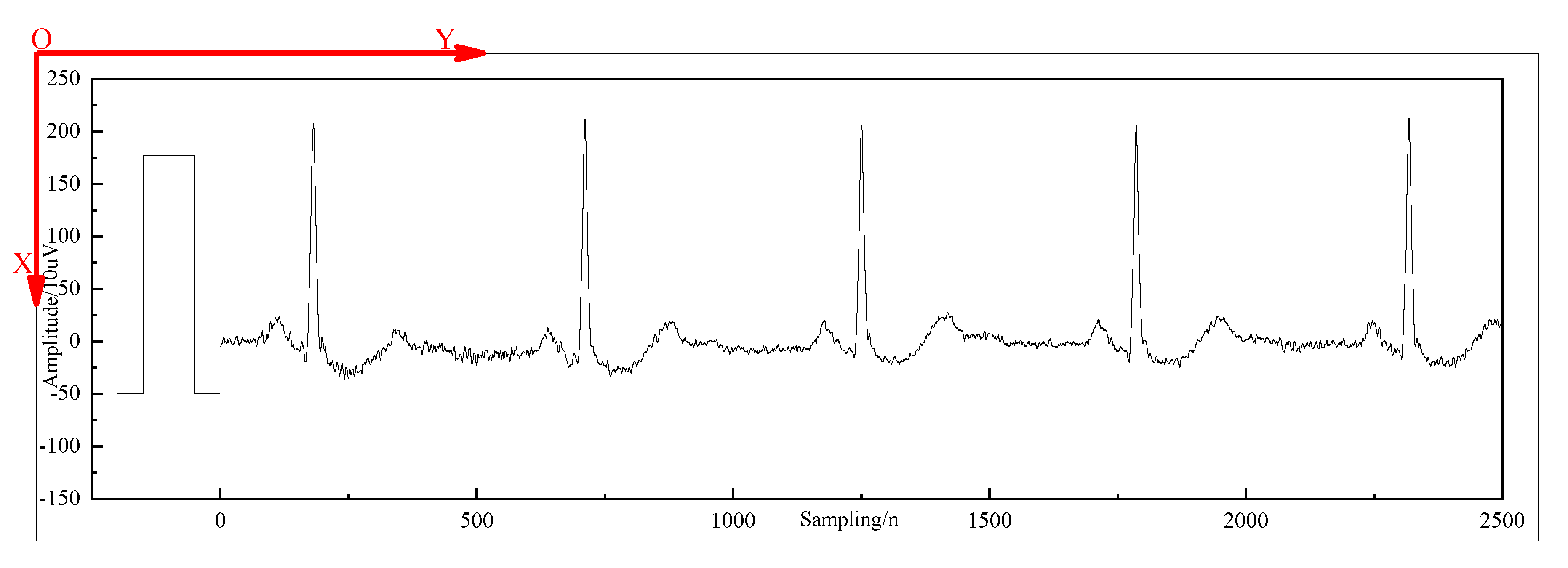
2.1. Research Object

A new disease diagnosis method based on a two-dimensional ECG signal model is proposed in this paper. The main purpose is as shown in Figure 1, which can realize the fine recognition of each refined waveform according to the clinical ECG signal, including a P wave, QRS complex, T wave, etc.

For the successful recognition of an ECG signal, it is necessary to convert it into a two-dimensional image and then establish a coordinate system for the ECG image with a calibration curve, as shown in Figure 2. In this section, the upper left corner pixel of the image is selected as the coordinate origin O, the right is the Y axis, and the downward is the X axis. All the coordinate value recognition in the experiment is based on this coordinate system. The acquisition of coordinates provides a data basis for ECG diagnosis.

Then, using the recognition results with the coordinate position, combined with the transformation relationship between the coordinate value and the actual value in the image, the diagnosis results of specific diseases are finally obtained.

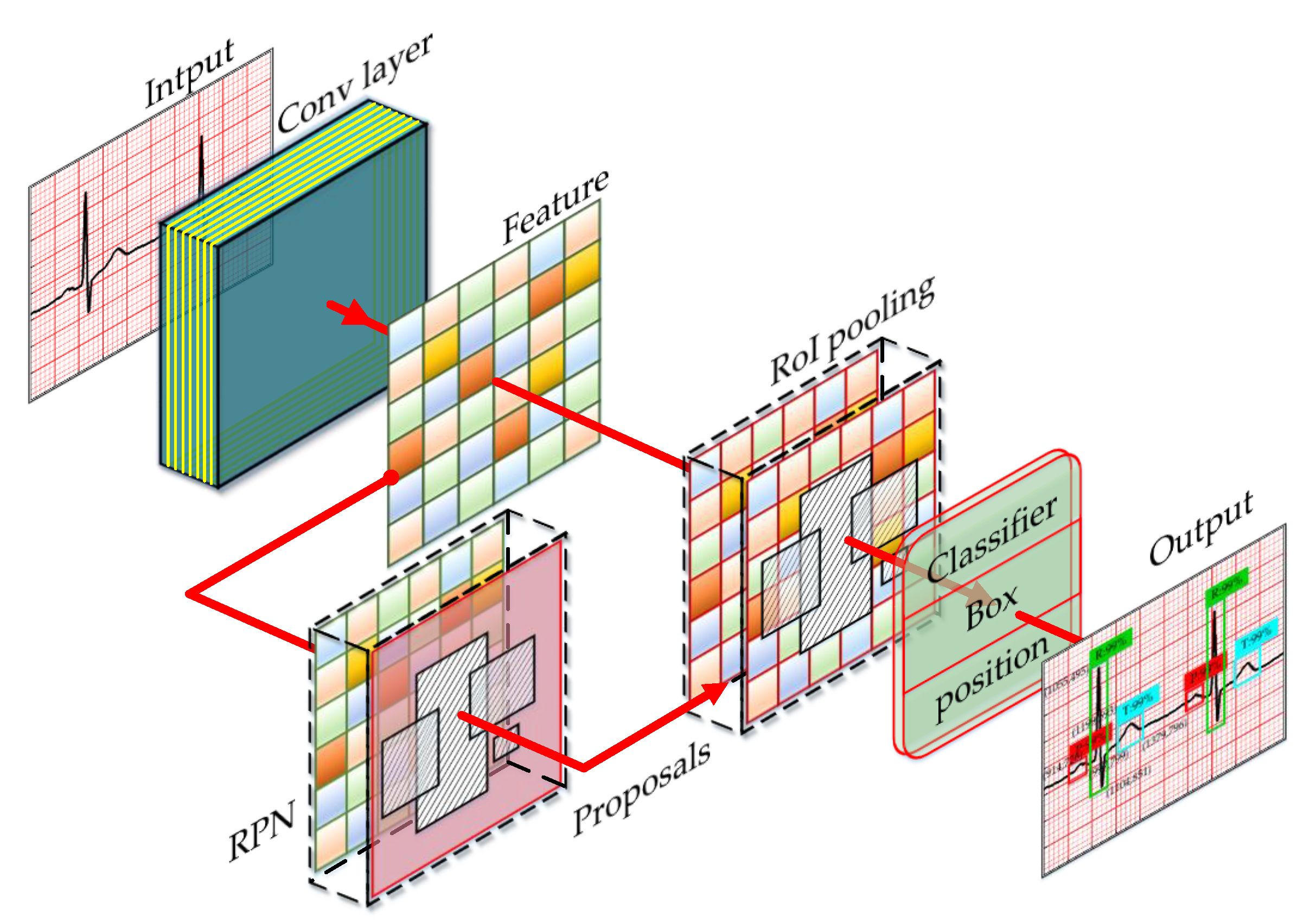
2.2. Diagnosis Model

The algorithm can recognize the target information reflected in the input ECG image quickly and accurately. The system structure is divided into a continuous convolution group layer for feature extraction, a region proposal network (RPN) for optimizing candidate suggestions, a region of interest pooling for comprehensive features, a candidate target, and a classification output. The overall framework of the system based on the refined recognition and diagnosis model is shown in Figure 3.

The feature image results obtained by the continuous convolution layer will be further processed in two channels with different functions. One of the functions is that the feature image results can be directly processed in the regions of interest (RoI) pooling layer. Another function is that the result of the feature image is processed by an RPN module to get a region suggestion and suggestion box output, which will also enter into the RoI pooling layer finally. Therefore, the RoI pooling layer needs to comprehensively refer to the input information of the two channels, and then by using the subsequent full connection layer and after a series of operations such as classifier, region box, and position mark, the final diagnosis output of classification and recognition can be obtained [24].

The advantages of the deep learning diagnosis method are as follows: the system has a two-stage diagnosis structure, which can integrate the multi-target recognition and classification in the image with the target position prediction mechanism. Therefore, it can fully display the details of the analysis results, and it has a better visualization effect.

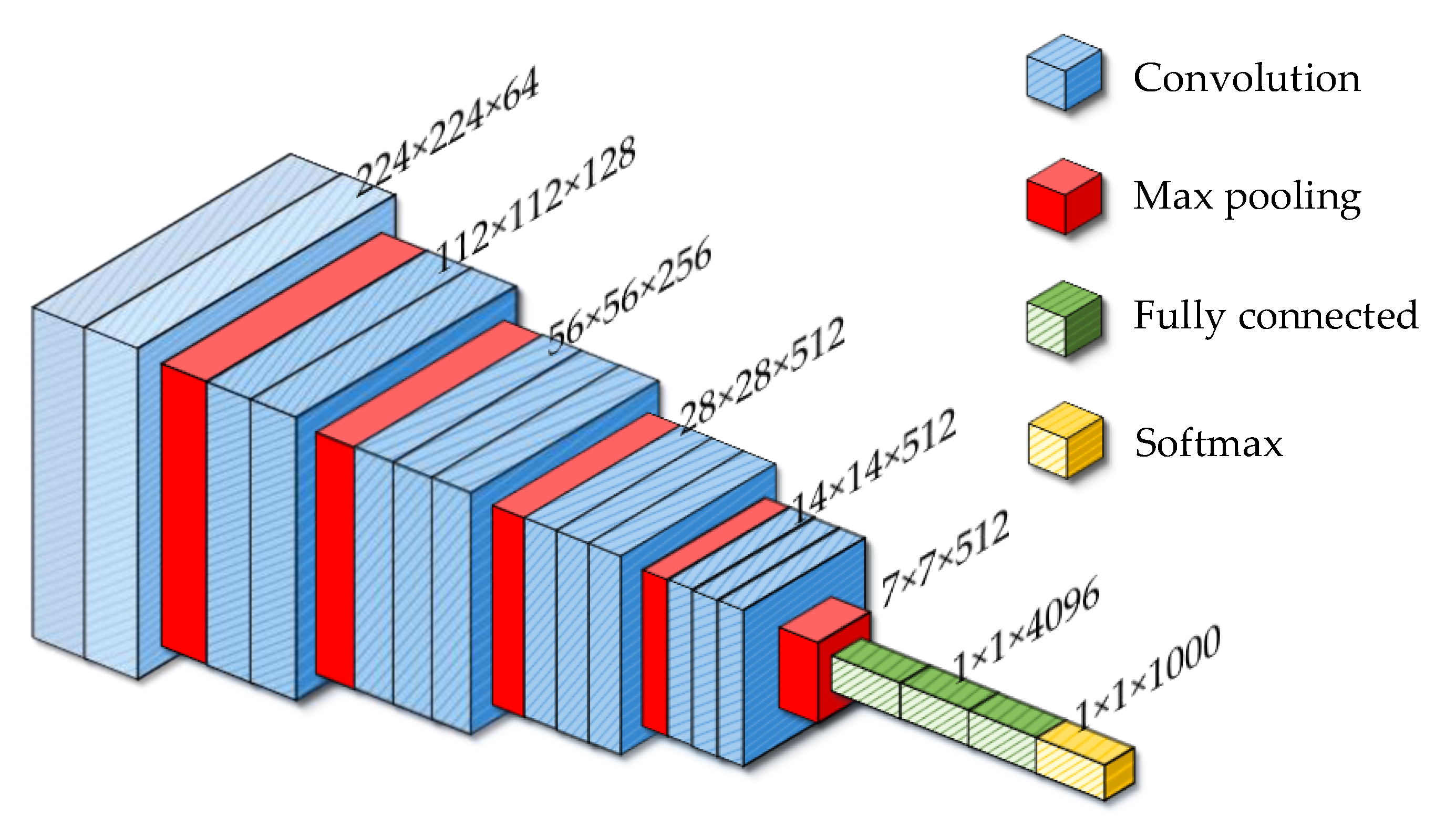
2.2.1. Convolution Neural Network

The continuous convolution layer group structure in the system framework used in Figure 3 sets the VGG16-NET [25] model shown in Figure 4 to generate the feature map. The inner structure of the model includes a convolutional layer, pooling layer, and fully connected layer, among which the number of each layer is 13, 5 and 3. The convolution layer and full connected layer each have weight coefficient attributes and reach 16 layers, which forms the definition standard of the convolution model. The convolution layer and pooling layer are arranged at intervals, and the pooling layer is placed after two or three convolution layer groups, followed by the fully connected layer and finally output through the classification layer. The structures are divided into five levels, among which the sizes of the convolution kernel and pooling kernel to be calculated are 3 × 3 and 2 × 2 respectively. In this way, the calculated results of each layer keep a clear structure. In the calculation process of the VGG16-NET model, the channel number of the input image is doubled from 64 to 512 progressively layer by layer, and the image size is halved from 224 to 7 progressively layer by layer. This rule is that the spatial resolution of the feature map decreases monotonously while the number of channels increases monotonously, which forms the transition between the input ECG image dimension and the classification result vector. The convolution model is used for feature extraction of the information reflected in the original ECG image. Relying on the smaller kernel size and network layer depth, the recognition accuracy of the refined waveform in the ECG conduction cycle can be effectively improved.

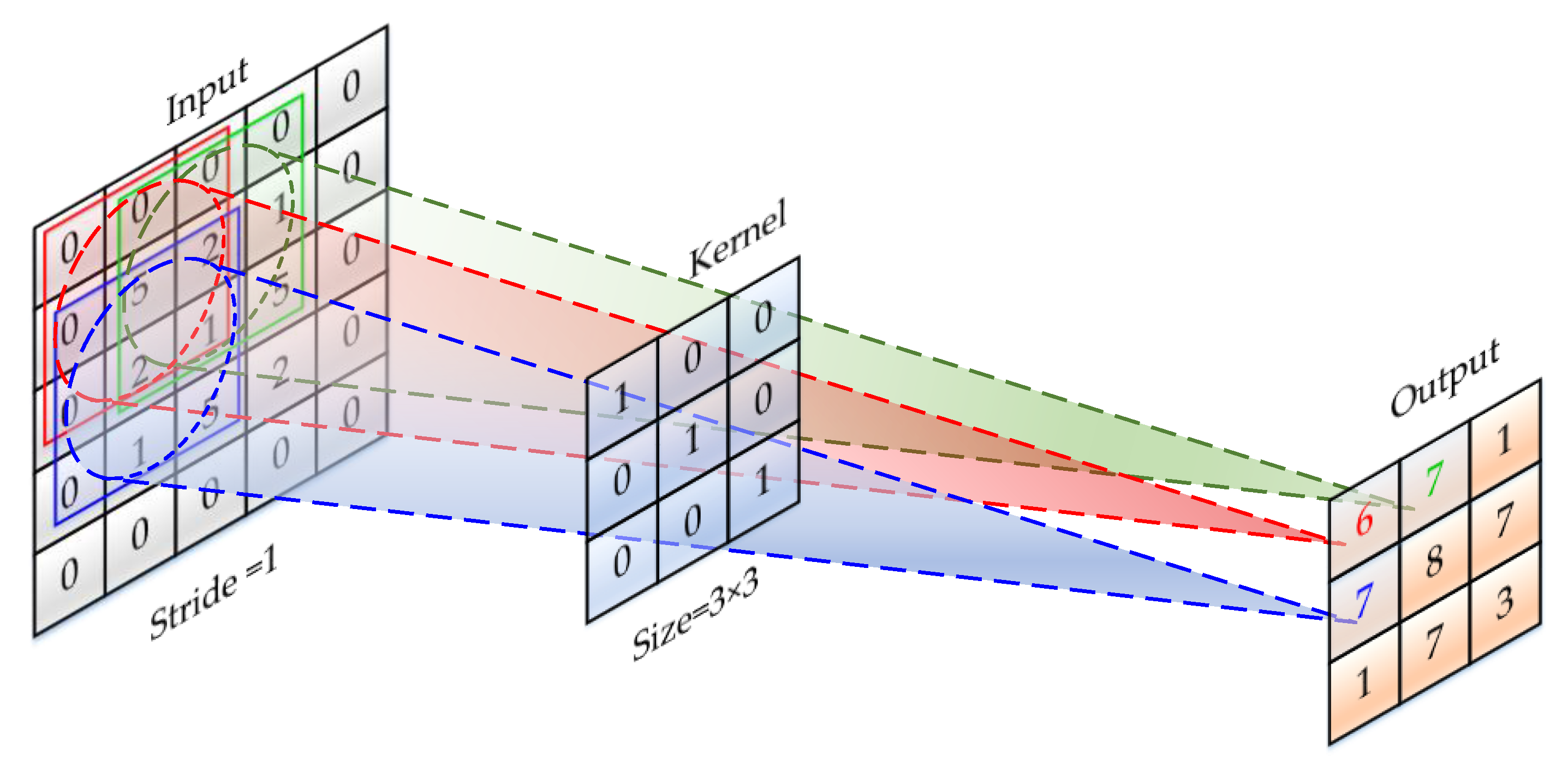
2.2.2. Convolution Layer

The automatic feature extraction of input data is realized by convolution operation. Firstly, convolution operation is performed on two two-dimensional discrete real functions f and g (see Equation (1)) in accordance with Equation (2).

$$\{\begin{array}{lll}f(x,y),\hfill & x=0,1,2,\cdots ,A-1;\hfill & y=0,1,2,\cdots ,B-1\hfill \\ g(x,y),\hfill & x=0,1,2,\cdots ,C-1;\hfill & y=0,1,2,\cdots ,D-1\hfill \end{array}$$

(1)

$$\begin{array}{l}f(x,y)\times g(x,y)\\ ={\displaystyle \sum _{m=0}^{M-1}{\displaystyle \sum _{n=0}^{N-1}f}}(m,n)\cdot g(m-x,n-y)\hspace{1em}\hspace{1em}(x=0,1,2,\cdots M-1;y=0,1,2,\cdots N-1)\end{array}$$

(2)

Based on the above operation rules, the input signal is scanned with a convolution kernel of preset size and a convolution step size [26]; that is, the convolution kernel is used to cover an input signal region of the same size to perform the operation from the input to the corresponding position of the convolution kernel in the region, and the result is taken as a basic element of the convolution output. During the calculation of the convolutional layer, the size of the output image needs to be designed in each layer. The size of an input image is W_i × H_i, the kernel size is K × K, the moving step size is S, and the edge filling pixel is P; the output size W_o and H_o are shown in Equation (3).

$$\begin{array}{l}{W}_o=\frac{W_i-K+2P}{S}+1\\ H_o=\frac{H_i-K+2P}{S}+1\end{array}$$

(3)

For example, if the input matrix size to be convoluted is 5 × 5 and the convolution kernel size is 3 × 3, the outputs of this layer can be obtained when the number of moving steps is 1 and the edge filling pixel is 0, as shown in Figure 5. The process of the convolution calculation is described in detail.

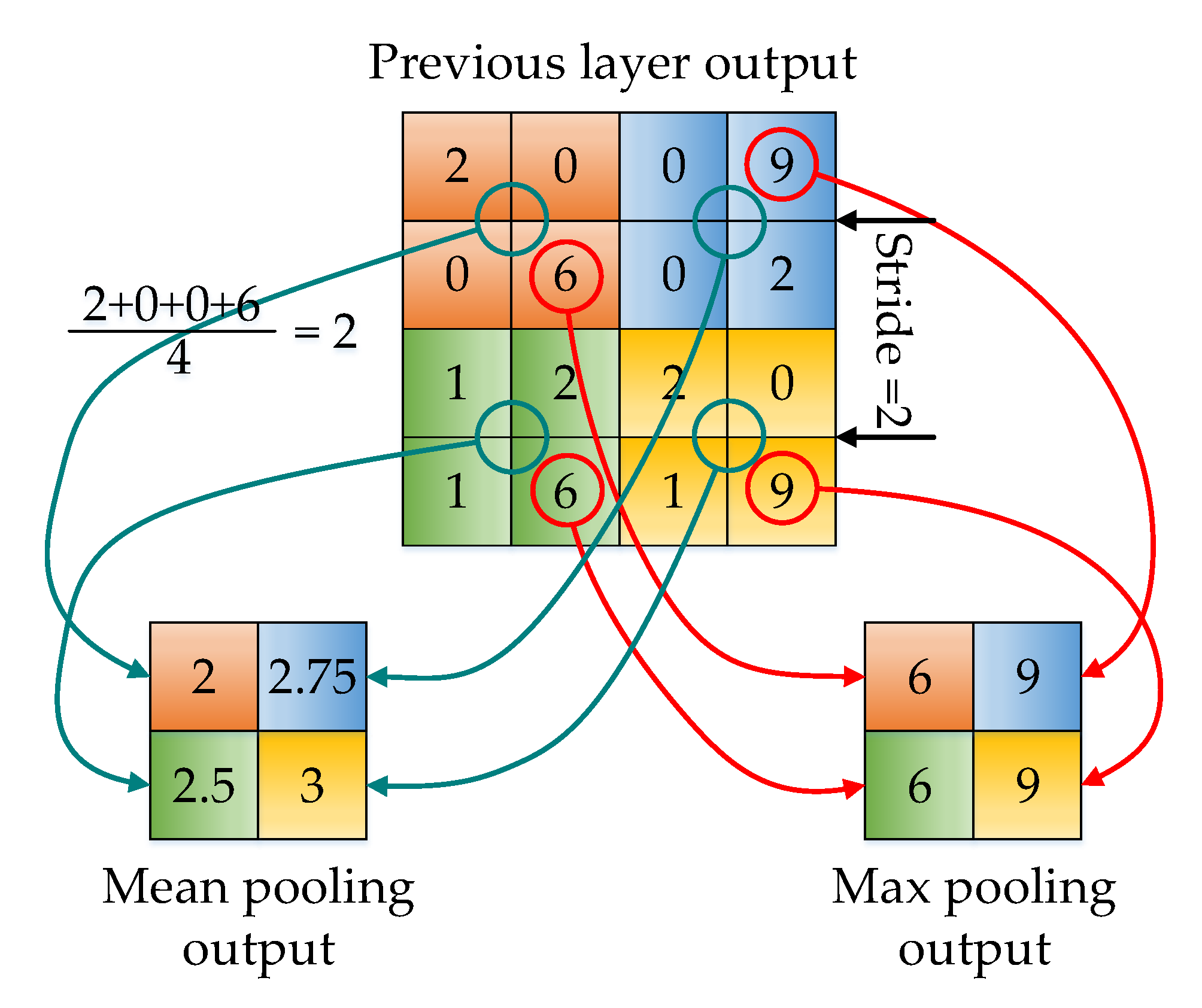
2.2.3. Pooling Layer

In the continuous convolution layer group structure, pooling layers are placed to select or filter data. The compression of the input image is realized, and the dimension reduction effect is achieved. In the pooling method, the maximum pooling and average pooling utilization are higher. The value of P in Equation (3) is usually set to zero. For example, as shown in Figure 6, for 4 × 4 data signals, the window size is set to 2 × 2, and the moving steps are limited to 2. The mean or max pooling method is adopted; that is, the mean value or maximum value is selected from each window as the pooling calculation result [27].

2.2.4. Full Connection Layer

After convolution and pooling calculation, a full connection layer is connected in sequence. Each neural node in this layer is connected with all the neural nodes in the previous layer to form a fully connected network, which is used to synthesize the extracted features. For the processing of two-dimensional information, it is usually converted into one-dimensional vector output and used as the input of the classification step.

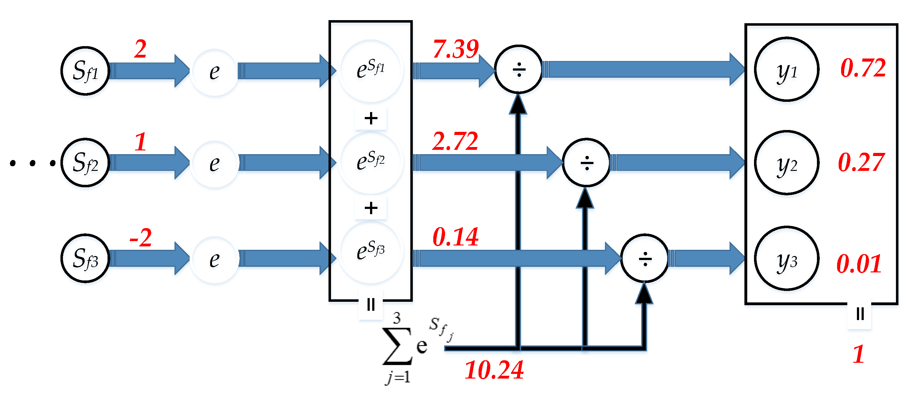
2.2.5. Softmax Layer

In the deep learning network structure, the target classification performance determines the recognition effect of the algorithm. As the output layer of the last level, the Softmax function is widely used to realize multi-classification and output results. Considering the parameters of data dimension X_i and weight W_i in the network, a score function as shown in Equation (4) is defined. Due to the linear characteristics of the function, the ability to distinguish the difference of scoring results is limited.

$$S_f^{\prime }={\displaystyle {\sum }_{i=0}^m{w}_i^{}{x}_i^{}}$$

(4)

In order to increase the difference of scores between different categories and enhance the classification effect, Equation (5) is used to optimize Equation (4). Among them, the score function with e as the base ensures monotonicity, and the score difference is more significant.

$$S_f{=\mathrm{e}}^{{\displaystyle {\sum }_{i=0}^m{w}_i^{}{\mathrm{x}}_i^{}}}$$

(5)

Then, the output of neurons in the previous layer is mapped to a fixed interval (0–1) by using the n-classification normalized probability function Np (see Equation (6)).

$$Np=\left[\begin{array}{c}{\mathrm{y}}_1^{}\\ {\mathrm{y}}_2^{}\\ ⋮\\ {\mathrm{y}}_n^{}\end{array}\right]=\frac{1}{{\displaystyle \sum _{j=1}^n{\mathrm{e}}_j^{{\displaystyle \sum _{i=0}^m{w}_i}{x}_i}}}\left[\begin{array}{c}{\mathrm{e}}_1^{{\displaystyle \sum _{i=0}^m{w}_i}{x}_i}\\ {\mathrm{e}}_2^{{\displaystyle \sum _{i=0}^m{w}_i}{x}_i}\\ ⋮\\ {\mathrm{e}}_n^{{\displaystyle \sum _{i=0}^m{w}_i}{x}_i}\end{array}\right]$$

(6)

where n is the classification category, y_i is the classification output score, and the total score of all multi classification outputs is 1 (see Equation (7)).

$${\displaystyle {\sum }_{i=1}^n{\mathrm{y}}_i^{}=1}$$

(7)

The above process realizes the multi-classification function of the algorithm. In order to illustrate the calculation process of the classification algorithm, Equation (6) is verified by taking three classification outputs as an example, and the process is shown in Figure 7. Let the input S_f1~S_f3 of the three channels be the output of the front layer network. $e^{s_{f1}}$~$e^{s_{f3}}$ is obtained by exponential operation with e as the base, and the three results are accumulated to obtain ${\displaystyle \sum {}_{j=i}^3{e}^{s_{f_j}}}$. The output y₁~y₃ is obtained by dividing $e^{s_f}$ by ${\displaystyle \sum {}_{j=i}^3{e}^{s_{f_j}}}$ respectively. From the result analysis of y, the output results of different categories are different, and they conform to the conclusion of ${\displaystyle {\sum }_{i=1}^3{\mathrm{y}}_i^{}=1}$ [28].

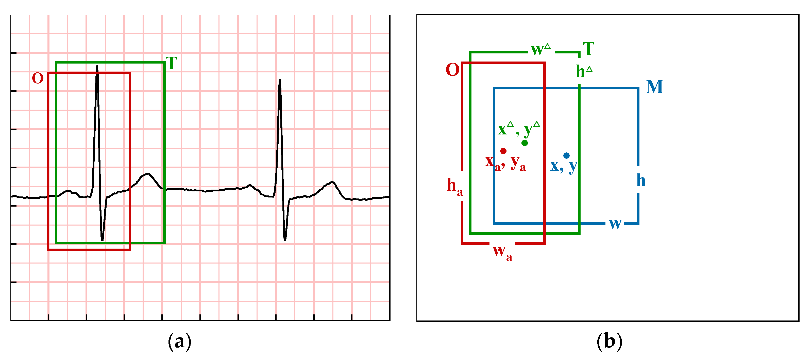
2.3. Region Proposal Network

The RPN network also contains a full convolution layer, which can train the target recognition plan in an end-to-end manner and finally output the boundary and score of the target. After continuous convolution layers, the original image is processed and output in the form of a feature image; then, it is sent to the RPN network as shown in Figure 8. The specific process of feature image calculation in the RPN network is as follows: use a 3 × 3 small-size convolution kernel to move the window on the feature map; then, map it into a low-dimensional vector, and finally, send it to two fully connected layers to get the and regression (REG) layer and classification (CLS) layer. The above output results will eventually be sent to the RoI pooling layer. Usually, in the process of image target region recognition, there will be a deviation between the proposal region and the actual region. The method of box regression can be used to constantly correct the region box to achieve the approximation of the proposal region to the actual region. A large number of anchors will be generated during the correction process, and the values that do not meet the requirements are filtered out by threshold method, and the reserved values are output as proposal parameters.

Take ECG as an example to analyze the boundary box regression principle. In Figure 9a, the green box T represents the actual waveform range in a cardiac conduction cycle, and the red box O represents the initial recognition range of the algorithm for the waveform. Obviously, there is a large deviation between the two boxes, which leads to inaccurate recognition results. In order to reduce the error between the actual value and the recognition value, linear transformation such as translation or zooming is used when the two boxes are close to each other. In this case, it is necessary to set a blue box M as the intermediate variable in Figure 9b. Its function is to make box O equal to box M after linear transformation adjustment and make it close to the actual value box T, so as to accurately recognize the actual range of waveform [29].

From the RPN structure in Figure 8, it is concluded that the anchor is not a single form. In the multi-anchor structure, the normalized total loss is defined as N^Δ, which includes two elements: normalized classification loss NCLS and normalized regression loss NREG; see Equation (8):

$$N^{\Delta }\left(\left\{p_i\right\},\left\{t_i\right\}\right)=\left[\begin{array}{l}\mathrm{NCLS}\left(\left\{p_i\right\},\left\{t_i\right\}\right)=\frac{1}{N_{\mathrm{cls}}}{\displaystyle \sum _i{L}_{\mathrm{cls}}}\left(p_i,p_i^{\Delta }\right)\\ \mathrm{NREG}\left(\left\{p_i\right\},\left\{t_i\right\}\right)=\frac{1}{N_{\mathrm{reg}}}{\displaystyle \sum _i{p}_i^{\Delta }}{L}_{\mathrm{reg}}\left(t_i,t_i^{\Delta }\right)\end{array}\right].$$

(8)

Then, the global loss function L is obtained, as shown in Equation (9):

$$\begin{array}{l}L\left(\left\{p_i\right\},\left\{t_i\right\}\right)\\ =N(1)+\lambda \cdot N(2)\\ =\frac{1}{N_{\mathrm{cls}}}{\displaystyle \sum _i{L}_{\mathrm{cls}}}\left(p_i,p_i^{\Delta }\right)+\lambda \frac{1}{N_{\mathrm{reg}}}{\displaystyle \sum _i{p}_i^{\Delta }}{L}_{\mathrm{reg}}\left(t_i,t_i^{\Delta }\right)\end{array}$$

(9)

The effect of parameter λ is weighted to optimize the balance among the elements of normalized total loss N^Δ. Generally, the optimization status can be obtained by selecting its default value.

3. Verification Experiment

3.1. Dataset of Refined Recognition

The dataset is from the clinical ECG data of 500 different patients in the same provincial hospital. In order to ensure the mutual independence of the data, each data corresponds to a patient; and to display the small details of the classification output results more clearly, each person’s ECG data acquisition time includes 5000 machine sampling points, of which 2500 consecutive sampling points are selected in the experiment, and the segmented data are converted into image format. Since the dataset selected in the experiment needs to be newly built and newly established, a lot of necessary original calibration work is carried out. Based on the above considerations, only 500 samples are selected.

Due to the characteristics of the ECG signal, it is easy for it be interfered by various noises, which has a negative impact on the accuracy of the diagnosis. The sources of noise mainly include power-line interference, resting state, electromyogram (EMG), electrified equipment, and so on. In this experiment, the noise factors were considered in the acquisition of the ECG dataset. Under the premise of the patients’ relative resting state and the correct operation of signal acquisition personnel, the default de-noising settings of the ECG instrument are used to filter noise, such as a low-pass filter at 40 Hz, power frequency filter at 50 Hz, and EMG inhibition at 35 Hz. The purpose of the filter is the ECG data in image format, which is a kind of simulation way for human eyes to observe the ECG report, and it is a direct mapping of the ECG report. These de-noising data can be directly used to output and print the ECG report, and they can be directly used for clinical diagnosis. Therefore, the necessary default de-noising makes the waveform of the ECG signal in the image format consistent with the waveform of an actual clinical ECG report.

Signal acquisition parameters are required as follows: Firstly, the premise of ECG signal acquisition is that the calibration curve parameters of the ECG instrument can be set as 10 mm/1 mV, 2.5 Hz, and the signal sampling frequency is 500 Hz. ECG signals must be printed out after calibration, so the actual output of the calibration curve is very important in two-dimensional image recognition. All output waveforms are realized in proportion to the calibration curve. Secondly, the data selected in the experiment are from the lead II channel and have the characteristics of sinus rhythm, so it is convenient to recognize the waveform of each cardiac conduction cycle in clinical data. Then, the clinical one-dimensional sequence was transformed into a two-dimensional image format. The experimental design includes four types of recognition targets: calibration curve, P, QRS, and T wave.

The experimental design adopts general steps, including training, verification, and testing. Each process needs to select a data volume that meets the verification standard. The data are arranged in sequence, and the samples are selected from the 500 total samples, and assigned to each set. The first 400 samples are selected as a training set and verification set, of which 80% (320 samples) are used as the training set, 20% (80 samples) are used as the verification set, and the last 100 samples are used as the test set.

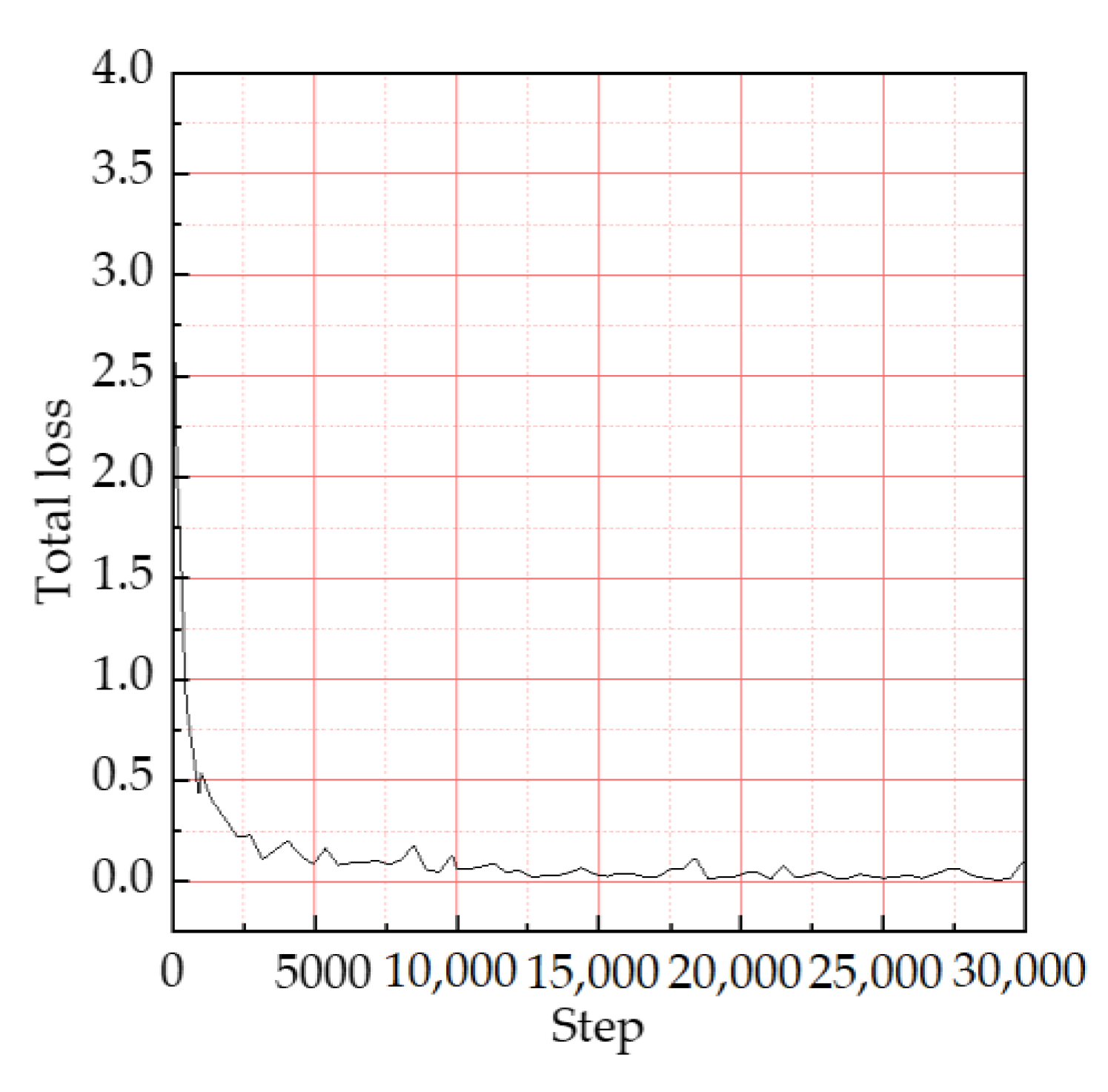
3.2. Training Results

The 2D-ECG image data are trained based on Faster R-CNN to determine the diagnostic model of heart disease. The total loss function curve of clinical data as shown in Figure 10 is obtained through training. The change trend of the curve in the figure is as follows: with the process of the program running, the curve decreases rapidly from the initial state value of 3.54 in the longitudinal direction, fluctuates slightly when the value approaches 0 when reaching 10,000 steps, and maintains stable curve fluctuation when reaching 30,000 steps. Therefore, it is feasible to apply the model to the identification of clinical data.

Many research studies only recognize part of the ECG waveform, and this method can recognize multiple parameter details at the same time. The refined recognition results of this algorithm for two-dimensional ECG signals include four kinds of tags: O, P, R, and T, which represent the calibration curve, P wave, QRS complex, and T wave, respectively. The recognition results are shown in Figure 11. The scope of each type of refined waveform is clearly marked in the figure. Meanwhile, the coordinate values of the upper left and lower right of the recognition box are marked for the recognized region. These values can be used for subsequent calculation, such as the height and duration of the waveform, which can be used as the basis for ECG diagnosis.

Faster R-CNN is used to recognize the waveforms of clinical experimental data samples. The recognition results of refined ECG parameters are shown in

Table 1. Recognition accuracy of refined ECG parameters.

Category	Description	Accuracy
O	calibration curve	0.9968
P	P wave	0.9832
R	QRS complex	0.9885
T	T wave	0.9890
Average accuracy	-	0.9894

.

The recognition accuracy of the waveform labeled as Category O is 99.68%, that of Category P is 98.32%, that of Category R is 98.85%, and that of Category T is 98.90%. The experimental results verify that the proposed method has an overall average accuracy of 98.94%. Therefore, the proposed method is feasible for medical auxiliary diagnosis. The research results are compared with others in the literature (see

Table 2. Comparison with other literatures.

Recognition Method	Average Accuracy (%)	Waveform Type	Waveform Number
Faster R-CNN	98.94	O, P, QRS, T	4
LSTM [30]	92.00	P, QRS, T	3
4-LSTM [31]	98.48	P	1
CNN + ELM [32]	98.77	QRS	1
SVM [33]	95.26	QRS	1

) to fully reflect the effectiveness of the model proposed in this section. Firstly, the selected comparative literature is based on one-dimensional sequence, and the waveform in the cardiac conduction cycle is taken as the recognition object. Among them, literature [30] used the method of the long short-term memory (LSTM) model to recognize three types of refined waveforms, and the average accuracy of 92.00 was obtained. The method of multi-LSTM model fusion was designed in literature [31], which only recognized a single P wave and achieved an average accuracy of 98.48. Literature [32], a method combining a CNN and ELM model, was used to recognize only a single QRS complex, with an average accuracy of 98.77. In literature [33], an support vector machine (SVM) model was used to recognize a single QRS complex, with an average accuracy of 95.26.

Through analysis and comparison, it is found that adopting a two-dimensional ECG signals algorithm based on Faster R-CNN for identification and diagnosis can achieve higher recognition accuracy, recognize more kinds of refined waveforms, and have more intuitive visual results.

4. Analysis and Diagnosis

It is of practical significance to diagnose the main parameters of ECG signals by the coordinate parameter values of each refined waveform in the cardiac conduction cycle. Firstly, it is necessary to establish the mapping relationship between the time and amplitude parameters of ECG signals and the coordinate parameters in the picture. The clinical ECG data used in this section are when the calibration curve parameter of the ECG instrument is set as 10 mm/1mV, 2.5 Hz, and 0.2 s during the high level. It is concluded that the height of the calibration curve takes up two big grids, and the minimum cell of amplitude along the longitudinal axis is 1 mm/0.1 mV. The paper speed of ECG is set at 25 mm/s, the signal sampling frequency is 500 Hz, and the sampling cycle time is 0.002 s; then, the corresponding time length of 20 samplings is 0.04 s, and the time span occupies a minimum cell; in this way, the time length of 100 samplings is 0.2 s, which occupies one big grid. In the ECG report, the horizontal axis time length corresponding to a minimum cell is 0.04 s; a large grid contains five minimum cells, and the duration is 0.2 s; therefore, the duration of five large grids is 1 s, as shown in

Table 3. Time and amplitude standard of gridding in ECG report.

Parameters	Time (Width) s/Amplitude (Height) mm
1 cell width	0.04 s
1 big grid width	0.2 s
5 big grid width	1 s
Duration width of sampling period	0.002 s
Calibration curve high level width	0.2 s
Calibration curve height with 2 grids	10 mm

.

Therefore, the width and height of the calibration curve as the identification standard are known. Therefore, based on the method of mapping the time and amplitude of ECG signals to the coordinates in the picture, it is of practical significance to recognize and diagnose the parameters of each refined waveform of ECG signals [34,35]. Therefore, establishing the position relation between coordinates and realizing the mapping between the real signal value and the image coordinates are the necessary steps for the algorithm model to realize the diagnosis of heart disease. First of all, the coordinate equations need to be established. For each marked recognition box, the coordinates of the top left and bottom right points are marked with an array B containing four elements, as shown in Equation (10):

$$B={[X_{N_1},Y_{N_1},X_{N_2},Y_{N_2}]}_{}{,}_{} N\in (O{,}_{} P{,}_{} QRS{,}_{} T_{}\cdots )$$

(10)

where N is the refined waveform parameter to be recognized, $(X_{N_1},Y_{N_1})$ is the upper left corner coordinate point, and $(X_{N_2},Y_{N_2})$ is the bottom right-hand corner coordinate point. Secondly, the mapping relationship between actual time interval t_N, amplitude height h_N, and image coordinate value is established, as shown in Equation (11).

$$\{\begin{array}{l}{t}_N=t_u\cdot \left(X_{N_2}-X_{N_1}\right)\hfill \\ h_N=h_u\cdot \left(Y_{N_2}-Y_{N_1}\right)\hfill \end{array}$$

(11)

where t_u is the unit pixel experience time and h_u is the unit pixel amplitude height. In this section, the calibration curve parameter values can be known from

Table 4. Calculation results of time and amplitude of the main parameters in ECG.

Parameter N	Calculation by Formula
	tN (s)	hN (mm)
O	0.2	10
P	0.114	1.11
QRS	0.068	5.410
T	0.229	3.040
P-P	0.846	-
P–R interval	0.194	-
P–R segment	0.08	-
S–T segment	0.131	-
S–T interval	0.379	-
Q–T interval	0.447	-

, so Equation (12) is available,

$$t_u=\frac{0.2}{X_{O_2}-X_{O_1}}(s); h_u=\frac{10}{Y_{O_2}-Y_{O_1}}\left(mm\right)$$

(12)

The mapping between the real value of the cardiac electrophysiological signal and image coordinates is realized by substituting the unit parameters t_u and h_u into Equation (11). Thus, the fine range recognition of ECG waveform can be calculated by the above formula. Taking Figure 11a as an example, the calculation results of the main parameters in ECG are shown in Table 4. After analysis, it is found that although only four types of waveforms are identified in the experiment, the analysis of the important parameters of other ECG signals can be obtained by the coordinate relationship of the above four types of parameters.

The applicability of the model proposed in this paper is further verified by combining the diagnosis and analysis of different clinical diseases [36,37]. According to the characteristics of the existing samples, using the waveform parameters identified by the algorithm model proposed in this paper, some clinical examples of disease diagnosis are shown in

Table 5. Application analysis of the proposed diagnosis model.

Type of N	Diagnostic Basis	Possible Disease Category
P	Calculate P shape, width, height, etc.	Atrial hypertrophy, hyperkalemia, etc.
Q	The calculated Q width is out of the normal range.	Myocardial infarction, myocarditis, etc.
QRS	Amplitude increase/decrease Width increased.	Myocardial hypertrophy/electrolyte disorder, etc. Bundle branch block, myocardial drugs, etc.
S-T	Morphological changes, elevation or depression, lengthening and shortening, etc.	Myocardial ischemia, etc.
T	Morphological changes, such as towering, low flat, inverted, etc.	Hyperkalemia, etc.
U	The U-wave enlarged obviously.	Hypokalemia, etc.
Q–T	Span extension.	Myocardial ischemia, drugs, etc.
P, R, P–R, P–P, QRS	The calculated P-R value was greater than 0.21s and increased continuously.	I-atrioventricular block, etc.
	Periodic calculation of P-R prolongation, continuous recognition of conduction cycle waveform, until a QRS missing after P.	II-1 atrioventricular block, etc.
	P–R was constant and QRS missing was proportional to P.	II-2 atrioventricular block, etc.
	The adjacent P is equidistant and R is equidistant. P is not related to R.	III-atrioventricular block, etc.

.

5. Discussion

The proposed diagnosis method based on 2D-ECG and Faster R-CNN has advantages over the traditional one-dimensional sequence method in classification and diagnosis performance. Firstly, it realizes the conversion of a cardiac electrophysiological signal from a one-dimensional time series to a two-dimensional image, which has the ability of describing information from multiple angles; secondly, it can identify and diagnose a complete beat in the cardiac conduction cycle, so as to realize the fine recognition between or within the cardiac beats. Combined with the transformation relationship between the coordinate value recognized in the image and the actual value, the diagnosis of specific diseases can be realized. Compared with different models in four literatures, the results show that the model proposed in this paper improves and innovates in the recognition and diagnosis of cardiac electrophysiological signals, and it has more intuitive visualization results.

Due to the complexity of the cardiac system, this research has some limitations. Firstly, the experimental design only considers the disease diagnosis process based on a single channel standard II lead. Although this lead can reflect the characteristics of the ECG signal and most research studies are based on this lead, a single lead has limitations on the analysis of diverse ECG data. Secondly, 2500 sampling points are selected for each sample duration. The main purpose of this segmentation is to verify the feasibility of the detailed parameter expected identification, but it has limitations for progressive heart disease diagnosis.

6. Conclusions

In this paper, a novel faster region recognition method for 2D-ECG at the image level is established. The ECG data with sinus heart rate are taken as the research object, the refined recognition and diagnosis of each detailed waveform is realized, and the average recognition accuracy reaches 98.94%. The experimental results show that the proposed method is feasible for medical auxiliary diagnosis.

In the future work, there are still many aspects of ECG analysis and diagnosis that need to be further improved and carried out. First of all, the comprehensive diagnosis and analysis of multiple leads in clinical application needs further research. The 12 leads data analysis model is used to improve the accuracy of clinical data identification by the correlation between different leads. Secondly, increasing the sampling time of a single image is used to improve the recognition ability of the detailed parameters within a cardiac beat or between the multi cardiac beats, which is conducive to improving the classification of diseases and the application scope of diagnosis. Finally, the main purpose is to increase the number of samples for different diseases and each disease type.

References

1. Oh, S.L.; Hagiwara, Y.; Raghavendra, U.; Yuvaraj, R.; Arunkumar, N.; Murugappan, M.; Acharya, U.R. A deep learning approach for Parkinson’s disease diagnosis from EEG signals. Neural Comput. Appl. 2020, 32, 10927–10933. [Google Scholar] [CrossRef]
2. Vani, S.; Suresh, G.R.; Balakumaran, T.; Ashawise, C.T. EEG Signal Analysis for Automated Epilepsy Seizure Detection Using Wavelet Transform and Artificial Neural Network. Med. Imaging Health Inform. 2019, 9, 1301–1306. [Google Scholar] [CrossRef]
3. Nasser, I.M.; Abu-Naser, S.S. Lung Cancer Detection Using Artificial Neural Network. Int. J. Eng. Inf. Syst. 2019, 3, 17–23. [Google Scholar]
4. Xia, P.; Hu, J.; Peng, Y. EMG-based estimation of limb movement using deep learning with recurrent convolutional neural networks. Artif. Organs 2018, 42, E67–E77. [Google Scholar] [CrossRef]
5. Rehman, M.Z.U.; Waris, A.; Gilani, S.O.; Jochumsen, M.; Niazi, I.K.; Jamil, M.; Farina, D.; Kamavuako, E.N. Multiday EMG-based classification of hand motions with deep learning techniques. Sensors 2018, 18, 2497. [Google Scholar] [CrossRef] [PubMed] [Green Version]
6. Lakshmanaprabu, S.K.; Mohanty, S.N.; Shankar, K.; Arunkumar, N.; Ramirez, G. Optimal deep learning model for classification of lung cancer on CT images. Future Gener. Comput. Syst. 2019, 92, 374–382. [Google Scholar]
7. Han, Z.; Wei, B.; Zheng, Y.; Yin, Y.; Li, K.; Li, S. Breast cancer multi-classification from histopathological images with structured deep learning model. Sci. Rep. 2017, 7, 1–10. [Google Scholar] [CrossRef]
8. Mustaqeem, A.; Anwar, S.M.; Majid, M. Multiclass classification of cardiac arrhythmia using improved feature selection and SVM invariants. Comput. Math. Methods Med. 2018, 2018, 7310496. [Google Scholar] [CrossRef] [Green Version]
9. Zhang, Y.; Li, J. The dominant T wave cluster and One-Class SVM based analysis of multilead ECG for classification of myocardial infarction. In Proceedings of the Third International Conference on Biological Information and Biomedical Engineering, Hangzhou, China, 20–22 June 2019; pp. 1–7. [Google Scholar]
10. Saadawy, E.I.; Tantawi, M.; Shedeed, H.A.; Tolba, M.F. Electrocardiogram (ECG) classification based on dynamic beats segmentation. In Proceedings of the 10th International Conference on Informatics and Systems, Cairo, Egypt, 6–25 February 2016; pp. 75–80. [Google Scholar]
11. Baloglu, U.B.; Talo, M.; Yıldırım, Ö.; Tan, R.S.; Acharya, U.R. Classification of myocardial infarction with multi-lead ECG signals and deep CNN. Pattern Recognit. Lett. 2019, 122, 23–30. [Google Scholar] [CrossRef]
12. Black, N.; D’Souza, A.; Wang, Y.; Piggins, H.; Dobrzynski, H.; Morris, G.; Boyett, M.R. Circadian rhythm of cardiac electrophysiology, arrhythmogenesis, and the underlying mechanisms. Heart Rhythm 2019, 16, 298–307. [Google Scholar] [CrossRef] [Green Version]
13. Dietrichs, E.S.; McGlynn, K.; Allan, A.; Connolly, A.; Bishop, M.; Burton, F.; Kettlewell, S.; Myles, R.; Tveita, T.; Smith, G.L. Moderate but not severe hypothermia causes pro-arrhythmic changes in cardiac electrophysiology. Cardiovasc. Res. 2020, 116, 2081–2090. [Google Scholar] [CrossRef] [PubMed]
14. Pyakillya, B.; Kazachenko, N.; Mikhailovsky, N. Deep learning for ECG classification. J. Phys. Conf. Ser. IOP Publ. 2017, 913, 012004. [Google Scholar] [CrossRef]
15. Mousavi, S.; Afghah, F. Inter-and intra-patient ecg heartbeat classification for arrhythmia detection: A sequence to sequence deep learning approach. In Proceedings of the ICASSP 2019–2019 IEEE International Conference on Acoustics, Speech and Signal Processing (ICASSP), Brighton, UK, 12–17 May 2019; IEEE: Piscataway, NJ, USA, 2019; pp. 1308–1312. [Google Scholar]
16. Zhang, Q.; Zhou, D.; Zeng, X.; Heart, I.D. A multiresolution convolutional neural network for ECG-based biometric human identification in smart health applications. IEEE Access 2017, 5, 11805–11816. [Google Scholar] [CrossRef]
17. Acharya, U.R.; Fujita, H.; Lih, O.S.; Hagiwara, Y.; Tan, J.H.; Adam, M. Automated detection of arrhythmias using different intervals of tachycardia ECG segments with convolutional neural network. Inf. Sci. 2017, 405, 81–90. [Google Scholar] [CrossRef]
18. Bhurane, A.A.; Sharma, M.; Tan, R.-S.; Acharya, U.R. An efficient detection of congestive heart failure using frequency localized filter banks for the diagnosis with ECG signals. Cogn. Syst. Res. 2019, 55, 82–94. [Google Scholar] [CrossRef]
19. Li, D.; Zhang, H.; Zhang, M. Wavelet de-noising and genetic algorithm-based least squares twin SVM for classification of arrhythmias. Circuits Syst. Signal Process. 2017, 36, 2828–2846. [Google Scholar] [CrossRef]
20. Gliner, V.; Yaniv, Y. An SVM approach for identifying atrial fibrillation. Physiol. Meas. 2018, 39, 094007. [Google Scholar] [CrossRef]
21. Castillo, J.A.; Granados, Y.C.; Ariza, C.A.F. Patient-Specific Detection of Atrial Fibrillation in Segments of ECG Signals using Deep Neural Networks. Ciencia E Ingenieria Neogranadina 2020, 30, 45–58. [Google Scholar] [CrossRef]
22. Labati, R.D.; Muñoz, E.; Piuri, V.; Sassi, R.; Scotti, F. Deep-ECG: Convolutional neural networks for ECG biometric recognition. Pattern Recognition Letters 2019, 126, 78–85. [Google Scholar] [CrossRef]
23. Mahmud, T.; Fattah, S.A.; Saquib, M. DeepArrNet: An Efficient Deep CNN Architecture for Automatic Arrhythmia Detection and Classification from Denoised ECG Beats. IEEE Access 2020, 8, 104788–104800. [Google Scholar] [CrossRef]
24. Ren, S.; He, K.; Girshick, R.; Sun, J. Faster r-cnn: Towards real-time object detection with region proposal networks. In Proceedings of the Advances in Neural Information Processing Systems, Montreal, QC, Canada, 7–10 December 2015; pp. 91–99. [Google Scholar]
25. Simonyan, K.; Zisserman, A. Very Deep Convolutional Networks for Large-Scale Image Recognition. arXiv 2015, arXiv:14091556. [Google Scholar]
26. Avanzato, R.; Beritelli, F. Automatic ECG Diagnosis Using Convolutional Neural Network. Electronics 2020, 9, 951. [Google Scholar] [CrossRef]
27. Guaragnella, C.; Rizzi, M.; Giorgio, A. Marginal Component Analysis of ECG Signals for Beat-to-Beat Detection of Ventricular Late Potentials. Electronics 2019, 8, 1000. [Google Scholar] [CrossRef] [Green Version]
28. Kharshid, A.; Alhichri, H.S.; Ouni, R.; Bazi, Y. Classification of Short-time Single-lead ECG Recordings Using Deep Residual CNN. In Proceedings of the 2019 2nd International Conference on new Trends in Computing Sciences (ICTCS), Amman, Jordan, 9–11 October 2019; IEEE: Piscataway, NJ, USA, 2019; pp. 1–6. [Google Scholar]
29. Luo, C.; Jiang, H.; Li, Q.; Rao, N. Multi-label Classification of Abnormalities in 12-Lead ECG Using 1D CNN and LSTM. In Machine Learning and Medical Engineering for Cardiovascular Health and Intravascular Imaging and Computer Assisted Stenting; Springer: Cham, Switzerland, 2019; pp. 55–63. [Google Scholar]
30. Abrishami, H.; Han, C.; Zhou, X.; Campbell, M.; Czosek, R. Supervised ecg interval segmentation using lstm neural network. In Proceedings of the International Conference on Bioinformatics & Computational Biology (BIOCOMP), Las Vegas, NV, USA, 19–21 March 2018; pp. 71–77. [Google Scholar]
31. Peimankar, A.; Puthusserypady, S. An Ensemble of Deep Recurrent Neural Networks for P-wave Detection in Electrocardiogram. In Proceedings of the ICASSP 2019–2019 IEEE International Conference on Acoustics, Speech and Signal Processing (ICASSP), Brighton, UK, 12–17 May 2019; pp. 1284–1288. [Google Scholar]
32. Zhou, S.; Tan, B. Electrocardiogram soft computing using hybrid deep learning CNN-ELM. Appl. Soft Comput. 2019, 86, 105778. [Google Scholar] [CrossRef]
33. Shdefat, A.; Joo, M.; Kim, H. A Method of Analyzing ECG to Diagnose Heart Abnormality utilizing SVM and DWT. J. Multimed. Inf. Syst. 2016, 3, 35–42. [Google Scholar]
34. Yuen, B.; Dong, X.; Lu, T. Inter-Patient CNN-LSTM for QRS Complex Detection in Noisy ECG Signals. IEEE Access 2019, 7, 169359–169370. [Google Scholar] [CrossRef]
35. Sarvan, Ç.; Özkurt, N. ECG Beat Arrhythmia Classification by using 1-D CNN in case of Class Imbalance. In Proceedings of the 2019 Medical Technologies Congress (TIPTEKNO), Izmir, Turkey, 3–5 October 2019; IEEE: Piscataway, NJ, USA, 2019; pp. 1–4. [Google Scholar]
36. Zhang, K.; Li, X.; Xie, X.; Wang, Q. Research on arrhythmia detection algorithm based on deep learning. Med. Health Equip. 2018, 39, 6–9. [Google Scholar]
37. Zheng, Z.; Chen, Z.; Hu, F.; Zhu, J.; Tang, Q.; Liang, Y.; Zheng, Z.; Chen, Z.; Hu, F.; Zhu, J.; et al. An Automatic Diagnosis of Arrhythmias Using a Combination of CNN and LSTM Technology. Electronics 2020, 9, 121. [Google Scholar] [CrossRef] [Green Version]
Figure 1. Examples of refined recognition to electrocardiogram (ECG) parameters.
Information 11 00556 g001
Figure 2. Establishment rules of a two-dimensional electrocardiogram (ECG) image coordinate system.
Information 11 00556 g002
Figure 3. Overall framework of the refined recognition and diagnosis model.
Information 11 00556 g003
Figure 4. The continuous convolution layer group structure of VGG16.
Information 11 00556 g004
Figure 5. Examples of two-dimensional convolution operation.
Information 11 00556 g005
Figure 6. Example of mean pooling and max pooling operation.
Information 11 00556 g006
Figure 7. Example of operation of normalized probability classification function.
Information 11 00556 g007
Figure 8. Detailed functions of region proposal network.
Information 11 00556 g008
Figure 9. Example of the boundary box regression principle. (a) Recognition with obvious deviation; (b) Deviation adjustment process.
Information 11 00556 g009
Figure 10. Total loss function curve of clinical data obtained by training.
Information 11 00556 g010
Figure 11. Recognition results of ECG waveform. (ae) describe the recognition results of five different samples in the total data.
Information 11 00556 g011aInformation 11 00556 g011b