Convolutional Support Vector Models: Prediction of Coronavirus Disease Using Chest X-rays

 ,
, 
 and
and
Abstract
1. Introduction
2. Convolutional Networks
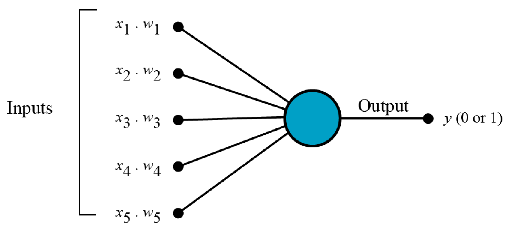
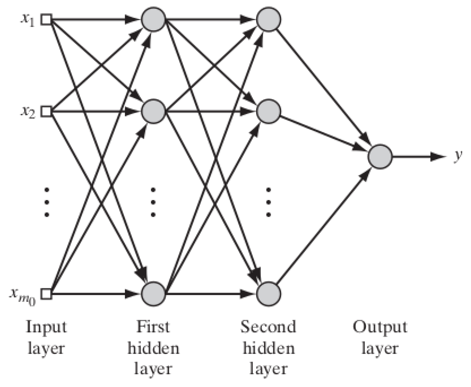
2.1. Multi-Layer Perceptron Neural Networks
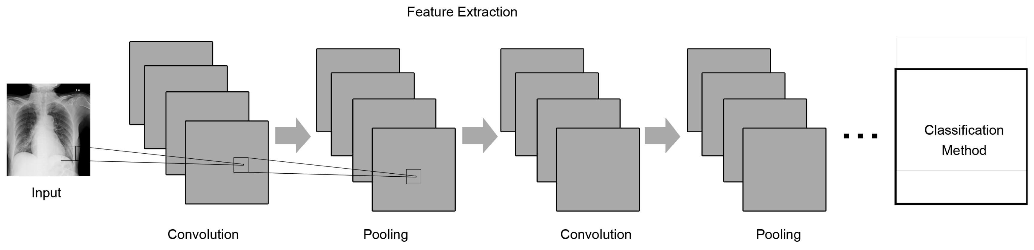
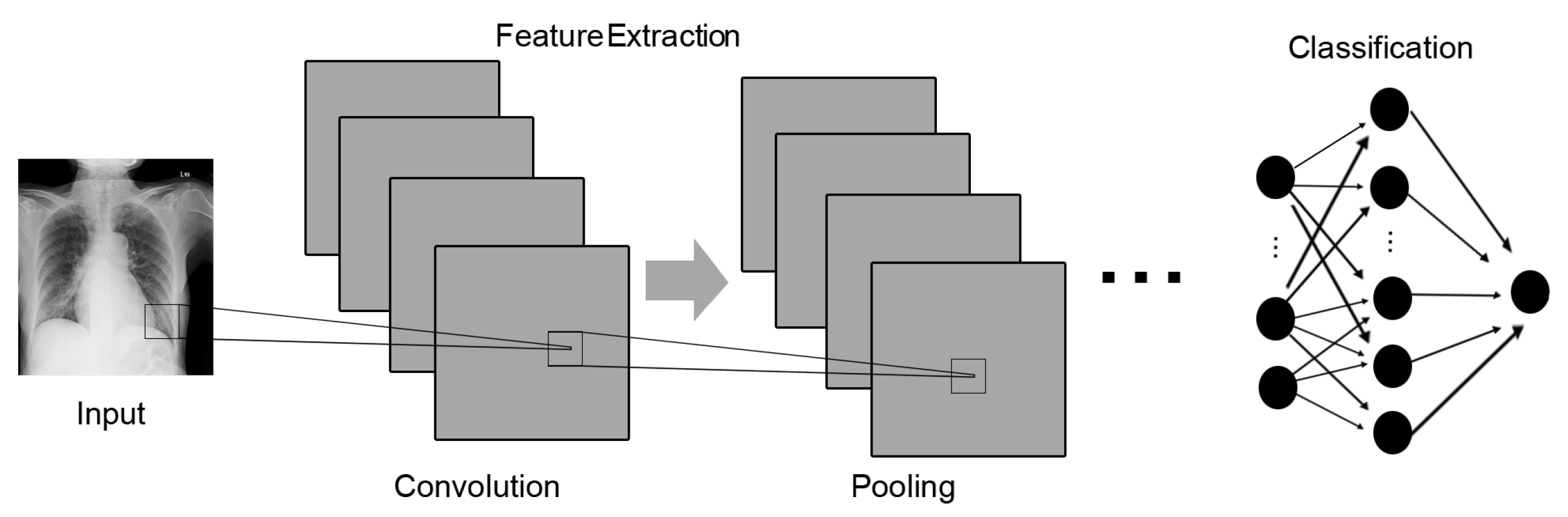
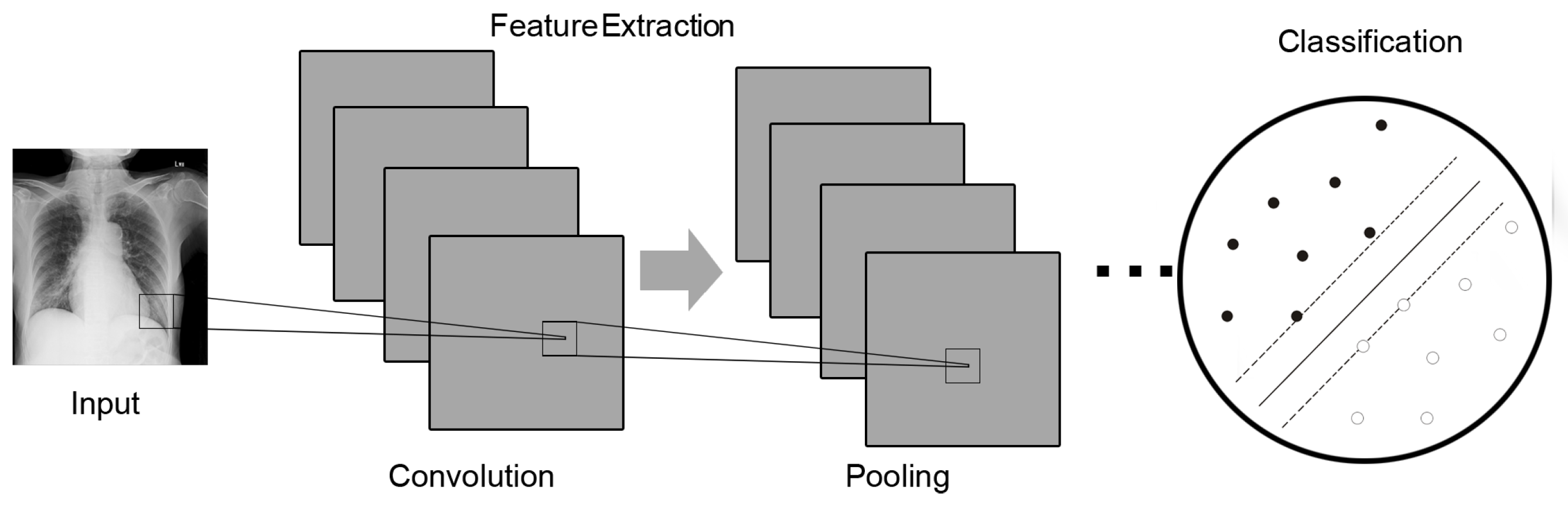
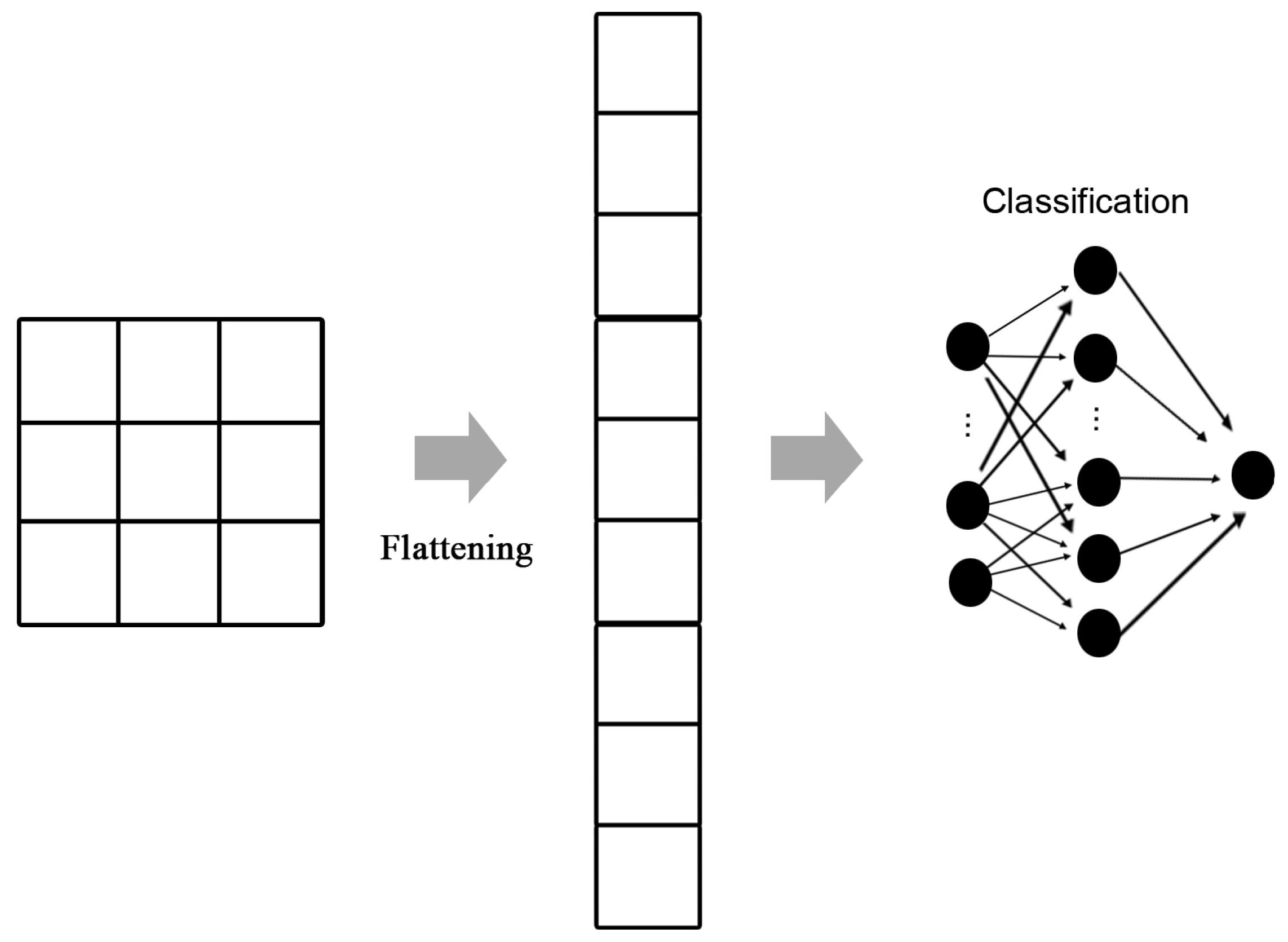
2.2. Convolution Neural Networks
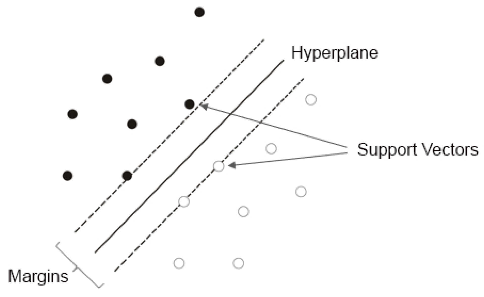
3. Support Vector Machines
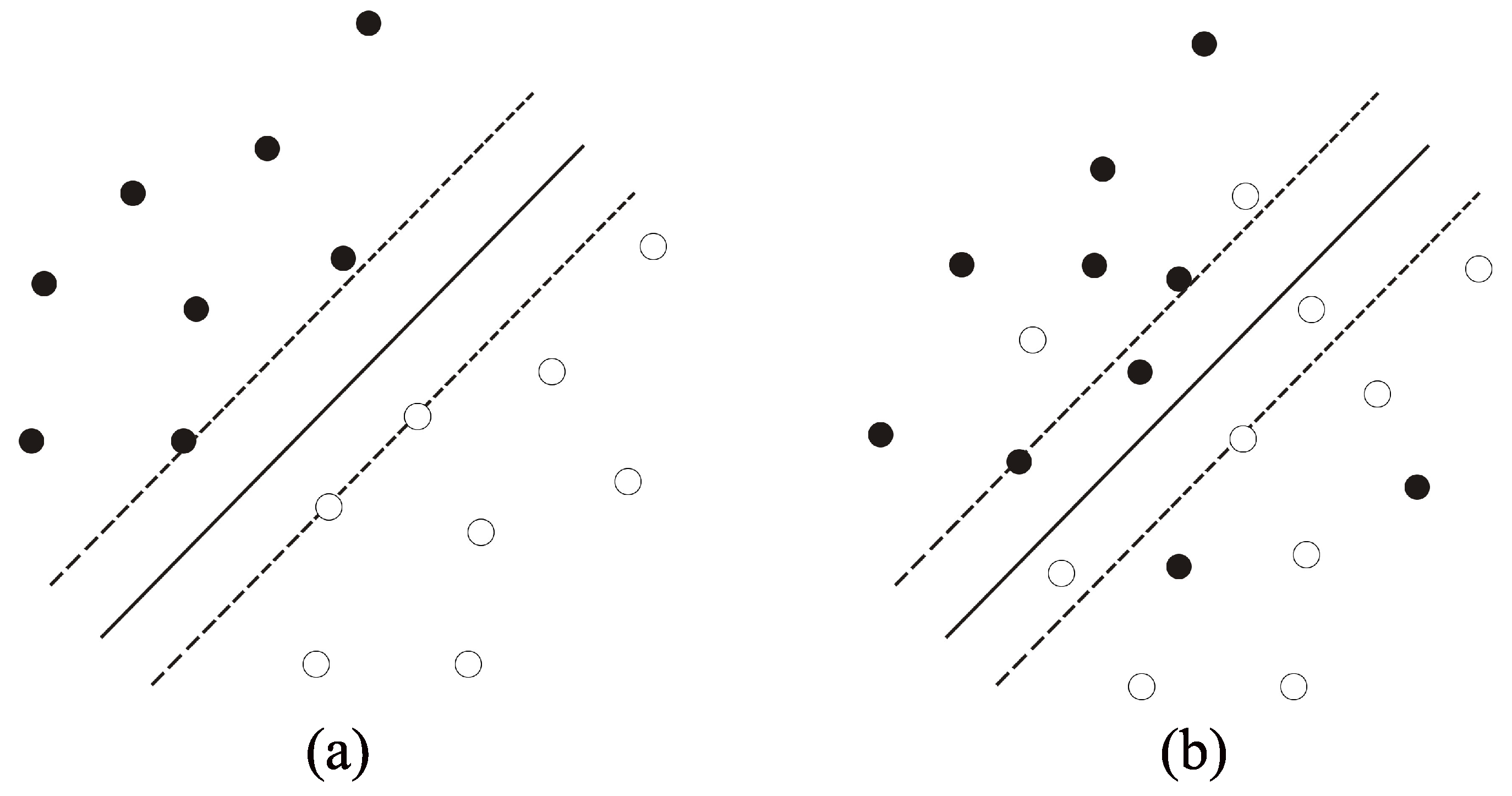
3.1. Support Vector Classifier
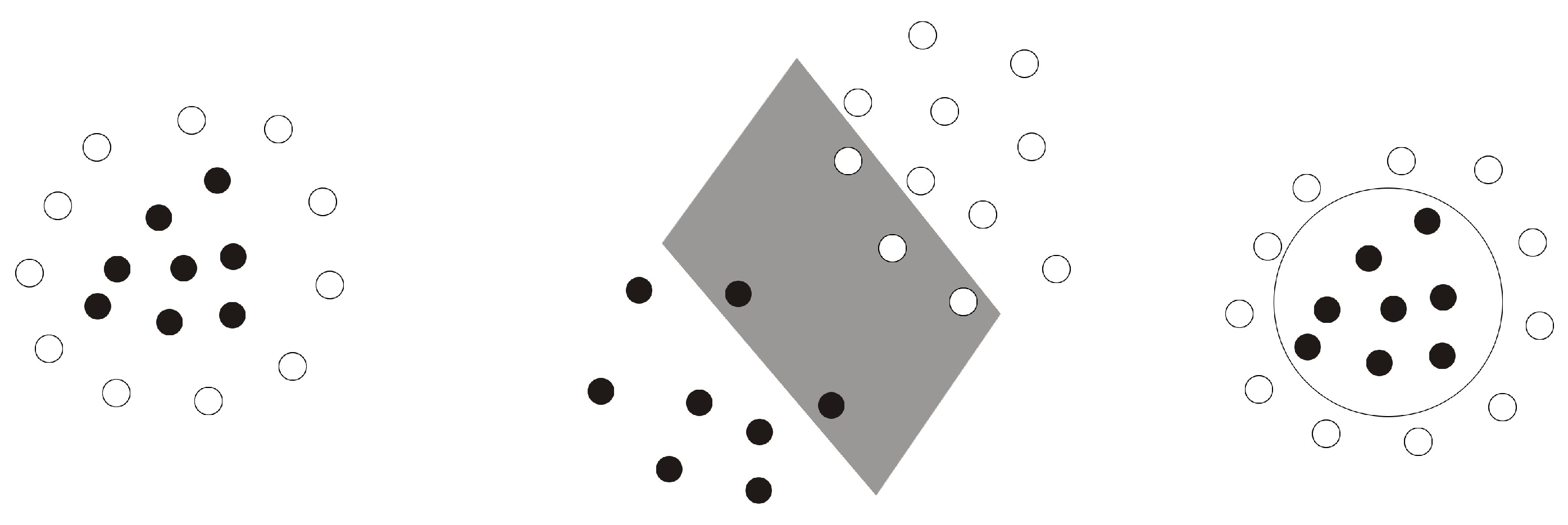
3.2. Kernel Transformation
3.3. Convolution Procedures and SVM
4. Simulation Study
Experimental Setup
- Accuracy (ACC): is the rate between correct predictions and total of predictions. It is sensitive to classes unbalancing.
- Sensitivity (SEN): known as recall, it is the rate of true positive predictions and all positive predictions.
- Specificity (SPC): it is the rate of true negative predictions and all negative predictions.
- Matthew’s correlation coefficient (MCC): this metric measures the correlation between true and predicted values. It may vary from −1 to 1 and the closer to 1 the correlation value is, the better is the predictions.
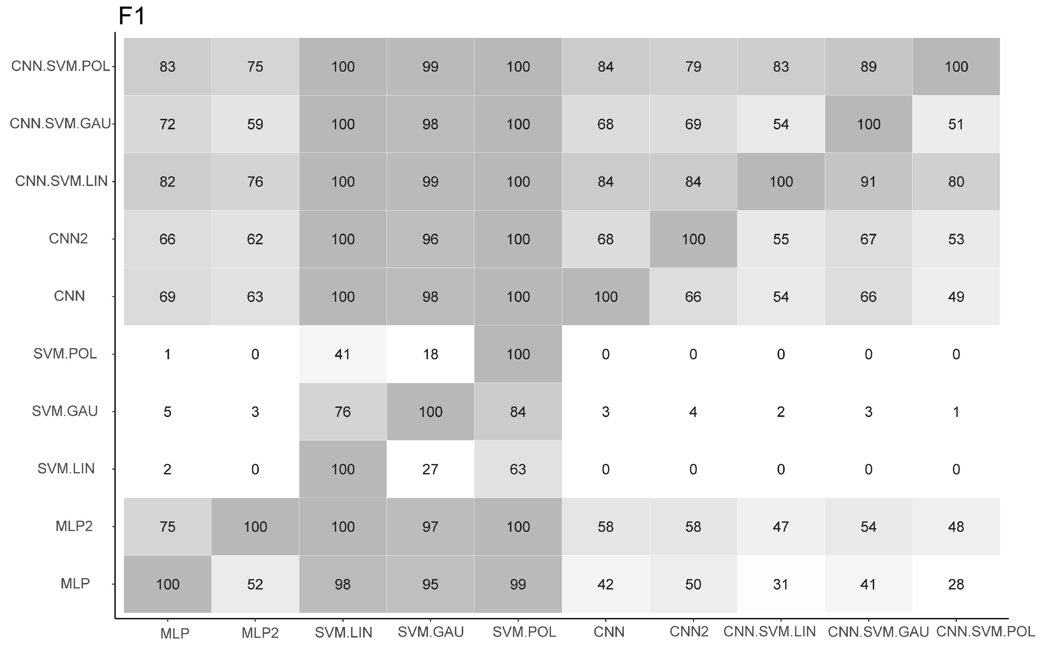
- F1 Score (F1): this metric is the harmonic mean of precision and recall. Precision indicates how many positive predictions are positive.
5. Real Data Study
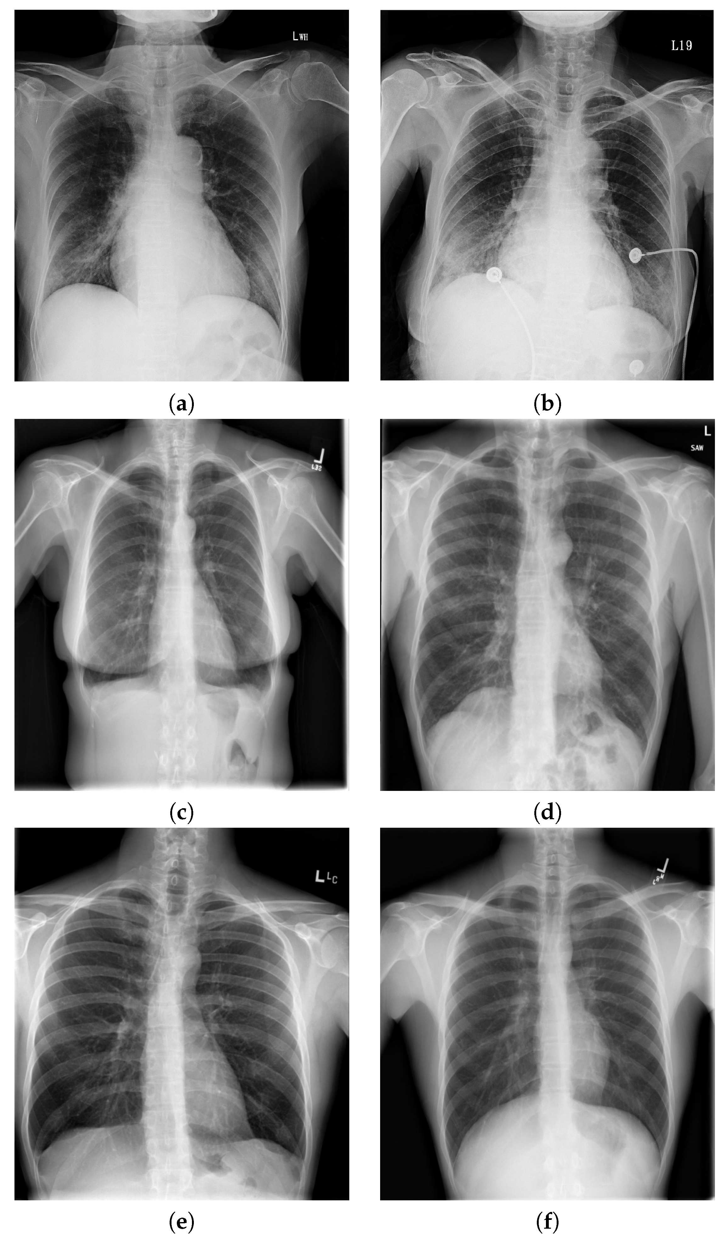
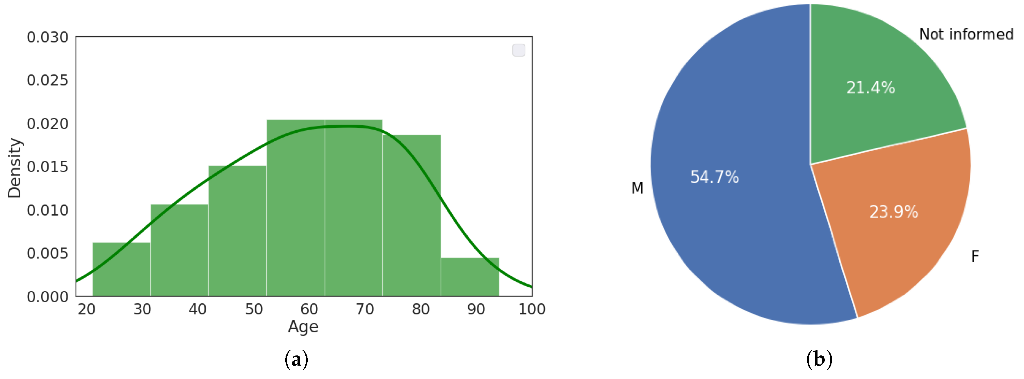
5.1. Data and X-ray Image Acquisition
5.2. Predictive Models
6. Final Considerations
Author Contributions
Funding
Conflicts of Interest
References
- Wang, C.; Horby, P.W.; Hayden, F.G.; Gao, G.F. A novel coronavirus outbreak of global health concern. Lancet 2020, 395, 470–473. [Google Scholar] [CrossRef]
- Dong, E.; Du, H.; Gardner, L. An interactive web-based dashboard to track COVID-19 in real time. Lancet Infect. Dis. 2020, 20, 533–534. [Google Scholar] [CrossRef]
- Korber, B.; Fischer, W.M.; Gnanakaran, S.; Yoon, H.; Theiler, J.; Abfalterer, W.; Hengartner, N.; Giorgi, E.E.; Bhattacharya, T.; Foley, B.; et al. Tracking changes in SARS-CoV-2 Spike: Evidence that D614G increases infectivity of the COVID-19 virus. Cell 2020, 182, 812–827. [Google Scholar] [CrossRef] [PubMed]
- Velavan, T.P.; Meyer, C.G. The COVID-19 epidemic. Trop. Med. Int. Health 2020, 25, 278. [Google Scholar] [CrossRef] [PubMed]
- Sun, P.; Lu, X.; Xu, C.; Sun, W.; Pan, B. Understanding of COVID-19 based on current evidence. J. Med. Virol. 2020, 92, 548–551. [Google Scholar] [CrossRef] [PubMed]
- Kim, J.Y.; Choe, P.G.; Oh, Y.; Oh, K.J.; Kim, J.; Park, S.J.; Park, J.H.; Na, H.K.; Oh, M.D. The first case of 2019 novel coronavirus pneumonia imported into Korea from Wuhan, China: Implication for infection prevention and control measures. J. Korean Med. Sci. 2020, 35, e61. [Google Scholar] [CrossRef]
- Zhang, G.; Wang, W.; Moon, J.; Pack, J.K.; Jeon, S.I. A review of breast tissue classification in mammograms. In Proceedings of the 2011 ACM Symposium on Research in Applied Computation, Taichung, Taiwan, 21–25 March 2011; pp. 232–237. [Google Scholar]
- El-Yaagoubi, M.; Mora-Jiménez, I.; Jabrane, Y.; Muñoz-Romero, S.; Rojo-Álvarez, J.L.; Pareja-Grande, J.A. Quantitative Cluster Headache Analysis for Neurological Diagnosis Support Using Statistical Classification. Information 2020, 11, 393. [Google Scholar] [CrossRef]
- Pellegrini, E.; Ballerini, L.; Hernandez, M.D.C.V.; Chappell, F.M.; González-Castro, V.; Anblagan, D.; Danso, S.; Muñoz-Maniega, S.; Job, D.; Pernet, C.; et al. Machine learning of neuroimaging for assisted diagnosis of cognitive impairment and dementia: A systematic review. Alzheimer’s Dement. Diagn. Assess. Dis. Monit. 2018, 10, 519–535. [Google Scholar] [CrossRef]
- Yassin, N.I.; Omran, S.; El Houby, E.M.; Allam, H. Machine learning techniques for breast cancer computer aided diagnosis using different image modalities: A systematic review. Comput. Methods Programs Biomed. 2018, 156, 25–45. [Google Scholar] [CrossRef]
- Asri, H.; Mousannif, H.; Al Moatassime, H.; Noel, T. Using machine learning algorithms for breast cancer risk prediction and diagnosis. Procedia Comput. Sci. 2016, 83, 1064–1069. [Google Scholar] [CrossRef]
- Safdar, S.; Zafar, S.; Zafar, N.; Khan, N.F. Machine learning based decision support systems (DSS) for heart disease diagnosis: A review. Artif. Intell. Rev. 2018, 50, 597–623. [Google Scholar] [CrossRef]
- Liu, S.; Wang, Y.; Yang, X.; Lei, B.; Liu, L.; Li, S.X.; Ni, D.; Wang, T. Deep learning in medical ultrasound analysis: A review. Engineering 2019, 5, 261–275. [Google Scholar] [CrossRef]
- Bakator, M.; Radosav, D. Deep learning and medical diagnosis: A review of literature. Multimodal Technol. Interact. 2018, 2, 47. [Google Scholar] [CrossRef]
- Shen, D.; Wu, G.; Suk, H.I. Deep learning in medical image analysis. Annu. Rev. Biomed. Eng. 2017, 19, 221–248. [Google Scholar] [CrossRef] [PubMed]
- Cortes, C.; Vapnik, V. Support Vector Networks. Mach. Learn. 1995, 20, 273–297. [Google Scholar] [CrossRef]
- Tzotsos, A.; Argialas, D. Support vector machine classification for object-based image analysis. In Object-Based Image Analysis; Springer: Berlin/Heidelberg, Germany, 2008; pp. 663–677. [Google Scholar]
- Song, Q.; Hu, W.; Xie, W. Robust support vector machine with bullet hole image classification. IEEE Trans. Syst. Man. Cybern. Part C Appl. Rev. 2002, 32, 440–448. [Google Scholar] [CrossRef]
- Chaplot, S.; Patnaik, L.M.; Jagannathan, N. Classification of magnetic resonance brain images using wavelets as input to support vector machine and neural network. Biomed. Signal Process. Control 2006, 1, 86–92. [Google Scholar] [CrossRef]
- Maulik, U.; Chakraborty, D. Remote Sensing Image Classification: A survey of support-vector-machine-based advanced techniques. IEEE Geosci. Remote Sens. Mag. 2017, 5, 33–52. [Google Scholar] [CrossRef]
- Islam, M.; Dinh, A.; Wahid, K.; Bhowmik, P. Detection of potato diseases using image segmentation and multiclass support vector machine. In Proceedings of the 2017 IEEE 30th Canadian Conference on Electrical and Computer Engineering (CCECE), Windsor, ON, Canada, 30 April–3 May 2017; pp. 1–4. [Google Scholar]
- Huang, F.J.; LeCun, Y. Large-scale Learning with SVM and Convolutional Nets for Generic Object Categorization. In Proceedings of the IEEE Computer Society Conference on Computer Vision and Pattern Recognition, New York, NY, USA, 17–22 June 2006; pp. 1–8. [Google Scholar]
- Şentaş, A.; Tashiev, İ.; Küçükayvaz, F.; Kul, S.; Eken, S.; Sayar, A.; Becerikli, Y. Performance evaluation of support vector machine and convolutional neural network algorithms in real-time vehicle type and color classification. Evol. Intell. 2020, 13, 83–91. [Google Scholar] [CrossRef]
- Chagas, P.; Souza, L.; Araújo, I.; Aldeman, N.; Duarte, A.; Angelo, M.; dos Santos, W.L.; Oliveira, L. Classification of glomerular hypercellularity using convolutional features and support vector machine. Artif. Intell. Med. 2020, 103, 101808. [Google Scholar] [CrossRef]
- Witoonchart, P.; Chongstitvatana, P. Application of structured support vector machine backpropagation to a convolutional neural network for human pose estimation. Neural Netw. 2017, 92, 39–46. [Google Scholar] [CrossRef] [PubMed]
- Zafar, R.; Malik, A.S.; Shuaibu, A.N.; ur Rehman, M.J.; Dass, S.C. Classification of fmri data using support vector machine and convolutional neural network. In Proceedings of the 2017 IEEE International Conference on Signal and Image Processing Applications (ICSIPA), Kuching, Malaysia, 12–14 September 2017; pp. 324–329. [Google Scholar]
- Li, M.; Han, C.; Fahim, F. Skin Cancer Diagnosis Based on Support Vector Machine and a New Optimization Algorithm. J. Med. Imaging Health Inform. 2020, 10, 356–363. [Google Scholar] [CrossRef]
- Ferreira, L.K.; Rondina, J.M.; Kubo, R.; Ono, C.R.; Leite, C.C.; Smid, J.; Bottino, C.; Nitrini, R.; Busatto, G.F.; Duran, F.L.; et al. Support vector machine-based classification of neuroimages in Alzheimer’s disease: Direct comparison of FDG-PET, rCBF-SPECT and MRI data acquired from the same individuals. Braz. J. Psychiatry 2018, 40, 181–191. [Google Scholar] [CrossRef] [PubMed]
- Kale, S.D.; Punwatkar, K.M. Texture analysis of ultrasound medical images for diagnosis of thyroid nodule using support vector machine. Int. J. Comput. Sci. Mob. Comput. 2013, 2, 71–77. [Google Scholar]
- Orru, G.; Pettersson-Yeo, W.; Marquand, A.F.; Sartori, G.; Mechelli, A. Using support vector machine to identify imaging biomarkers of neurological and psychiatric disease: A critical review. Neurosci. Biobehav. Rev. 2012, 36, 1140–1152. [Google Scholar] [CrossRef]
- Novitasari, D.C.R.; Hendradi, R.; Caraka, R.E.; Rachmawati, Y.; Fanani, N.Z.; Syarifudin, A.; Toharudin, T.; Chen, R.C. Detection of COVID-19 chest X-ray using support vector machine and convolutional neural network. Commun. Math. Biol. Neurosci. 2020, 2020. [Google Scholar] [CrossRef]
- Sethy, P.K.; Behera, S.K. Detection of coronavirus disease (covid-19) based on deep features. Preprints 2020, 030300. [Google Scholar] [CrossRef]
- Tayarani-N, M.H. Applications of Artificial Intelligence in Battling Against Covid-19: A Literature Review. Chaos Solitons Fractals 2020, 110338. [Google Scholar] [CrossRef]
- Chen, D.; Liu, F.; Li, Z. A Review of Automatically Diagnosing COVID-19 based on Scanning Image. arXiv 2020, arXiv:2006.05245. [Google Scholar]
- Nishio, M.; Noguchi, S.; Matsuo, H.; Murakami, T. Automatic classification between COVID-19 pneumonia, non-COVID-19 pneumonia, and the healthy on chest X-ray image: Combination of data augmentation methods in a small dataset. arXiv 2020, arXiv:2006.00730. [Google Scholar]
- Luz, E.J.D.S.; Silva, P.L.; Silva, R.; Silva, L.; Moreira, G.; Menotti, D. Towards an Effective and Efficient Deep Learning Model for COVID-19 Patterns Detection in X-ray Images. arXiv 2020, arXiv:2004.05717. [Google Scholar]
- Apostolopoulos, I.D.; Mpesiana, T.A. Covid-19: Automatic detection from x-ray images utilizing transfer learning with convolutional neural networks. Phys. Eng. Sci. Med. 2020, 43, 635–640. [Google Scholar] [CrossRef] [PubMed]
- Heidari, M.; Mirniaharikandehei, S.; Khuzani, A.Z.; Danala, G.; Qiu, Y.; Zheng, B. Improving the performance of CNN to predict the likelihood of COVID-19 using chest X-ray images with preprocessing algorithms. Int. J. Med. Inform. 2020, 144, 104284. [Google Scholar] [CrossRef] [PubMed]
- Cao, K.; Choi, K.N.; Jung, H.; Duan, L. Deep Learning for Facial Beauty Prediction. Information 2020, 11, 391. [Google Scholar] [CrossRef]
- Goodfellow, I.; Bengio, Y.; Courville, A. Deep Learning; MIT Press: Cambridge, MA, USA, 2016. [Google Scholar]
- Witten, I.H.; Frank, E.; Hall, M.A. Data Mining Practical Learning Tools and Techniques, 4rd ed.; Morgan Kaufmann: Burlington, MA, USA, 2017; pp. 417–466. [Google Scholar]
- Wang, B.; Sun, Y.; Xue, B.; Zhang, M. Evolving Deep Convolutional Neural Networks by Variable-length Particle Swarm Optimization for Image Classification. In Proceedings of the 2018 IEEE Congress on Evolutionary Computation (CEC), Rio de Janeiro, Brazil, 8–13 July 2018. [Google Scholar]
- Ciaburro, G.; Venkateswaran, B. Neural Networks with R; Packt Publishing: Birmingham, UK, 2017. [Google Scholar]
- Haykin, S. Neural Networks and Learning Machines, 3rd ed.; Pearson Education, Inc.: Upper Saddle River, NJ, USA, 2009. [Google Scholar]
- Nagi, J.; Di Caro, G.A.; Giusti, A.; Nagi, F.; Gambardella, L.M. Convolutional Neural Support Vector Machines: Hybrid visual pattern classifiers for multirobot systems. In Proceedings of the 2012 11th International Conference on Machine Learning and Applications, Boca Raton, FL, USA, 12–15 December 2012. [Google Scholar]
- Tang, Y. Deep Learning using Linear Support Vector Machines. arXiv 2015, arXiv:1306.0239. [Google Scholar]
- Vapnik, V.N. An overview of statistical learning theory. IEEE Trans. Neural Netw. 1999, 10, 988–999. [Google Scholar] [CrossRef]
- Wang, W.; Xu, Z.; Lu, W.; Zhang, X. Determination of the spread parameter in the Gaussian kernel for classification and regression. Neurocomputing 2003, 55, 643–663. [Google Scholar] [CrossRef]
- Yaohao, P. Support Vector Regression Aplicado à Previsão de Taxas de Câmbio. Master’s Thesis, Universidade de Brasilia, Brasilia, Brazil, 2016. [Google Scholar]
- Elangovan, M.; Sugumaran, V.; Ramachandran, K.; Ravikumar, S. Effect of SVM kernel functions on classification of vibration signals of a single point cutting tool. Expert Syst. Appl. 2011, 38, 15202–15207. [Google Scholar] [CrossRef]
- Yekkehkhany, B.; Safari, A.; Homayouni, S.; Hasanlou, M. A comparison study of different kernel functions for SVM-based classification of multi-temporal polarimetry SAR data. Int. Arch. Photogramm. Remote Sens. Spat. Inf. Sci. 2014, 40, 281. [Google Scholar] [CrossRef]
- Chen, H.; Chen, A.; Xu, L.; Xie, H.; Qiao, H.; Lin, Q.; Cai, K. A deep learning CNN architecture applied in smart near-infrared analysis of water pollution for agricultural irrigation resources. Agric. Water Manag. 2020, 240, 106303. [Google Scholar] [CrossRef]
- Sarmento, P.L. Avaliação de méTodos de Seleção de Amostras para Redução do Tempo de Treinamento do Classificador SVM. Master’s Thesis, INPE, Sao Jose dos Campos, Brazil, 2014. [Google Scholar]
- Krizhevsky, A.; Sutskever, I.; Hinton, G.E. ImageNet Classification with Deep Convolutional Neural Networks. In Proceedings of the NIPS 2012, Lake Tahoe, NV, USA, 3–6 December 2012; Volume 25, pp. 1097–1105. [Google Scholar]
- Baldi, P.; Brunak, S.; Chauvin, Y.; Andersen, C.A.; Nielsen, H. Assessing the accuracy of prediction algorithms for classification: An overview. Bioinformatics 2000, 16, 412–424. [Google Scholar] [CrossRef] [PubMed]
- Chollet, F.; Allaire, J. R Interface to Keras. 2017. Available online: https://github.com/rstudio/keras (accessed on 20 November 2020).
- Karatzoglou, A.; Smola, A.; Hornik, K.; Zeileis, A. kernlab—An S4 Package for Kernel Methods in R. J. Stat. Softw. 2004, 11, 1–20. [Google Scholar] [CrossRef]
- Caputo, B.; Sim, K.; Furesjo, F.; Smola, A. Appearance-based object recognition using SVMs: Which kernel should I use? In Proceedings of the NIPS Workshop on Statistical Methods for Computational Experiments in Visual Processing and Computer Vision, Vancouver, BC, Canada, 9–14 December 2002; Volume 2002. [Google Scholar]
- Radiopedia. Chest (AP Erect View). Available online: https://radiopaedia.org/articles/chest-ap-erect-view-1 (accessed on 15 August 2020).
- Cohen, J.P.; Morrison, P.; Dao, L.; Roth, K.; Duong, T.Q.; Ghassemi, M. COVID-19 Image Data Collection: Prospective Predictions Are the Future. arXiv 2020, arXiv:2006.11988. [Google Scholar]
- Tantithamthavorn, C.; McIntosh, S.; Hassan, A.E.; Matsumoto, K. An empirical comparison of model validation techniques for defect prediction models. IEEE Trans. Softw. Eng. 2016, 43, 1–18. [Google Scholar] [CrossRef]
- Blumer, A.; Ehrenfeucht, A.; Haussler, D.; Warmuth, M.K. Occam’s razor. Inf. Process. Lett. 1987, 24, 377–380. [Google Scholar] [CrossRef]
- Domingos, P. The role of Occam’s razor in knowledge discovery. Data Min. Knowl. Discov. 1999, 3, 409–425. [Google Scholar] [CrossRef]
- Osuna, E.; Freund, R.; Girosi, F. An improved training algorithm for support vector machines. In Neural Networks for Signal Processing VII, Proceedings of the 1997 IEEE Signal Processing Society Workshop, Amelia Island, FL, USA, USA, 24–26 September 1997; IEEE: Piscataway, NJ, USA, 1997; pp. 276–285. [Google Scholar]
- Downs, T.; Gates, K.E.; Masters, A. Exact simplification of support vector solutions. J. Mach. Learn. Res. 2001, 2, 293–297. [Google Scholar]
- Geebelen, D.; Suykens, J.A.; Vandewalle, J. Reducing the number of support vectors of SVM classifiers using the smoothed separable case approximation. IEEE Trans. Neural Netw. Learn. Syst. 2012, 23, 682–688. [Google Scholar] [CrossRef]
- Kim, H.; Nam, H.; Jung, W.; Lee, J. Performance analysis of CNN frameworks for GPUs. In Proceedings of the 2017 IEEE International Symposium on Performance Analysis of Systems and Software (ISPASS), Santa Rosa, CA, USA, 24–25 April 2017; pp. 55–64. [Google Scholar]
- Litjens, G.; Ciompi, F.; Wolterink, J.M.; de Vos, B.D.; Leiner, T.; Teuwen, J.; Išgum, I. State-of-the-art deep learning in cardiovascular image analysis. JACC Cardiovasc. Imaging 2019, 12, 1549–1565. [Google Scholar] [CrossRef]
- Pound, M.P.; Atkinson, J.A.; Townsend, A.J.; Wilson, M.H.; Griffiths, M.; Jackson, A.S.; Bulat, A.; Tzimiropoulos, G.; Wells, D.M.; Murchie, E.H.; et al. Deep machine learning provides state-of-the-art performance in image-based plant phenotyping. Gigascience 2017, 6, gix083. [Google Scholar] [CrossRef]
- Mazurowski, M.A.; Buda, M.; Saha, A.; Bashir, M.R. Deep learning in radiology: An overview of the concepts and a survey of the state of the art with focus on MRI. J. Magn. Reson. Imaging 2019, 49, 939–954. [Google Scholar] [CrossRef] [PubMed]
- Cheng, G.; Han, J.; Lu, X. Remote sensing image scene classification: Benchmark and state of the art. Proc. IEEE 2017, 105, 1865–1883. [Google Scholar] [CrossRef]


| Kernel Type | Parameters | |
|---|---|---|
| Linear | ||
| Polynomial | ||
| Gaussian |
| Class 1 | Class 2 | |||
|---|---|---|---|---|
| Difference | Channel | |||
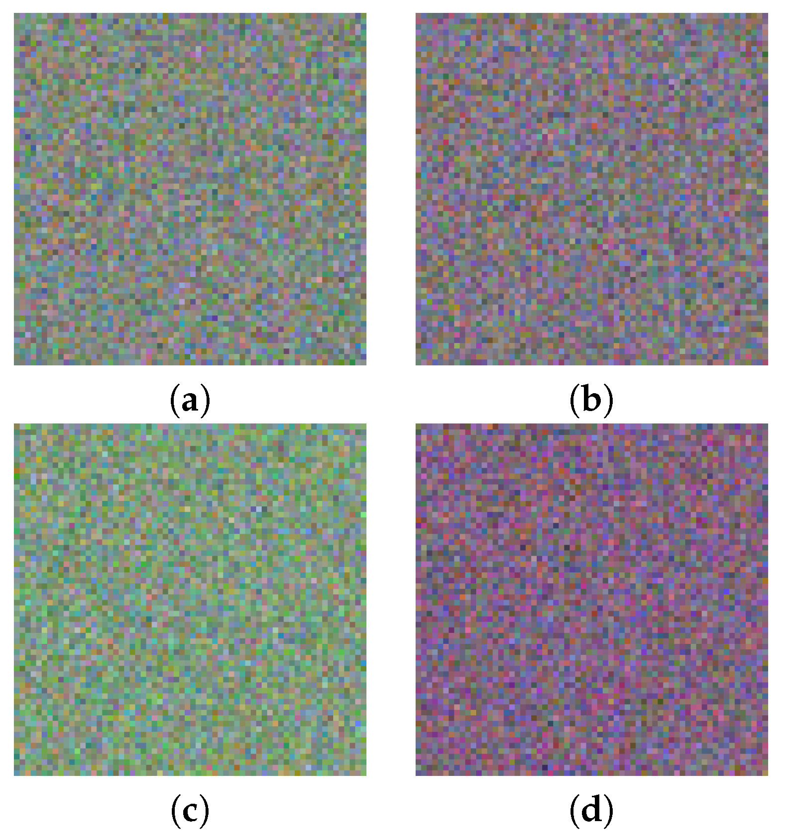
| R | 128 | 128 | 25 | |
| 1SD | G | 119 | 137 | 18 |
| B | 128 | 128 | 30 | |
| R | 128 | 128 | 25 | |
| 3SD | G | 101 | 155 | 18 |
| B | 128 | 128 | 30 | |
| Samples | Method | ACC | SEN | SPC | MCC | F1 | Time |
|---|---|---|---|---|---|---|---|
| CSVM | 0.46 | 0.40 | 0.51 | −0.10 | 0.45 | 0.09 | |
| CSVM | 0.45 | 0.41 | 0.49 | −0.10 | 0.44 | 0.09 | |
| 100 | CSVM | 0.45 | 0.41 | 0.49 | −0.10 | 0.45 | 0.09 |
| CNN | 0.49 | 0.23 | 0.75 | −0.04 | 0.50 | 0.12 | |
| CNN | 0.49 | 0.11 | 0.88 | −0.08 | 0.47 | 0.24 | |
| CSVM | 0.52 | 0.50 | 0.54 | 0.05 | 0.50 | 0.10 | |
| CSVM | 0.54 | 0.54 | 0.54 | 0.08 | 0.53 | 0.10 | |
| 300 | CSVM | 0.54 | 0.55 | 0.53 | 0.08 | 0.54 | 0.10 |
| CNN | 0.51 | 0.48 | 0.55 | 0.03 | 0.49 | 0.20 | |
| CNN | 0.50 | 0.08 | 0.91 | −0.07 | 0.40 | 0.53 | |
| CSVM | 0.88 | 0.88 | 0.88 | 0.77 | 0.88 | 0.13 | |
| CSVM | 0.88 | 0.87 | 0.88 | 0.76 | 0.88 | 0.12 | |
| 500 | CSVM | 0.87 | 0.86 | 0.88 | 0.74 | 0.87 | 0.12 |
| CNN | 0.87 | 0.85 | 0.88 | 0.74 | 0.86 | 0.27 | |
| CNN | 0.50 | 0.01 | 0.99 | 0.29 | 0.70 | 0.87 | |
| CSVM | 0.98 | 0.98 | 0.98 | 0.97 | 0.98 | 0.24 | |
| CSVM | 0.98 | 0.98 | 0.99 | 0.97 | 0.98 | 0.20 | |
| 1000 | CSVM | 0.98 | 0.98 | 0.98 | 0.97 | 0.98 | 0.22 |
| CNN | 0.99 | 0.99 | 0.99 | 0.98 | 0.99 | 0.50 | |
| CNN | 0.77 | 0.55 | 0.98 | 0.93 | 0.97 | 2.46 |
| Samples | Method | ACC | SEN | SPC | MCC | F1 | Time |
|---|---|---|---|---|---|---|---|
| CSVM | 0.45 | 0.41 | 0.49 | −0.10 | 0.45 | 0.09 | |
| CSVM | 0.44 | 0.43 | 0.45 | −0.13 | 0.45 | 0.10 | |
| 100 | CSVM | 0.44 | 0.42 | 0.46 | −0.12 | 0.45 | 0.10 |
| CNN | 0.48 | 0.22 | 0.74 | −0.13 | 0.50 | 0.13 | |
| CNN | 0.50 | 0.16 | 0.84 | −0.12 | 0.56 | 0.24 | |
| CSVM | 0.51 | 0.54 | 0.47 | 0.02 | 0.52 | 0.10 | |
| CSVM | 0.51 | 0.51 | 0.50 | 0.19 | 0.51 | 0.10 | |
| 300 | CSVM | 0.51 | 0.52 | 0.51 | 0.03 | 0.51 | 0.10 |
| CNN | 0.51 | 0.48 | 0.53 | 0.02 | 0.48 | 0.21 | |
| CNN | 0.49 | 0.17 | 0.82 | −0.02 | 0.38 | 0.54 | |
| CSVM | 0.88 | 0.88 | 0.88 | 0.78 | 0.88 | 0.12 | |
| CSVM | 0.89 | 0.89 | 0.89 | 0.79 | 0.89 | 0.11 | |
| 500 | CSVM | 0.90 | 0.89 | 0.90 | 0.80 | 0.90 | 0.11 |
| CNN | 0.89 | 0.89 | 0.89 | 0.79 | 0.89 | 0.28 | |
| CNN | 0.88 | 0.87 | 0.90 | 0.80 | 0.89 | 0.95 | |
| CSVM | 1.00 | 1.00 | 1.00 | 1.00 | 1.00 | 0.18 | |
| CSVM | 1.00 | 1.00 | 1.00 | 1.00 | 1.00 | 0.16 | |
| 1000 | CSVM | 1.00 | 1.00 | 1.00 | 1.00 | 1.00 | 0.16 |
| CNN | 1.00 | 1.00 | 1.00 | 1.00 | 1.00 | 0.48 | |
| CNN | 0.99 | 0.99 | 1.00 | 1.00 | 1.00 | 2.65 |
| COVID-19 | Other Diseases | Healthy | Total | |
|---|---|---|---|---|
| Quantity | 217 | 108 | 112 | 437 |
| Method | ACC | F1 | MCC | Time |
|---|---|---|---|---|
| MLP | 95.54 | 95.46 | 91.57 | 0.0422 |
| MLP | 96.59 | 96.56 | 93.48 | 0.0370 |
| CNN | 96.67 | 96.63 | 93.48 | 0.7792 |
| CNN | 96.73 | 96.67 | 93.74 | 0.7585 |
| SVM | 80.79 | 80.21 | 61.98 | 0.0074 |
| SVM | 77.90 | 77.24 | 56.30 | 0.0076 |
| SVM | 83.45 | 83.86 | 67.39 | 0.0067 |
| CSVM | 98.00 | 97.97 | 96.11 | 0.0146 |
| CSVM | 96.57 | 98.13 | 96.36 | 0.0143 |
| CSVM | 98.14 | 96.59 | 93.34 | 0.0151 |
Publisher’s Note: MDPI stays neutral with regard to jurisdictional claims in published maps and institutional affiliations. |
© 2020 by the authors. Licensee MDPI, Basel, Switzerland. This article is an open access article distributed under the terms and conditions of the Creative Commons Attribution (CC BY) license (http://creativecommons.org/licenses/by/4.0/).
Share and Cite
Maia, M.; Pimentel, J.S.; Pereira, I.S.; Gondim, J.; Barreto, M.E.; Ara, A. Convolutional Support Vector Models: Prediction of Coronavirus Disease Using Chest X-rays. Information 2020, 11, 548. https://doi.org/10.3390/info11120548
Maia M, Pimentel JS, Pereira IS, Gondim J, Barreto ME, Ara A. Convolutional Support Vector Models: Prediction of Coronavirus Disease Using Chest X-rays. Information. 2020; 11(12):548. https://doi.org/10.3390/info11120548
Chicago/Turabian StyleMaia, Mateus, Jonatha S. Pimentel, Ivalbert S. Pereira, João Gondim, Marcos E. Barreto, and Anderson Ara. 2020. "Convolutional Support Vector Models: Prediction of Coronavirus Disease Using Chest X-rays" Information 11, no. 12: 548. https://doi.org/10.3390/info11120548
APA StyleMaia, M., Pimentel, J. S., Pereira, I. S., Gondim, J., Barreto, M. E., & Ara, A. (2020). Convolutional Support Vector Models: Prediction of Coronavirus Disease Using Chest X-rays. Information, 11(12), 548. https://doi.org/10.3390/info11120548