Article

Least Squares Consensus for Matching Local Features

1
School of Automation Science and Engineering, South China University of Technology, Guangzhou 510641, Guangdong, China
2
School of Data Science and Information Engineering, Guizhou Minzu University, Guiyang 550025, Guizhou, China
3
School of Robot Engineering, Yangtze Normal University, Chongqing 408100, Chongqing, China
*
Authors to whom correspondence should be addressed.
Information 2019, 10(9), 275; https://doi.org/10.3390/info10090275
Submission received: 23 July 2019 / Revised: 28 August 2019 / Accepted: 28 August 2019 / Published: 2 September 2019

Abstract

:
This paper presents a new approach to estimate the consensus in a data set. Under the framework of RANSAC, the perturbation on data has not been considered sufficiently. We analysis the computation of homography in RANSAC and find that the variance of its estimation monotonically decreases when the size of sample increases. From this result, we carry out an approach which can suppress the perturbation and estimate the consensus set simultaneously. Different from other consensus estimators based on random sampling methods, our approach builds on the least square method and the order statistics and therefore is an alternative scheme for consensus estimation. Combined with the nearest neighbour-based method, our approach reaches higher matching precision than the plain RANSAC and MSAC, which is shown in our simulations.

1. Introduction

The random sample consensus (RANSAC) [1] has been broadly applied to obviate outliers with the nearest neighbour-based approach (NNA) for matching features. It prominently increases the precision-recall rate of matches. Under the framework of RANSAC, many improved versions have been studied. Using maximum likelihood estimation (MLE) instead of counting inliers, MLESAC introduces a likelihood function to evaluate a consensus set [2]. AMLESAC also exploits the MLE technique in consensus estimation but, other than MLESAC, only estimating outlier share in its procedure, AMLESAC estimates outlier share and inlier noise simultaneously [3]. To speed up the computation of RANSAC, R-RANSAC applies a preliminary test procedure, which evaluates the hypotheses by a small-sized sample to reduce some unnecessary verifications against all data points [4]. Exploiting Wald’s sequential probability test (SPRT), the optimal R-RANSAC also employs the preliminary test scheme to improve RANSAC [5]. Rather than the “depth-first” scheme in RANSAC, the preemptive RANSAC adopts the “breadth-first” strategy, which first generates all hypotheses and then compares them [6]. Guided-MLESAC uses a distribution constructed by the prior information instead of the uniform distribution, which generates hypotheses with a higher probability for searching the largest consensus set [7]. Unlike the plain RANSAC uniformly generating hypotheses, PROSAC non-uniformly draws samples from a sequence of monotonically increasing subsets, which are ordered by some “quality” valued by the element with the worst likely score in each subset. This scheme enables uncontaminated correspondences to be drawn as early as possible, thus reducing computational cost [8]. SEASAC further improves PROSAC through updating samples with only one data point at a time, replacing the worst one, whereas any such points in PROSAC will not be removed [9]. Cov-RANSAC employs SPRT and covariance test to form a set of potential inliers, on which the standard RANSAC run afterwards [10]. Before the procedure of RANSAC, DT-RANSAC constructs a refined set from putative matches based on topological information [11]. Since the scale ratio of correct matches approximates the scale variation of two images, SVH-RANSAC proposes a scale constraint, the scale variation homogeneity, to group data points, and thus the potential correct matches are more probable to be used to generate hypotheses [12]. SC-RANSAC exploits matching score to produce a set of reliable data points and then generates a hypothesis from these data points [13].
In the standard RANSAC framework, all inliers are treated as having equal quality for hypothesizing homographies and, by this assumption, the number of times attempting to obtain the largest consensus set is estimated. Then the noise in inliers can affects the precision of estimating homographies and therefore impacts on the estimation of the largest consensus set. To cope with this defect, we study an approach of consensus estimation suppressing the influence from noise. The rest of this work is organized as follows. In Section 2, we discuss the limitation and some improvements in the standard RANSAC framework on the noise problem. In Section 3, we present a new approach for consensus estimation, which is based on the least square method. In Section 4, a new feature matching method built on our new consensus estimator is presented. In Section 5, we test the least square based consensus estimator and compare it with the plain RANSAC and MSAC. Finally we conclude our work in Section 6.

2. The Limitation and Improvements on the RANSAC in Matching Features

Denote by X a finite set consisting of inliers and outliers. We define here inliers as the data points satisfying a specified homography and ouliers as the data points not satisfying the homography. Denote by G the set consisting of samples drawn from X . The sizes of samples in X are no less than N 0 , the least number for calculating the homography. We call an element in G a generator. Then each generator corresponds to a homograhpy [14]. Denote by H the set consisting of all homographies corresponding to generators in G . Then there exists a homography which most approximates the specified homography and we denote it by H o . In the problem of matching features, the homography between images is in general unknown. If the homography is estimated precisely, i.e., choosing a homography H from H approximating H o as much as possible, then by H many erroneous matches can be obviated. The standard RANSAC framework can be seen as a Bernoulli process [14]. In each Bernoulli trial, a homography H i is drawn from H through computation of using a random sample drawn from G . The drawn sample is denoted by G i correspondingly. Then the homograhpy H determines a set of data points, which is a subset of X and denoted by X G i . The set X G i is called the consensus set of G i [1]. Obviously, the consensus set corresponding to H o , which is denoted by X o here, is the set most approximating the set consisting of true matches. We call the consensus set X o the ideal consensus set. When the RANSAC is employed for matching features, the largest set in consensus sets, X * = a r g m a x i X G i , is the solution to the problem. X * is called the largest consensus set [1] and its optimal solution is the ideal consensus set X o .
The direct linear transformation (DTL) is usually applied to compute the homography between two images and it underlies consensus estimation. Suppose that H is the homography between two images and Y = ( y 1 , y 2 , 1 ) T , X = ( x 1 , x 2 , 1 ) T are two points in the images respectively, satisfying Y = H X . Considering there existing perturbation, we introduce some noise of zero mean value into this model,
y 1 y 2 1 = H x 1 x 2 1 + ϵ 1 ϵ 2 0 .
Denote entries in H by h i , namely, H = h 1 h 2 h 3 h 4 h 5 h 6 h 7 h 8 h 9 and set h 9 = 1 . Hence it is easy to obtain that
y 1 y 2 = x 1 x 2 1 0 0 0 x 1 y 1 x 2 y 1 0 0 0 x 1 x 2 1 x 1 y 2 x 2 y 2 h 1 h 2 h 3 h 4 h 5 h 6 h 7 h 8 + ϵ 1 ϵ 2 .
Suppose that there are N pairs of corresponding points, { X i } i = 1 N and { Y i } i = 1 N . Set X i = ( x 1 i , x 2 i , 1 ) T , Y i = ( y 1 i , y 2 i , 1 ) T and denote by ( ϵ 1 i , ϵ 1 i , 0 ) T the perturbation on the i-th corresponding point. Then we have
Q = ( P 1 , , P 8 ) h + ε ,
where Q = ( y 1 1 , y 2 1 , , y 1 N , y 2 N ) T , h = ( h 1 , , h 8 ) T , ε = ( ϵ 1 1 , ϵ 2 1 , , ϵ 1 N , ϵ 2 N ) T and
( P 1 , , P 8 ) = x 1 1 x 2 1 1 0 0 0 x 1 1 y 1 1 x 2 1 y 1 1 0 0 0 x 1 1 x 2 1 1 x 1 1 y 2 1 x 2 1 y 2 1 x 1 N x 2 N 1 0 0 0 x 1 N y 1 N x 2 N y 1 N 0 0 0 x 1 N x 2 N 1 x 1 N y 2 N x 2 N y 2 N .
Therefore provided the rank of the matrix ( P 1 , , P 8 ) is no less than 8, the homography H can be estimated by Equation (1) and particularly when the rank is greater than 8, the least squares estimation (LSE) can be applied to compute the homography H.
Proposition 1.
Suppose v a r ( Q ) = σ 2 I N . When using (1) to estimate the h, a larger sample size of corresponding points entails a more precise estimation.
Proof. 
It is not difficult to know
v a r ( h ) = σ 2 ( ( P 1 , , P 8 ) T ( P 1 , , P 8 ) ) 1 ,
which means that with more elements in each P i ( i = 1 , , 8 ) , the elements in the principal diagonal of v a r ( h ) tend to be smaller and therefore the estimation of h tends to be more effective. □
Nevertheless directly adopting a large number of corresponding points to estimate consensus under the standard RANSAC framework is difficult, which can be justified by the following fact. Suppose that n is the number of all candidates and n I is the number of all inliers. If there are N (which should not be greater than n I ) corresponding points being employed to calculate a homography, then the probability that all these N corresponding points are inliers is
P N = n I N n N = n I ! ( n N ) ! n ! ( n I N ) ! = n I ! n ! ( n N ) ( n I N + 1 ) ,
Assume that N 1 and N 2 are two numbers of corresponding points for computing a homography, satisfying N 2 = N 1 + m , m > 0 . Then we have
P N 2 P N 1 = i = n I + 1 n ( i N 1 m ) i = n I + 1 n ( i N 1 ) = i = 1 m n I N 1 i + 1 n N 1 i + 1 < ( n I n ) m ,
which means that in such a Bernoulli trial, for the event that all data points in the sample of N 2 size are inliers to occur, under the same given probability, the number of attempts is at least as many as ( n n I ) m times for the event that all data points in the sample of N 1 size are inliers to occur. Therefore when the n I is relatively small (e.g., n I < 0.5 n ), the cost to reduce the influence from noise under the standard RANSAC framework is enormous (e.g., the cost for reducing noise is 2 m times greater than ignoring noise).
Some works for reducing the influence of the noise have been carried out. Torr et al. proposes that inliers are not equal in quality, different from the assumption in the standard RANSAC [2]. The unequal quality amid inliers is caused by perturbation added in data points. From this perspective, The different scores for inliers are introduced in MSAC and in MLESAC, MLE is exploited instead of the cardinality of the consensus set to value the fitness between the hypothetical homographies and the true homography and therefore to lower the influence from noise. Chum et al. embeds a local optimization procedure into the standard RANSAC framework, which only runs when a new maximal consensus set of inliers is found. This consensus set then is applied to compute a new hypothetical homography [15]. Therefore the new hypothetical homography is always estimated by generators with increasing size. In term of Proposition 1, the local-optimization-embedded RANSAC is more effective than the standard RANSAC in the estimation on the consensus. İmre et al. introduce order statistics into discussions on RANSAC, regarding the estimation of consensus as the estimation of the first order statistic. Then the Top-n criterion is presented to determine the times of Bernoulli trials [14]. Since RANSAC assumes no perturbation in data and thus pragmatically the termination criterion does not ensure to obtain a consensus set approximating the largest consensus set enough. The Top-n criterion in fact admits the existence of noise in data. Consequently, under a given confidence, the method with the Top-n criterion can obtain the solution which arbitrarily approximates the homography corresponding to the largest consensus set. However, although these approaches have taken account of the perturbation in data, the only one able to obtain the solution approximating the ideal consensus set is the Lo-RANSAC [15]. Our aim is also to present a method which can obtain the solution approximating the ideal consensus set but different from the Lo-RANSAC, our method is not under the standard RANSAC framework but based on Proposition 1 and the LSE estimates the consensus while depressing the influence from noise simultaneously.

3. A Least Squares Consensus Estimation

By Equation (2), we can carry out the following result.
Proposition 2.
Suppose { X i } i = 1 a sequence of data points and { H i } i = 1 a sequence of homographies estimated from { X i } i = 1 where H i is estimated by { X 1 , , X i } . Then the sequence { v a r ( H i ) } i = 1 monotonically decreases if an arbitrary X { X i } i = 1 is an inlier.
This proposition can be used to rule out outliers if we have prior known some inliers in the set. Assume that G is a subset of X and all elements in it are inliers. If a new data point from X is added into G and a new hypothetical homography derived by this new generator gives a smaller consensus set, that is, the estimation of the new hypothetical homography being more deviated to the true value, then it is reasonable to deem the new added data point to be an outlier with large probability. Hence we propose a method of consensus estimation which iteratively computes the LSE, not only eliminating outliers but also diminishing the influence from the noise. The pivot step for this new method is to find a necessary subset consisting of inliers to be used in LSE.
We introduce the information of descriptors to obtain this pivot subset and define the Euclidean distance between two descriptors as the distance measurement of their corresponding features. It can be seen from precision-recall curves of some classical descriptors, such as SIFT, SURF and so forth, that matches with smaller distance measurements are more likely to be inliers in putatively matched local features [16,17,18,19]. Heuristically, we have
Pr ( the match X is true ) Pr ( the distance measurement of the match X is less than a small value ) .
Regard each element in X as a sample drawn from some population and denote these samples by X 1 , , X n . We construct the order statistics on these samples as
( X ( 1 ) , , X ( n ) ) ,
where X ( i ) is with the i-th smallest value of distance measurement in X 1 , , X n . Let d 0 be a variable of distance measurements and D ( · ) be a function on the set of all putative matches:
D : X R 0 ,
representing the distance measurement of a putative match. Therefore, once X 1 , , X n are drawn, each D ( X i ) ( i = 1 , , n ) is a random variable. Herefrom we denote D ( X i ) by D i and introduce the following result from Reference [14] directly.
Proposition 3
(Theorem 1, [14]). Suppose A ( d ) is a cumulative distribution function of the random variable D. Let D 1 , , D n be i.i.d. random variables drawn from D and ( D ( 1 ) , , D ( n ) ) be order statistics, where D ( i ) is the i-th smallest value of D 1 , , D n . The probability that the i-th order statistic is smaller than or equal to d is
Pr ( D ( i ) d ) = k = i I I k A ( d ) k ( 1 A ( d ) ) ( I k ) .
The above proposition yields that
Pr ( D ( i ) d ) = I k A k ( d ) ( 1 A ( d ) ) I k + Pr ( D ( i + 1 ) d ) .
The Equation (4) means that given a small permitted distance, a putative match corresponding to a distance measurement with a smaller rank in the order statistics ( D ( 1 ) , , D ( I ) ) is more likely to be a true match. Hence we apply the order statistics Equation (3) to compute LSE. Initially, the first k (which should not be less than 4 when calculating a homography matrix [10]) order statistics are used to be an initial generator. Then exploiting Proposition 2 through the sequence Equation (3) rules out outliers. When each order statistic in Equation (3) has been sifted, a sample of large size can be obtained. By Proposition 1, this sample can be employed to get an estimation more effective than the sample of smaller size used in the standard RANSAC and yield a set of matches approximating the ideal consensus set. Since the LSE is applied to estimate the consensus, we add the least squares consensus estimate (LESC) to the new method.

4. Matching Features by LESC

Since the minimal number of matches for computing a homography is 4, the putative matches with ranks from 1 to 4 are applied to generate the first hypothetical homography. Denote by G i the i-th generator, by H i the i-th hypothetical homograhy generated by G i through the LSE and by C i the i-th consensus set computed by H i from X . For convenience, we define the set of the first four order statistics to be the generator G 4 . Thus at the initial step the hypothetical homography and the consensus set are H 4 and C 4 respectively. Once G i , H i and C i are obtained, a test and approximation scheme is carried out as follows:
(a)
Add a new element to G i to speculate a new generator
G ˜ i + 1 = G i { x ( i + 1 ) } .
(b)
Compute a new hypothetical homography H ˜ i + 1 through the LSE by G ˜ i + 1 .
(c)
Compute a new consensus set C ˜ i + 1 from X by H ˜ i + 1 . A threshold T for considering inliers is exploited here. A match ( a , b ) is considered an element in the set C ˜ i + 1 if and only if it satisfies
b h ˜ i + 1 a < T 2 ,
where a and b are points in two planar images respectively and h ˜ i + 1 is a 2-dimensional transformation matrix derived from H ˜ i + 1 .
(d)
Compare the cardinality of C i and C ˜ i + 1 . If the cardinality of C ˜ i + 1 is larger, then put
G i + 1 = G ˜ i + 1 , H i + 1 = H ˜ i + 1 , C i + 1 = C ˜ i + 1 ,
otherwise put
G i + 1 = G i , H i + 1 = H i , C i + 1 = C i .
(e)
Repeat (a)∼(d) until the largest order statistic X ( n ) has been processed through above steps.
When these iterations are finished, the homography H n and the consensus set C n are the solutions and elements in C n are matched features. Since the noise is suppressed in the procedure of estimating the homography H n , the obtained consensus set approximates the ideal consensus set more than the largest consensus set does in RANSAC.
Since all elements in X are employed to tentatively put into the generator, the cost for unnecessary computation may severely increase when the size of X is large and the inliers is fairly small. To cope with this defect, we weigh up the reduction of elapsed time and the number of recalls. According to Proposition 3, an element with higher rank in the order statistics is less probable to be an inlier than one with lower rank. Therefore the frequency of inliers in some ordered data points is an upper bound of the probability that a data point with rank higher than the ranks of these ordered data points is an inlier. We can exploit this result to add a control scheme into above method to trade off the cost of computation time and the number of recalls. Simply calculating the ratio of inliers, namely
r = | G i + 1 | i + 1 ,
can value that upper bound. Then we assign a parameter as a threshold. Once the current ratio of inliers is less than the threshold, the procedure of producing generators and finding inliers stops.
We summarize the schemes above as the Algorithm of LESC shown in Algorithm 1.
Algorithm 1 The Least Squares Consensus Estimation
Input: The order statistics x ( 1 ) , , x ( I ) as defined by Equation (3), and the parameter R.
Produce the initial generating set G 4 = { x ( 1 ) , x ( 2 ) , x ( 3 ) , x ( 4 ) } , the initial hypothetical homography H 4 and the initial consensus set C 4 .
for i = 5 : n
(a)
Produce a speculated generating set G ˜ i by Equation (5).
(b)
Compute a new hypothetical homography by G ˜ i through the LSE;
(c)
Compute a new consensus set C ˜ i from X by H ˜ i according to Equation (6);
(d)
Obtain the current consensus set C i by Equation (7) or (8);
(e)
Calculate the ratio of inliers r by Equation (9) and if r < R then break;
end for
Output: A set of true matches C i .

5. Simulations and Results

We employ four methods, NNA, NNA with the plain RANSAC (NNA-RANSAC), NNA with the MSAC (NNA-MSAC) and NNA with LESC (NNA-LESC), to compute their performance of precision versus the number of recalls by Mikolajczyk’s criteria [20] (The image sequences are from the website http://www.robots.ox.ac.uk/∼vgg/research/affine/.). The codes of RANSAC and MSAC adopted in our simulations are developed by Marco Zuliani (All these codes are downloaded from the website https://github.com/RANSAC/RANSAC-Toolbox.). We set the threshold T in Equation (6) to be 3 pixels. The parameters of RANSAC are the same as MSAC, which are given in Table 1. The threshold R in Algorithm 1 is changed according to the sequence: { 0 , 0.01 , 0.02 , 0.05 , 0.1 } and experiments are run repeatedly at each setting of R. Our simulating environment is Windows 7 (64 bits) on the CPU of i7-5550U(2.00G) and the RAM of 16 G.
For extracting and describing local features, the SURF [18,19] algorithm is adopted, for which we utilize the codes all from OpenSURF originally developed by Chris Evans (the original codes are downloaded from the website https://github.com/gussmith23/opensurf.). First, we use SURF to extract local features and to describe them through all test images. Second, we match features in the first image to the rest of images in each test group by NNA, NNA-RANSAC, NNA-MSAC and NNA-LESC, respectively. The results of the experiment in which the parameter R of LESC is 0.01 are shown in Figure 1, Figure 2, Figure 3, Figure 4, Figure 5, Figure 6, Figure 7 and Figure 8. In term of results of simulations, when the threshold R is small enough, the number of recalls reduces slowly while the cost of the computation time decreases rapidly. An example depicts this outcome, which can be seen from Table 2, where the data are obtained through using Algorithm 1 on the first image versus the second image in the Lueven sequence at settings of R: 0 , 0.01 , 0.02 , 0.05 and 0.1 , respectively.
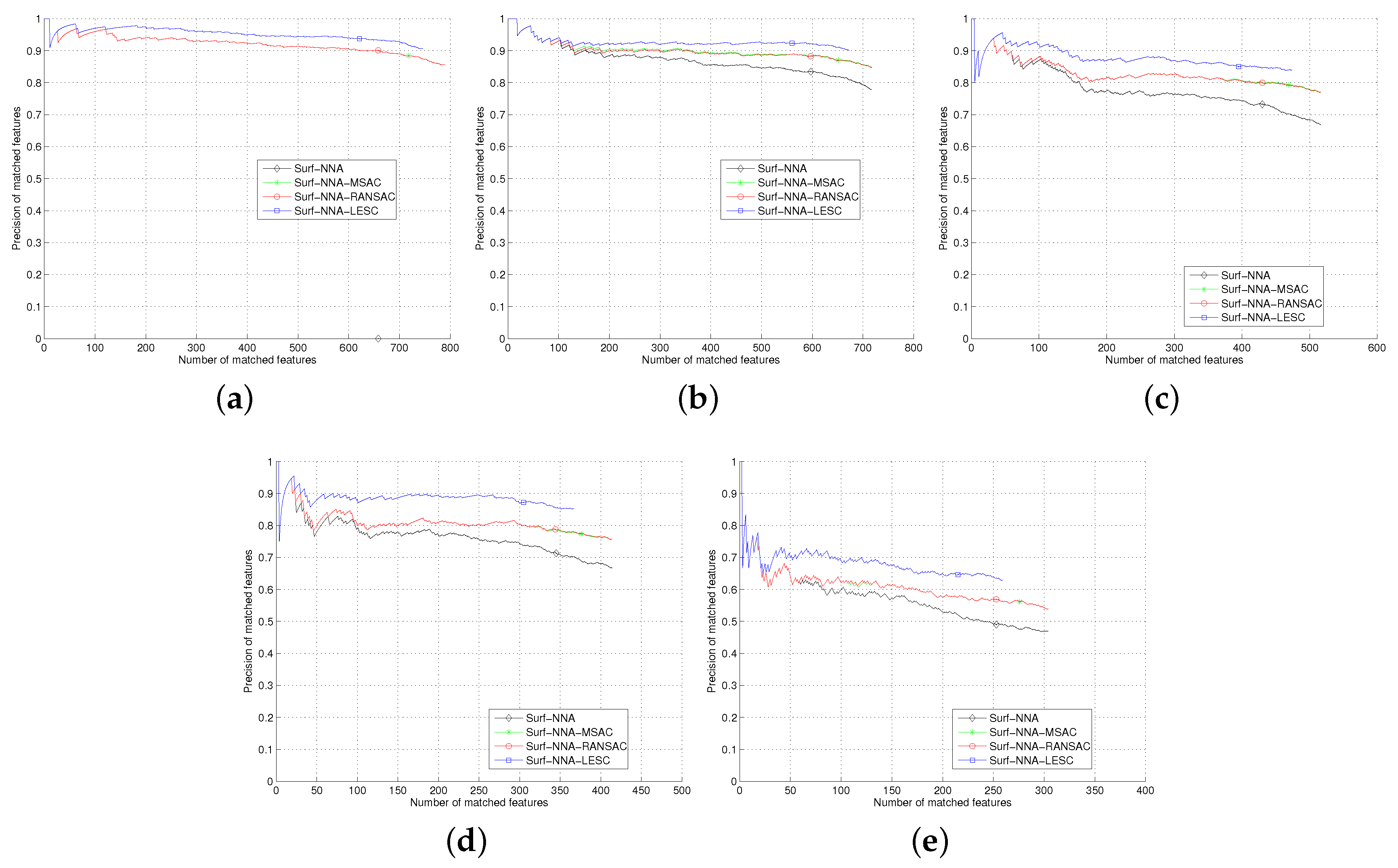
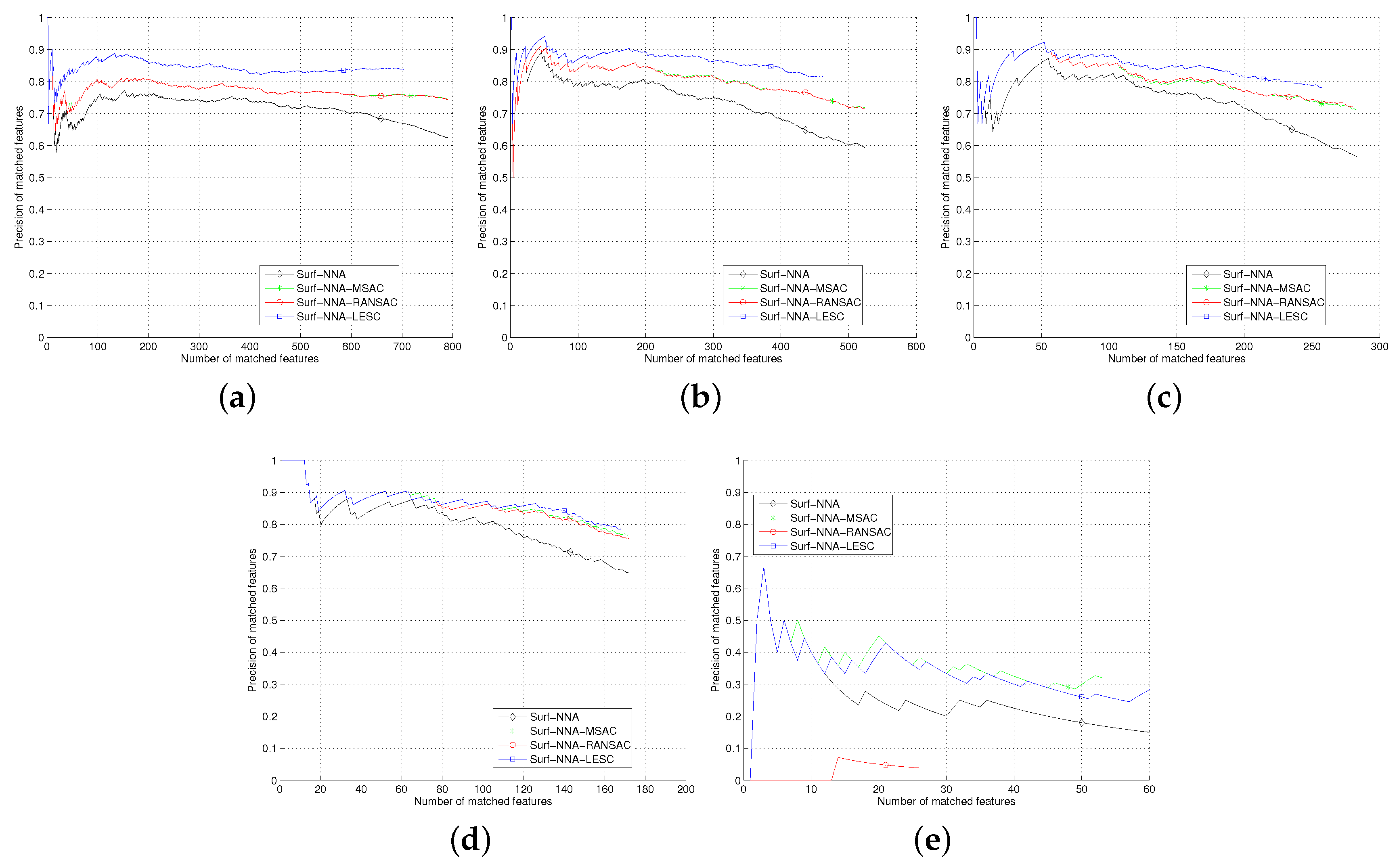
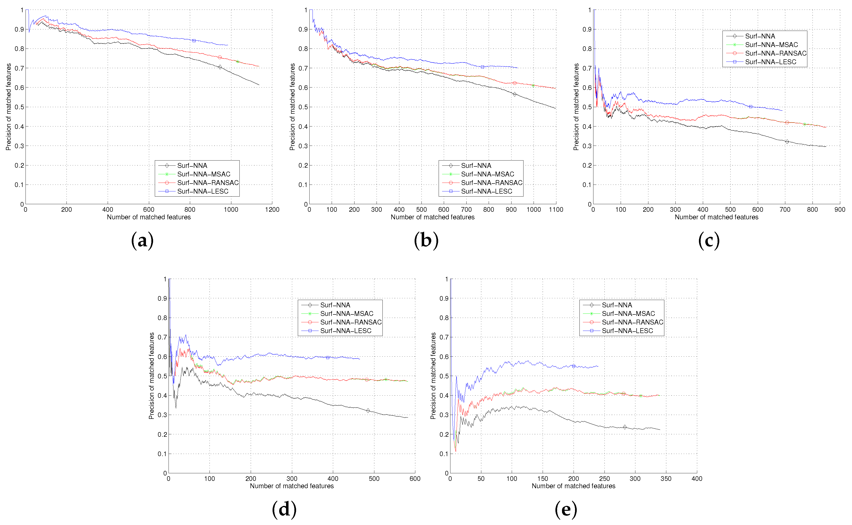
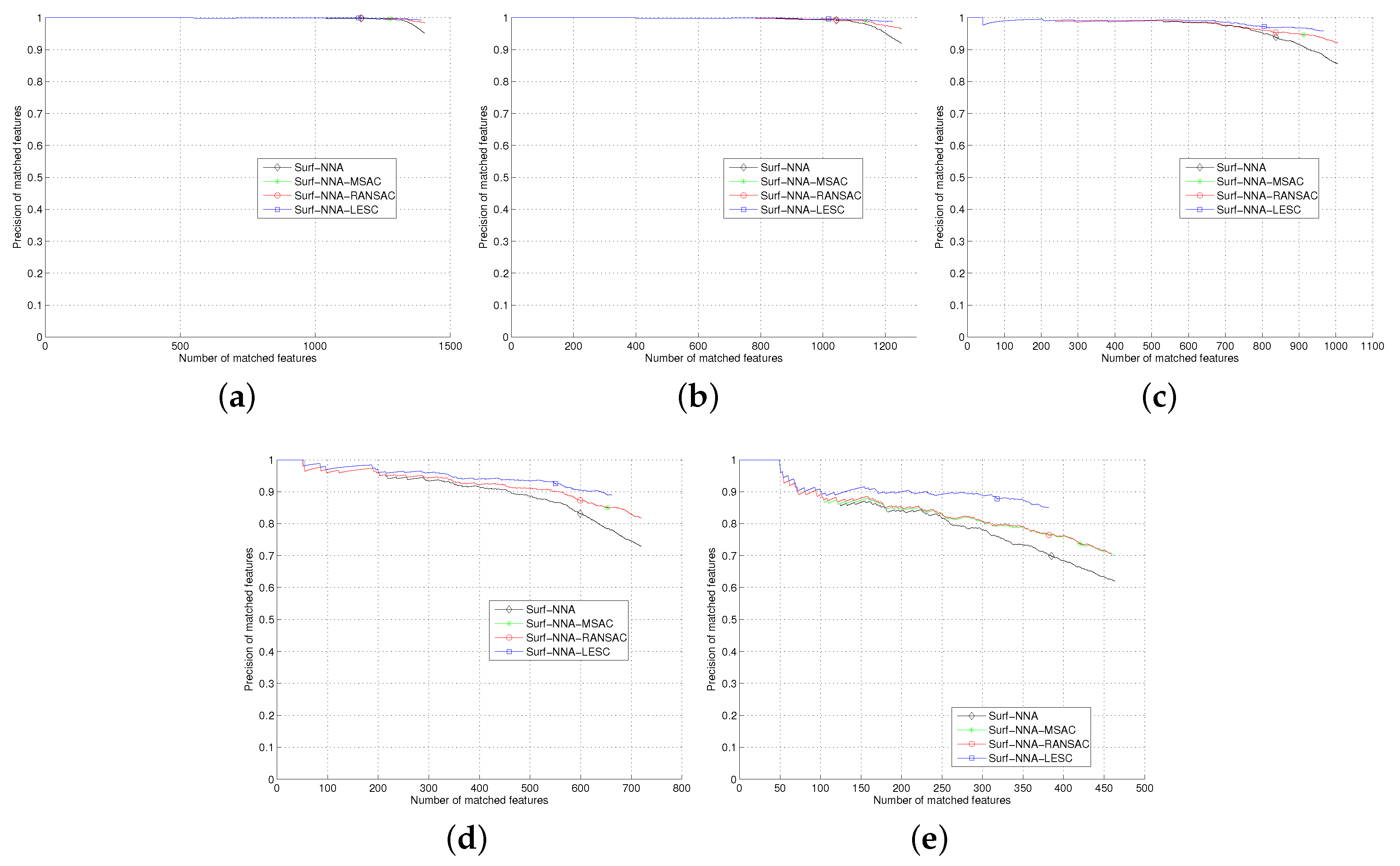
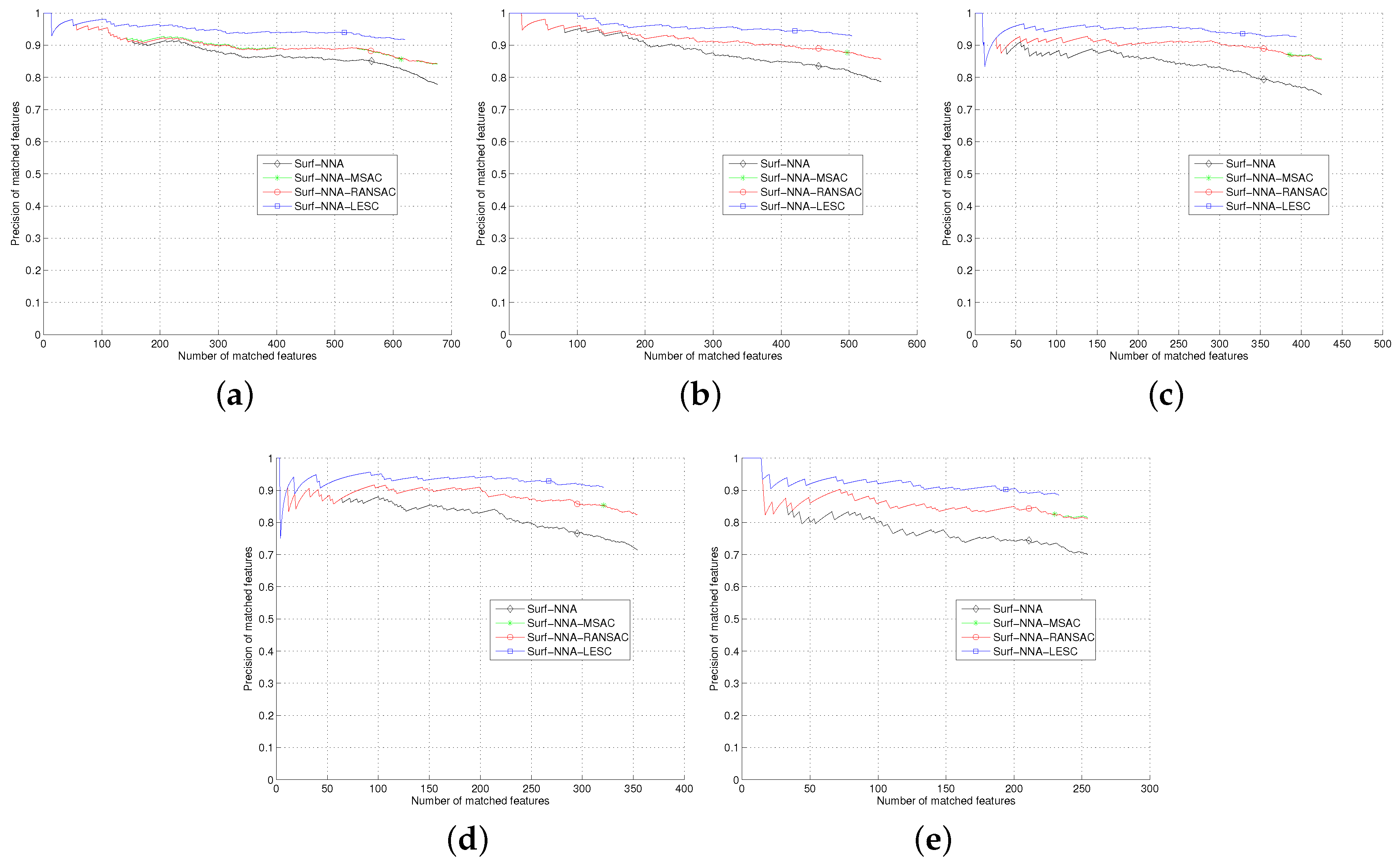
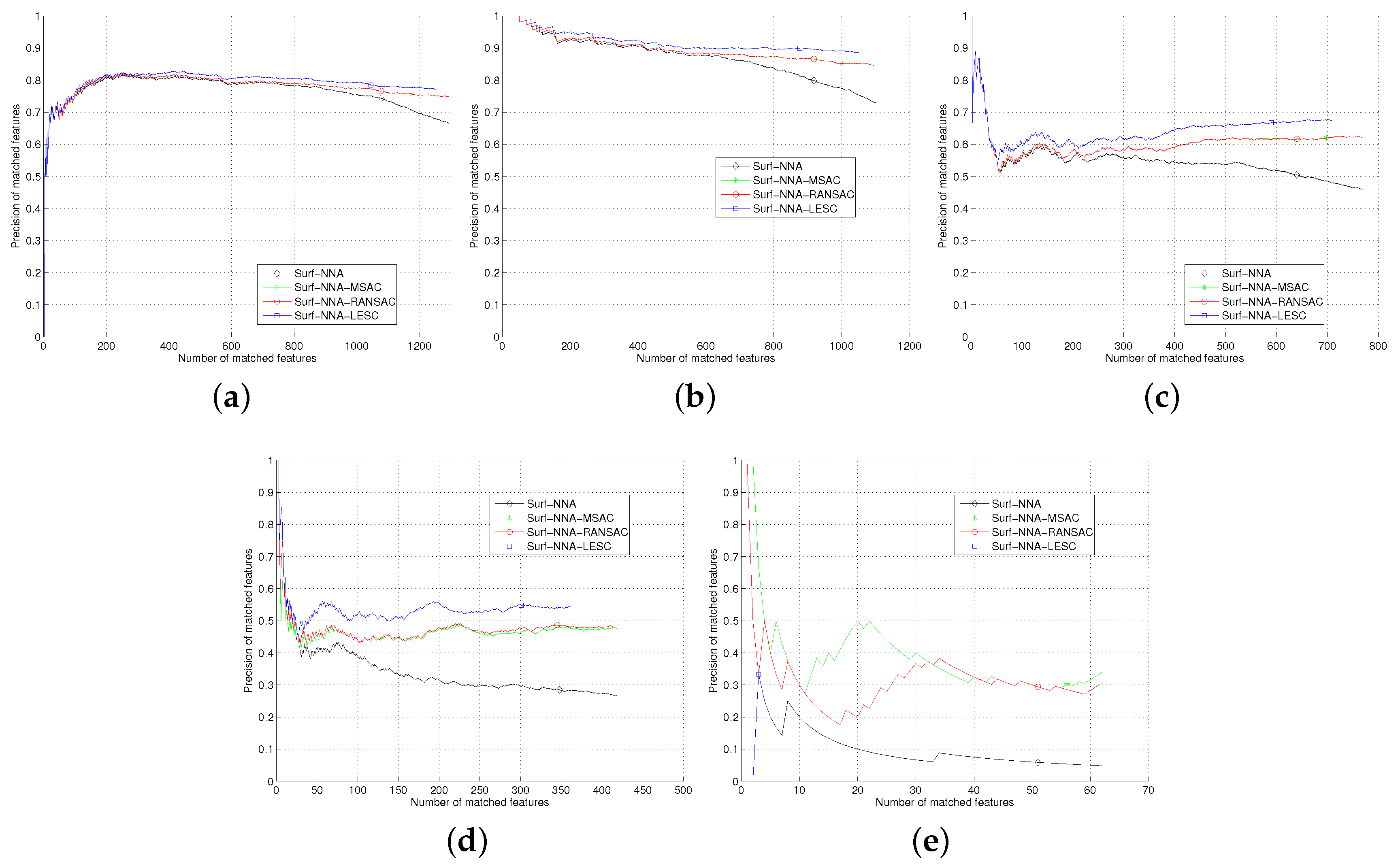
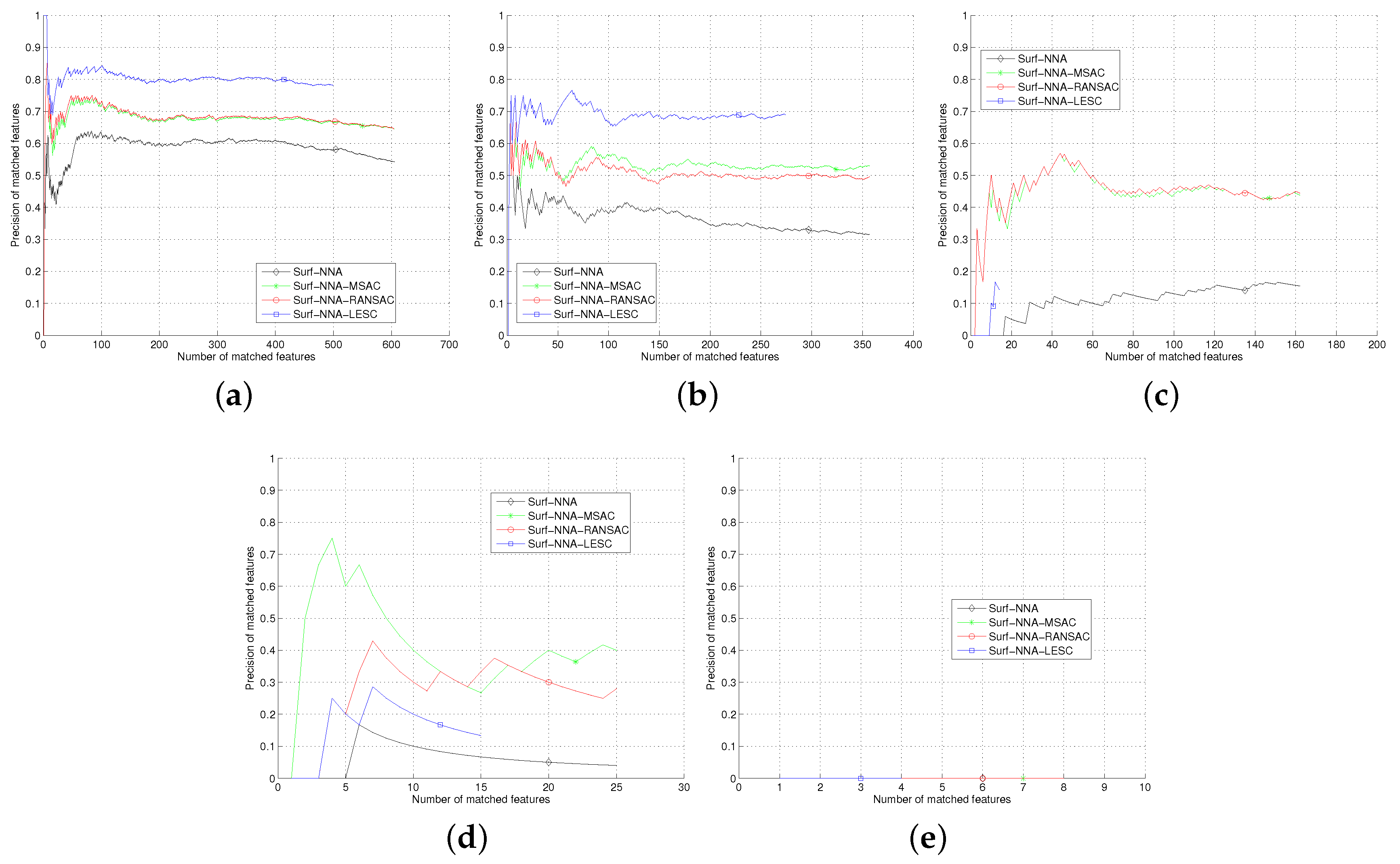
In the simulation of scale change for the textured scene (cf. Figure 1), LESC, RANSAC and MSAC have similar scores when there are more than 4 % inliers, whereas if the ratio of inliers is less than a small value, for example, 1.3 % in (e), RANSAC and MSAC find the consensus sets consisted of as many as 8 and 7 elements respectively but all these elements are not inliers. LESC gets advantages in four scale changes for the structured scene (cf. Figure 3) but is surpassed by MSAC under the situation of drastic change of scale. In the cases of blurred images, either structured scene or textured scene (cf. Figure 2 and Figure 4), as well as in the case of illumination change (cf. Figure 6), LESC noticeably overcomes RANSAC and MSAC in all fifteen comparisons. For JPEG compression, LESC also obtains higher performance than RANSAC and MSAC under increasing compression artefacts (cf. Figure 5). The most complex situation is viewpoint changes for either a textured scene or a structured scene. From 20 to 50 degrees changes of viewpoint for the textured scene (cf. Figure 7), LESC shows higher performance on precision than RANSAC and MSAC but at the viewpoint change of 60 degrees, LESC slumps to very low recall rate. A phenomenon for these viewpoint changes is that when the change degrees are greater than 30, the precision of these methods decreases severely. This phenomenon also appears under the situation of viewpoint change for the structured scene (cf. Figure 8), where at 60 degrees of the viewpoint change, although LESC, RANSAC and MSAC find some consensus sets but all data points in these sets are outliers. In the structured scene, LESC surpasses RANSAC and MSAC when the change of degrees is not greater than 30.
Since LESC produces generators by some statistics of increasing ranks, it dramatically lowers the cost for hypothesizing homographies and therefore in general matches features consuming less computation time than RANSAC and MSAC, which can be seen from Table 3, Table 4, Table 5, Table 6, Table 7, Table 8, Table 9 and Table 10. Moreover, in each test sequence the elapsed time of LESC are much more steady than the one of RANSAC and MSAC, which is a good property for some tasks sensitive to intervals of time.

6. Conclusions

We proposed the LESC method, which exploits LSE and order statistics to suppress noise in data and to diminish outliers for matching local features. Unlike other works employing the framework of RANSAC, our method generates hypothetical homographies determinatively according to the rank of the order statistics on the distance measurement and in effect roughly estimates the true homography and then iteratively refines the estimation to approximate it. LESC reaches higher precision-recall score than plain RANSAC in 31 scenes (and than MSAC in 30 scenes) out of total 40 test scenes. Because of the determinative sampling technique, in contrast to other methods of randomly selecting homography samples, LESC has advantages in its relatively stable cost of computation time for estimating the largest consensus set.

Author Contributions

Methodology, original draft and writing, Q.Z.; Supervision, B.S.; Data curation, H.X.

Funding

This research is supported by Guangdong Project of Science and Technology Development (2014B09091042) and Guangzhou Sci & Tech Innovation Committee (201707010068).

Acknowledgments

The authors appreciate Krystian Mikolajczyk for his test data set, and Macro Zuliani for his code of RANSAC, and Chris Evan for his code of OpenSURF.

Conflicts of Interest

The authors declare no conflict of interest.

References

  1. Fischler, M.A.; Bolles, R.C. Random Sample Consensus: A Paradigm for Model Fitting with Applications to Image Analysis and Automated Cartography. Commun. ACM 1981, 24, 381–395. [Google Scholar] [CrossRef]
  2. Torr, P.; Zisserman, A. MLESAC: A New Robust Estimator with Application to Estimating Image Geometry. Comput. Vis. Image Underst. 2000, 78, 138–156. [Google Scholar] [CrossRef] [Green Version]
  3. Konouchine, A.; Gaganov, V.; Veznevets, V. AMLESAC: A New Maximum Likelihood Robust Estimator. In Proceedings of the International Conference on Computer Graphics and Vision (GraphiCon), Novosibirsk Akademgorodok, Russia, 20–24 June 2005. [Google Scholar]
  4. Matas, J.; Chum, O. Randomized RANSAC with Td,d test. Image Vis. Comput. 2004, 22, 837–842. [Google Scholar] [CrossRef]
  5. Matas, J.; Chum, O. Randomized RANSAC with sequential probability ratio test. In Proceedings of the Tenth IEEE International Conference on Computer Vision (ICCV’05) Volume 1, Beijing, China, 17–20 October 2005; Volume 2, pp. 1727–1732. [Google Scholar] [CrossRef]
  6. Nister. Preemptive RANSAC for live structure and motion estimation. In Proceedings of the Ninth IEEE International Conference on Computer Vision, Nice, France, 13–16 October 2013; Volume 1, pp. 199–206. [Google Scholar] [CrossRef]
  7. Tordoff, B.J.; Murray, D.W. Guided-MLESAC: faster image transform estimation by using matching priors. IEEE Trans. Pattern Anal. Mach. Intell. 2005, 27, 1523–1535. [Google Scholar] [CrossRef] [Green Version]
  8. Chum, O.; Matas, J. Matching with PROSAC—Progressive sample consensus. In Proceedings of the 2005 IEEE Computer Society Conference on Computer Vision and Pattern Recognition (CVPR’05), San Diego, CA, USA, 20–26 June 2005; Volume 1, pp. 220–226. [Google Scholar] [CrossRef]
  9. Shi, C.; Wang, Y.; He, L. Feature matching using sequential evaluation on sample consensus. In Proceedings of the 2017 International Conference on Security, Pattern Analysis, and Cybernetics (SPAC), Shenzhen, China, 15–17 December 2017; pp. 302–306. [Google Scholar] [CrossRef]
  10. Raguram, R.; Frahm, J.M.; Pollefeys, M. Exploiting uncertainty in random sample consensus. In Proceedings of the 2009 IEEE 12th International Conference on Computer Vision, Kyoto, Japan, 29 September–2 October 2009; pp. 2074–2081. [Google Scholar] [CrossRef]
  11. Bhattacharya, P.; Gavrilova, M. DT-RANSAC: A Delaunay Triangulation Based Scheme for Improved RANSAC Feature Matching. In Transactions on Computational Science XX: Special Issue on Voronoi Diagrams and Their Applications; Gavrilova, M.L., Tan, C.J.K., Kalantari, B., Eds.; Springer: Berlin/Heidelberg, Germany, 2013; pp. 5–21. [Google Scholar]
  12. Wang, Y.; Zheng, J.; Xu, Q.Z.; Li, B.; Hu, H.M. An improved RANSAC based on the scale variation homogeneity. J. Vis. Commun. Image Represent. 2016, 40, 751–764. [Google Scholar] [CrossRef] [Green Version]
  13. Fotouhi, M.; Hekmatian, H.; Kashani-Nezhad, M.A.; Kasaei, S. SC-RANSAC: Spatial consistency on RANSAC. Multimed. Tools Appl. 2018. [Google Scholar] [CrossRef]
  14. İmre, E.; Hilton, A. Order Statistics of RANSAC and Their Practical Application. Int. J. Comput. Vis. 2015, 111, 276–297. [Google Scholar] [CrossRef]
  15. Chum, O.; Matas, J.; Kittler, J. Locally Optimized RANSAC. In Pattern Recognition; Michaelis, B., Krell, G., Eds.; Springer: Berlin/Heidelberg, Germay, 2003; pp. 236–243. [Google Scholar]
  16. Lowe, D.G. Object recognition from local scale-invariant features. In Proceedings of the Seventh IEEE International Conference on Computer Vision, Kerkyra, Greece, 20–27 September 1999; Volume 2, pp. 1150–1157. [Google Scholar] [CrossRef]
  17. Lowe, D.G. Distinctive Image Features from Scale-Invariant Keypoints. Int. J. Comput. Vis. 2004, 60, 91–110. [Google Scholar] [CrossRef]
  18. Bay, H.; Tuytelaars, T.; Van Gool, L. SURF: Speeded Up Robust Features. In Proceedings of the European Conference on Computer Vision, Graz, Austria, 7–13 May 2006; pp. 404–417. [Google Scholar]
  19. Bay, H.; Ess, A.; Tuytelaars, T.; Gool, L.V. Speeded-Up Robust Features (SURF). Comput. Vis. Image Underst. 2008, 110, 346–359. [Google Scholar] [CrossRef]
  20. Mikolajczyk, K.; Tuytelaars, T.; Schmid, C.; Zisserman, A.; Matas, J.; Schaffalitzky, F.; Kadir, T.; Gool, L.V. A Comparison of Affine Region Detectors. Int. J. Comput. Vis. 2005, 65, 43–72. [Google Scholar] [CrossRef]
Figure 1. Scale change for the textured scene by the Bark sequence. From (a) to (e) the degree of change ascends.
Information 10 00275 g001
Figure 2. Blur for the structured scene by the Bikes sequence. From (a) to (e) the degree of change ascends.
Information 10 00275 g002
Figure 3. Scale change for the structured scene by the Boat sequence. From (a) to (e) the degree of change ascends.
Information 10 00275 g003
Figure 4. Blur for the textured scene by the Trees sequence. From (a) to (e) the degree of change ascends.
Information 10 00275 g004
Figure 5. JPEG compression by the UBC sequence. From (a) to (e) the degree of change ascends.
Information 10 00275 g005
Figure 6. Illumination change by the Leuven sequence. From (a) to (e) the degree of change ascends.
Information 10 00275 g006
Figure 7. Viewpoint change for the textured scene by the Wall sequence. From (a) to (e) the degree of change ascends.
Information 10 00275 g007
Figure 8. Viewpoint change for the structured scene by the Graffiti sequence. From (a) to (e) the degree of change ascends.
Information 10 00275 g008
Table 1. Main Parameters in RANSAC and MSAC.
χ 2 probability threshold for inliers 1 e 4
False alarm rate e 6
Maximum number of iterations100,000
Minimum number of iterations1
The σ of assumed Gaussian noise1
Table 2. An example of the influence of R in Algorithm 1 to the Elapsed time and the number of recalls.
Settings of R00.010.020.050.1
Elapsed time (seconds) 6.392 0.466 0.186 0.060 0.029
Number of recalls621620619615612
Table 3. The computation time (in seconds) of LESC, RANSAC and MSAC respectively on the Bark sequence using the 1st image versus the rest of images.
Method1 vs. 21 vs. 31 vs. 41 vs. 51 vs. 6
LESC 0.124 0.238 0.231 0.172 0.074
RANSAC 9.127 195.041 211.282 210.633 213.429
MSAC 9.456 206.953 212.522 210.419 213.408
Table 4. The computation time (in seconds) of LESC, RANSAC and MSAC respectively on the Boat sequence using the 1st image versus the rest of images.
Method1 vs. 21 vs. 31 vs. 41 vs. 51 vs. 6
LESC 0.431 0.478 0.368 0.100 0.135
RANSAC 2.070 6.874 12.967 85.802 170.648
MSAC 2.270 6.142 15.308 102.652 173.758
Table 5. The computation time (in seconds) of LESC, RANSAC and MSAC respectively on the Bikes sequence using the 1st image versus the rest of images.
Method1 vs. 21 vs. 31 vs. 41 vs. 51 vs. 6
LESC 0.256 0.120 0.288 0.311 0.073
RANSAC 0.278 0.255 0.363 0.348 0.327
MSAC 0.270 0.265 0.368 0.336 0.299
Table 6. The computation time (in seconds) of LESC, RANSAC and MSAC respectively on the Trees sequence using the 1st image versus the rest of images.
Method1 vs. 21 vs. 31 vs. 41 vs. 51 vs. 6
LESC 0.226 0.487 0.293 0.592 0.207
RANSAC 4.739 5.010 15.057 72.853 277.446
MSAC 4.331 5.319 14.351 81.059 270.460
Table 7. The computation time (in seconds) of LESC, RANSAC and MSAC respectively on the UBC sequence using the 1st image versus the rest of images.
Method1 vs. 21 vs. 31 vs. 41 vs. 51 vs. 6
LESC 0.335 0.196 0.186 0.567 0.276
RANSAC 0.225 0.211 0.383 0.887 4.828
MSAC 0.227 0.353 0.320 1.003 4.858
Table 8. The computation time (in seconds) of LESC, RANSAC and MSAC respectively on the Leuven sequence using the 1st image versus the rest of images.
Method1 vs. 21 vs. 31 vs. 41 vs. 51 vs. 6
LESC 0.466 0.259 0.329 0.260 0.094
RANSAC 0.206 0.230 0.239 0.243 0.388
MSAC 0.230 0.220 0.287 0.225 0.323
Table 9. The computation time (in seconds) of LESC, RANSAC and MSAC respectively on the Wall sequence using the 1st image versus the rest of images.
Method1 vs. 21 vs. 31 vs. 41 vs. 51 vs. 6
LESC 0.168 0.459 0.186 0.277 0.061
RANSAC 1.052 1.848 8.183 98.532 286.434
MSAC 0.934 2.046 8.207 92.270 290.465
Table 10. The computation time (in seconds) of LESC, RANSAC and MSAC respectively on the Graffiti sequence using the 1st image versus the rest of images.
Method1 vs. 21 vs. 31 vs. 41 vs. 51 vs. 6
LESC 0.738 0.188 0.149 0.186 0.049
RANSAC 2.511 19.248 217.795 230.480 230.250
MSAC 2.559 27.735 219.145 232.490 230.998