Enhanced Grid-Based Visual Analysis of Retinal Layer Thickness with Optical Coherence Tomography ^†

Abstract

Optical coherence tomography enables high-resolution 3D imaging of retinal layers in the human eye. The thickness of the layers is commonly assessed to understand a variety of retinal and systemic disorders. Yet, the thickness data are complex and currently need to be considerably reduced prior to further processing and analysis. This leads to a loss of information on localized variations in thickness, which is important for early detection of certain retinal diseases. We propose an enhanced grid-based reduction and exploration of retinal thickness data. Alternative grids are computed, their representation quality is rated, and best fitting grids for given thickness data are suggested. Selected grids are then visualized, adapted, and compared at different levels of granularity. A visual analysis tool bundles all computational, visual, and interactive means in a flexible user interface. We demonstrate the utility of our tool in a complementary analysis procedure, which eases the evaluation of ophthalmic study data. Ophthalmologists successfully applied our solution to study localized variations in thickness of retinal layers in patients with diabetes mellitus.

1. Introduction

Optical coherence tomography (OCT) [1] is a widely-used noninvasive technique to capture high-resolution 3D images of retinal substructures. Ophthalmologists analyze the resulting data to understand a variety of retinal and systemic disorders [2]. This includes common eye diseases, e.g., age-related macular degeneration [3], diabetic retinopathy [4], or glaucoma [5]; other pathologies with ocular signs, e.g., multiple sclerosis [6]; and retinal vascular disorders [7]. Particularly, the thickness of segmented retinal layers is used to assess the condition of the retina. However, derived thickness data are complex, as one thickness value is computed for every single point of each retinal layer. On the one hand, this enables a spatially precise judgment of the layers. On the other hand, the large amounts of thickness values are difficult to deal with, and a summary of thickness changes in larger retinal areas is missing. Hence, ophthalmologists rely on considerable data reduction prior to further processing and analysis of the data.

Established reduction methods for retinal thickness data are based on retinal grids. These grids are used to spatially divide the retina into few large regions and to derive aggregated thickness measures for each region. This helps to get a quick overview of the layers’ thickness in anatomically predefined areas. Moreover, it drastically reduces the amount of information to be analyzed, particularly in larger studies with dozens or hundreds of OCT datasets. Yet, due to the spatial aggregation, information loss may occur. This is because small and localized variations in thickness are not always reasonably represented via aggregated values of large regions. Capturing such information is however mandatory for detecting early signs of certain diseases or investigating progressions.

We aim at supporting ophthalmologists in their grid-based visual analysis of retinal layer thickness. We propose an enhanced data reduction scheme together with a visual analysis tool for the exploration of alternative grids. Our approach helps to strike a balance between obtaining a compact grid representation of thickness data and being able to capture more relevant information of retinal layers. Our contributions are:

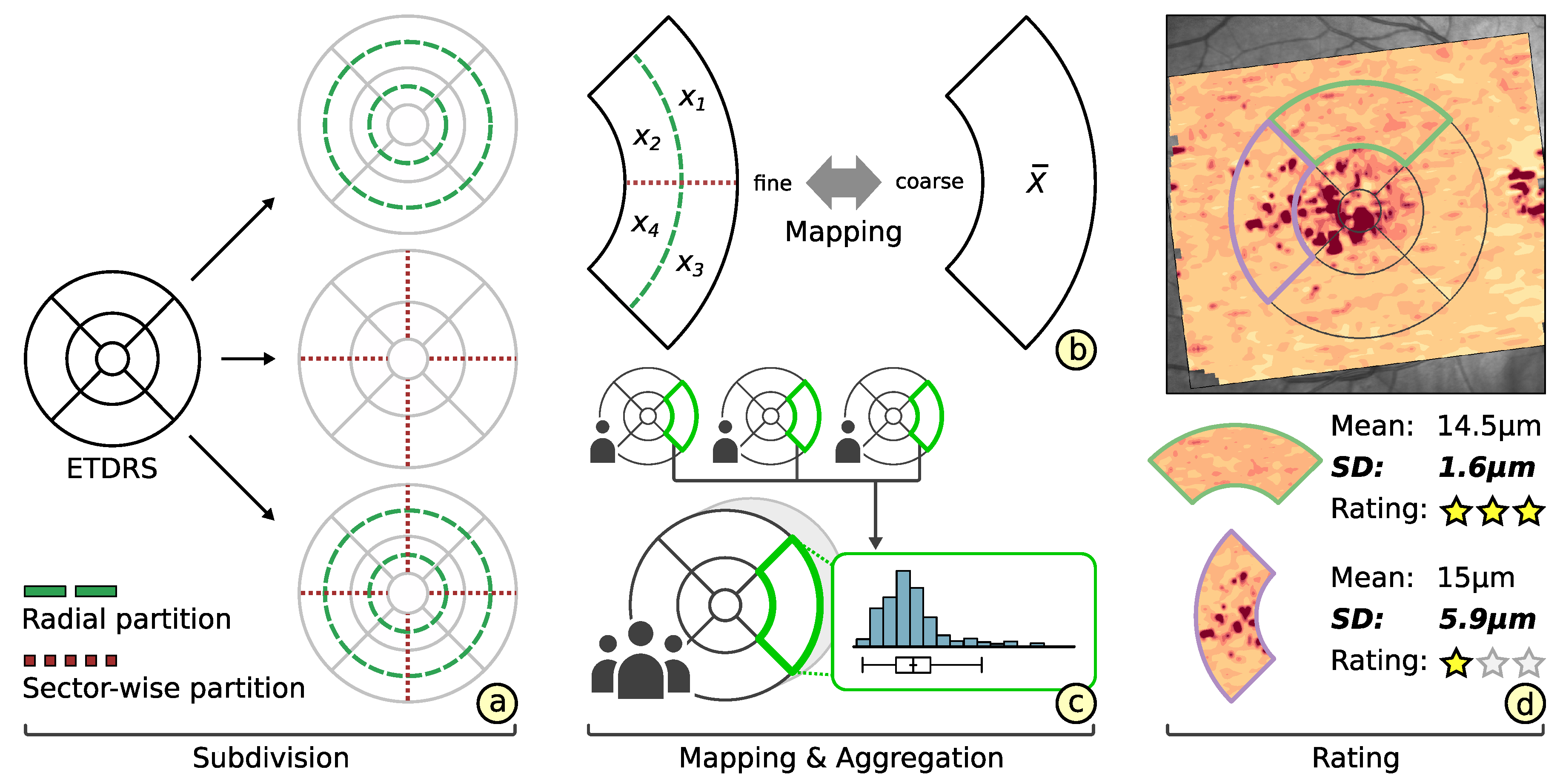
• Enhanced grid design: We propose an adaptive grid-based reduction of retinal thickness data. New grid layouts are derived by radial and sector-wise subdivision of well-established grids. The representation quality of alternative grids is rated and best options are suggested to the user.
• Grid-based visual analysis: We develop a flexible visual analysis tool for grid-based data exploration. Grids are interactively refined, compared to other grids, and cell-related details are shown on demand. A complementary procedure eases the analysis of ophthalmic study data.
• Evaluation of ophthalmic studies: We apply our tool to investigate localized variations in retinal layer thickness in two cross-sectional studies with patients suffering from diabetes mellitus. The main findings are summarized and compared to results of current analysis procedures.

This paper constitutes an extension of our previous work [8]. We continue our collaboration with ophthalmologists, which allows us to define design requirements and to test our solutions in comparison with their current analysis practices. We integrate our enhanced grid design and exploration in a flexible visual analysis tool and describe how an associated analysis procedure helped ophthalmologists to evaluate data of two ophthalmic studies. We summarize gathered feedback, broaden the discussion of results, and exemplify other application scenarios in ophthalmology.

After describing the medical background, related work, and current analysis procedures in Section 2, we present our enhanced grid design in Section 3. Based on new grid layouts, we introduce our interactive exploration of retinal thickness data in Section 4. We then propose a matched visual analysis tool and analytic process in Section 5, and apply them to ophthalmic study data in Section 6. Lastly, we summarize our work and discuss future research directions in Section 7.

2. Background

Our work is motivated and driven by advances in the detection of retinal diseases [9]. Particularly, the dynamic development of OCT technology with respect to image quality offers a unique possibility of differentiating and precisely measuring retinal substructures [10,11,12], close to an in vivo ‘optical biopsy’ of the retina [13]. Modern OCT devices enable high-resolution imaging of biological tissue in the micrometer range with an approximate axial and lateral resolution of 2 $\mathsf{\mu }$$\mathrm{m}$ [14] or even almost submicron lateral resolution [15]. The commercially available system used in our work (Spectralis^® HRA + OCT, OCT2 Module, Heidelberg Engineering GmbH, Heidelberg, Germany) is based on frequency domain optical coherence technology (also called spectral-domain or Fourier-domain OCT). It captures cross-sectional depth images (B-scans) of the retina at high speed (axial scan rate of 85 kHz) with an axial and lateral image resolution of $3.5$ $\mathsf{\mu }$$\mathrm{m}$/pixel and 6 to 11 $\mathsf{\mu }$$\mathrm{m}$/pixel, respectively. Typically, multiple B-scans are combined to obtain volumetric 3D images and further processed, including noise reduction [16] and segmentation of retinal layers [17]. This provides a straightforward method of assessing even subtle retinal changes and accurately monitoring the progression of a disease. Consequently, OCT examinations are now a standard of care in clinical practice and an essential tool in ophthalmic research [18]. Based on the data, ophthalmologists aim at performing both

• patient-specific assessments of the retinal condition of individuals and
• group-specific evaluations of experimental and prospective studies.

In this context, they often need to compare multiple intraindividual datasets, e.g., follow-up examinations of a single patient, and interindividual datasets, e.g., examinations of patients in relation to normative data of controls. Yet, the data analysis can be complex and the available analysis methods differ between existing software tools. In this regard, our work is related to the visual analysis of retinal OCT data in general, and to the representation of retinal layer thickness via grids in particular.

2.1. Visual Analysis of OCT Data

Current analysis procedures are based on a combination of commercial OCT software, noncommercial OCT software, and general-purpose analysis software. Segmentation of retinal layers and measurement of layer thickness are supported by both commercial software and noncommercial software [19,20,21]. Commercial OCT software is commonly distributed by OCT device manufactures. Besides commercial software, few approaches for visually analyzing retinal OCT data exist. Examples are the research-oriented Iowa Reference Algorithms [19], the open source software ImageJ [22] and its application to OCT data [23], a ray-traced 3D visualization of OCT data [24], machine learning-based systems for visual diagnosis and referral support [25], and a recent visual analysis software based on multiple coordinated views [26]. These software tools are typically applied in ophthalmic research rather than in clinical practice. All available software packages support at least one of three fundamental presentation methods: cross-sectional views, 3D views, and top-down views.

Cross-sectional views show individual B-scans of volumetric OCT data together with overlaid profiles of segmented retinal layers. This allows to view details but flipping through the images is time-consuming, as OCT datasets can consist of hundreds of B-scans. 3D views show an entire OCT dataset as a 3D volume rendered tomogram. This provides an overview of the data but combined 3D visualizations of the tomogram and the layers are only provided by few tools, e.g., the work by the authors of [26]. Top-down views show a fundus image of the interior surface of the eye around the OCT acquisition area together with superimposed retinal layers. This facilitates a layer-centric analysis of the data and helps to link the layers to retinal areas in the fundus image. In general, cross-sectional views and 3D views are mainly used for the visual analysis of individual datasets, whereas top-down views are also applied to anatomically localize and compare areas under investigation in multiple OCT datasets. In this regard, top-down views are most relevant to our work.

Instead of showing the raw OCT data, top-down views typically represent retinal layers via their derived layer thickness. The layer thickness is displayed either via thickness maps or via spatially aggregated thickness grids. This helps to reveal retinal changes, which may be difficult to identify by visualizing the raw OCT data alone. While recently there has been progress in the comparative visualization of thickness maps in OCT data [26,27], thickness grids are still predominantly used in most ophthalmic applications. One reason for this is that thickness maps, albeit being spatially precise, can be unnecessarily complex compared to simpler grids in certain situations and they tend to be more difficult to analyze with respect to anatomically distinct retinal areas. On the other hand, the design of thickness grids has been hardly investigated in earlier work, despite the continuous development of OCT technology and analysis methods. In fact, in ophthalmic research, only few standardized grids have been employed for data analysis and study results are mostly shown as statistical plots or numbers in a table without spatial context. On this account, we focus on the grid-based exploration of retinal thickness data. Our main objective is to support an information-aware data reduction that preserves relevant details while summarizing remaining parts to a manageable amount.

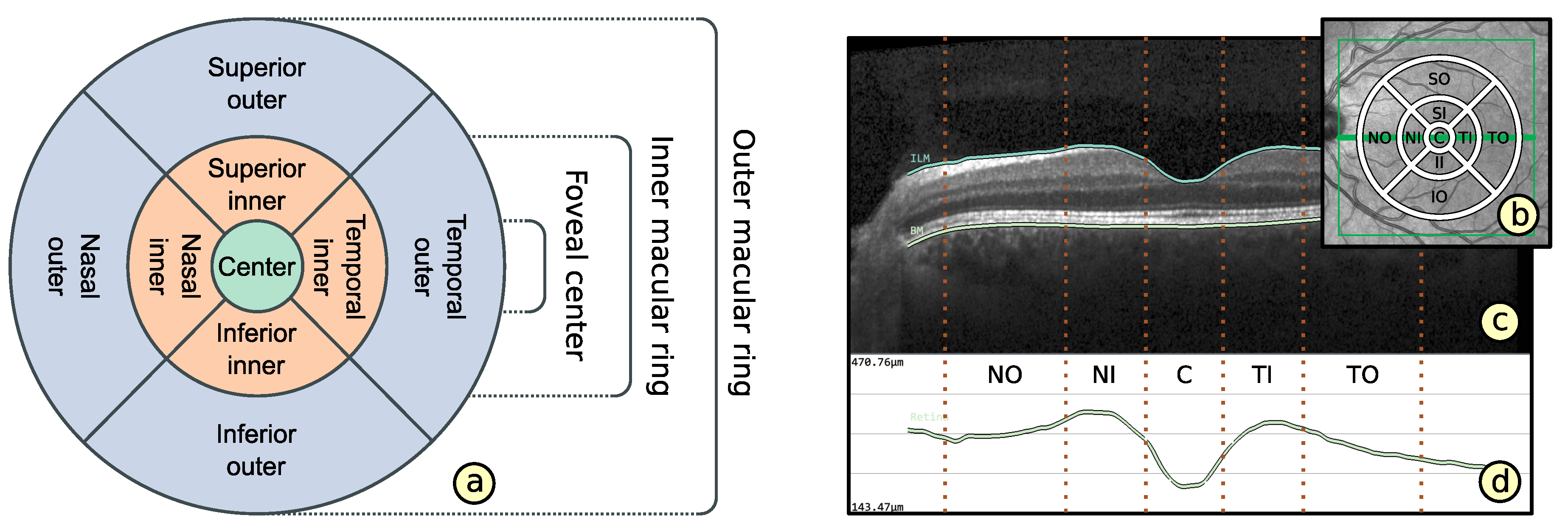
2.2. Representation of Retinal Layer Thickness via ETDRS Grids

The most common grid type for retinal thickness data was established by the Early Treatment Diabetic Retinopathy Study (ETDRS) [28]. The ETDRS grid cells divide the retina into nine large regions defined by three rings: a central foveal ring with 1mm diameter, an inner macular ring (pericentral) with 3mm diameter, and an outer macular ring (peripheral) with 6mm diameter. The inner and outer rings are divided into four quadrants: nasal, temporal, superior, and inferior. Figure 1 shows the resulting cell layout. For each grid cell and retinal layer, one aggregated thickness measurement, e.g., the arithmetic mean, is stored. Figure 2 illustrates the generation of the grid data. ETDRS grids have been widely applied for various purposes in ophthalmic research, including investigations of early retinal changes for a variety of diseases, e.g., diabetes mellitus [29] and glaucoma [30]. Although other grid types exist, they have been mostly designed for special applications, e.g., rectangular grids for asymmetry analysis of retinal thickness in glaucoma diagnosis [31].

An advantage of ETDRS grids is their compact representation of complex thickness data. This allows a quick overview of thickness changes in predefined retinal areas. The layout of ETDRS grid cells also accounts for natural differences in the shape of the retina. It enables the localization of important areas of the macula near the center of the retina and the assessment of thickness data with respect to each anatomically distinct location. Moreover, the fixed data reduction eases the evaluation and comparison of multiple datasets, even from different studies.

The main problem with ETDRS grids is, however, that they represent aggregated thickness data (Figure 3). Due to the considerable spatial data reduction, localized variations in thickness are not accurately captured via a single aggregated thickness value per grid cell. This is the case for both small variations in thickness within a grid cell and variations divided by the boundary of two or more grid cells (Figure 3c,d). Moreover, when evaluating deviations between thickness data of several datasets, aggregation artifacts may lead to false normal findings. The reason for this is that localized positive and negative deviations within a grid cell can get nullified during data reduction (Figure 3h,i). Detecting such information is vital for the identification of early retinal changes of certain diseases.

3. Grid Design

ETDRS grids are well-established and widely-used. We aim at designing alternative grids that combine the advantages of ETDRS grids with the possibility to capture more relevant information. To this end, we identified grid-related design requirements, devised a new subdivision scheme that allows to compare grid layouts, and developed a method to rate the representation quality of grids.

3.1. Grid-Related Requirements

The grid-related design requirements reflect the ophthalmologists’ needs with regard to processing and analyzing retinal thickness data. We derived the following list by talking with ophthalmologists about current limitations and the way they utilize existing grids to analyze retinal thickness data.

• Layout based on ETDRS grid ($G{R}_1$): The basic layout of alternative grids should correspond to the ETDRS grid. This is to maintain the ability to localize anatomically important areas of the macula near the center of the retina.
• Comparability of grid layouts ($G{R}_2$): Alternative grid layouts should be comparable to both the basic ETDRS grid and other alternative grids. This is to ensure that analysis results from multiple datasets with different grids are relatable.
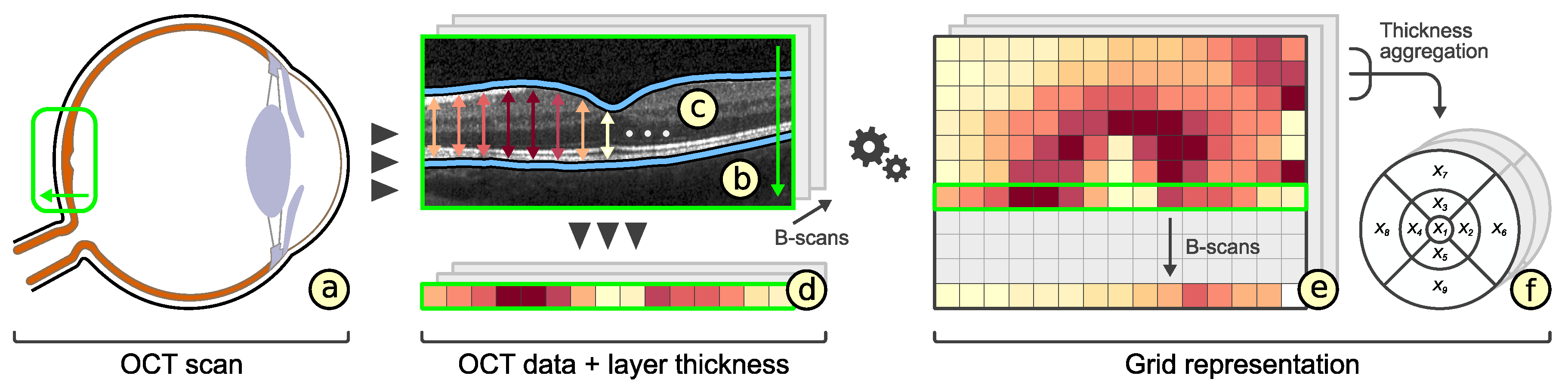
• Compact data representation ($G{R}_3$): The number of grid cells should be small and the content of a grid cell should be represented by mainly one descriptive value. Nevertheless, an appropriate representation of thickness data has to be facilitated.

3.2. Subdivision of Grids

Based on the ophthalmologists’ demands, we design alternative grids that meet requirements $G{R}_1$ and $G{R}_3$. Taking the ETDRS grid as a basis, we employ a radial or sector-wise partitioning strategy for ETDRS grid cells. This allows us to obtain alternative grids that represent the underlying thickness data at different levels of granularity. Figure 4a exemplifies both partitioning strategies.

Radial partitions add rings to a grid. The resulting grid cells enable a more fine-grained analysis of areas with respect to the distance from the foveal center. For example, retinal layer thickness of macular rings can be investigated in-depth via secondary inner or outer ring cells. Sector-wise partitions add separating lines at certain angles to a grid. The generated grid cells facilitate a direction-centric analysis of areas with respect to the foveal center. For example, by adding further directional cells, the thickness of areas facing nasally may be evaluated in greater detail. Radial and sector-wise partitions can be combined to obtain fine grids that support analyses with focus on both properties.

To restrict the number of all possible combinations of subdivisions, we start by equally dividing grid cells and increase the number of radii or sectors in power of two steps. By dividing grid cells in half in each subdivision pass, the amount of information stored in a subdivided grid is increased in constant steps. The resulting set of grids can then be refined interactively. Just like standard ETDRS grids, we represent the content of each grid cell via one aggregated thickness measurement. Optionally, summary statistics, e.g., mean, percentiles, and standard deviation, are stored per cell to provide further information on the distribution of the underlying thickness data.

Subdividing the standard ETDRS grid helps ophthalmologists to familiarize themselves with the layout of derived grids. Added cells are easily associated with anatomically distinct retinal areas. This increases the acceptance of alternative grids.

3.3. Comparability of Grids

Ophthalmologists are often interested in relating grid-based analysis results from multiple datasets (cf. $G{R}_2$). Each dataset of individual patients may be best represented by another grid with a different layout. To ensure the comparability of the grids, we support mapping a fine grid to a coarse grid and vice versa. This is possible as in our design a fine grid is basically a subdivided version of a coarse grid. Figure 4b illustrates both mapping strategies. In addition, grids of a patient group may have to be compared to grids of another patient group or of a control group. On this account, we allow to compile multiple source grids of a group into a single aggregated grid. The aggregated grid cells can then be mapped and assigned values can be directly related. Figure 4c shows the aggregation of grids.

Mapping a fine grid to a coarse grid entails that subdivided cells have to be merged together to the granularity level of coarser cells. The values of merged cells are determined by aggregating the values of subdivided cells, e.g., by computing and storing their arithmetic mean. A prominent example for this mapping strategy is the backtracking of alternative grids to the standard ETDRS grid. This allows to compare new analysis results obtained via our grid design to results based on the ETDRS grid in previous ophthalmic studies. Another example is to pick the coarsest subdivision grid from a set of alternatives and to map the other grids to that reference. This is necessary if the thickness data are no longer available, and thus merging finer cells is the only option.

Mapping a coarse grid to a fine grid involves that coarse cells are subdivided to the granularity level of fine cells. The values of the subdivided cells are then assigned either by recomputing them based on the underlying thickness data or simply by copying the values of corresponding coarser cells. A precondition for the second case is that the coarse grid is a good data representation, and consequently a subdivided version of that grid represents the data equally well, i.e., it just consists of more grid cells. An advantage of this mapping strategy is that no details stored via finer grid cells are lost during a comparison. This is important if a fine grid representing a patient with abnormal localized variations in thickness has to be compared to a coarser grid representing normative data of healthy controls, which commonly show less variations in thickness.

Compiling an aggregated grid implies that multiple source grids are transformed into a single grid representation. First, a layout for the aggregated grid is determined and then the source grids are mapped to that common layout. The aggregated grid represents the source grids via one descriptive value per cell, e.g., the arithmetic mean of corresponding source cell values. In addition, summary statistics of source values may be stored per aggregated grid cell. To analyze two or more aggregated grids, they are mapped using one of the above strategies and related based on corresponding cell values. This way, a grid of a single patient or an aggregated grid of a patient group can be compared to an aggregated grid of a control group.

3.4. Rating of Grids

Generally, there is no single grid layout that represents all spatial distributions of thickness data equally well. Based on our partitioning strategies, we instead get a set of readily available alternative grids. In order to suggest which of these grids actually corresponds to the given data, we developed a rating procedure that measures the representation quality of individual grids. Our rating of grids addresses the second aspect of grid-related requirement $G{R}_3$. Figure 4d exemplifies the grid rating.

We compute the representation quality of a grid by measuring the homogeneity of thickness values within each cell. This is based on the assumption that a cell with high homogeneity covers values that are more or less equal, whereas a cell with low homogeneity encloses strongly varying values. Thus, a cell value with high homogeneity matches the data, whereas a cell value with low homogeneity indicated information loss. Consequently, a grid consisting of homogeneous cells corresponds to a good representation of the thickness data and vice versa.

One possible measure to quantify the amount of variation or homogeneity of a set of thickness values is the standard deviation. With this simple measure, we obtain the overall rating of a grid via the weighted arithmetic mean of the standard deviations of all grid cells.

$$\overline{x}=\frac{{\sum }_{i=1}^n{w}_i{x}_i}{{\sum }_{i=1}^n{w}_i}$$

In this equation, $\overline{x}$ represents the final rating of the grid, n denotes the number of grid cells, $x_i$ is the standard deviation of a cell, and $w_i$ is the weight for that cell given by the normalized amount of enclosed data points (equal to the size of the cell). Based on the final ratings, we compute a ranking for a set of alternative grids and suggest a best fit for thickness data of one retinal layer while considering secondary constraints by ophthalmologists. Such constraints are a specified maximum number of allowed grid cells or a preference for either radial or sector-wise subdivisions. This promotes a more patient-specific analysis in contrast to generalizing all given thickness data to just the ETDRS grid representation. Likewise, the rating and ranking can be adapted to support a group-specific assessment of grids. The procedures allow to determine one best fitting grid for multiple layers of one dataset or even for one or several layers of multiple datasets, e.g., one grid to represent the data of all patients in a study. The resulting rankings are used to steer the grid-based visual exploration of thickness data.

In summary, our grid design allows to obtain compact representations of retinal thickness data comparable to the ETDRS grids, while also being able to capture more relevant information. Thus, our solution is a first step towards helping ophthalmologists to use grids that correspond to the thickness data they examine. In addition, we develop interactive visualization techniques that support the exploration of different grids and the adaption of their visual representation.

4. Grid Exploration

We aim at supporting users in their grid-based analysis of retinal layer thickness. For this purpose, we identify visualization-related requirements and design matched visualization techniques. Figure 5 shows an overview of the user interface. Our design supports: (i) visualizing grids, (ii) showing grid details, (iii) interactively adapting grids, and (iv) comparing different grids.

4.1. Visualization-Related Requirements

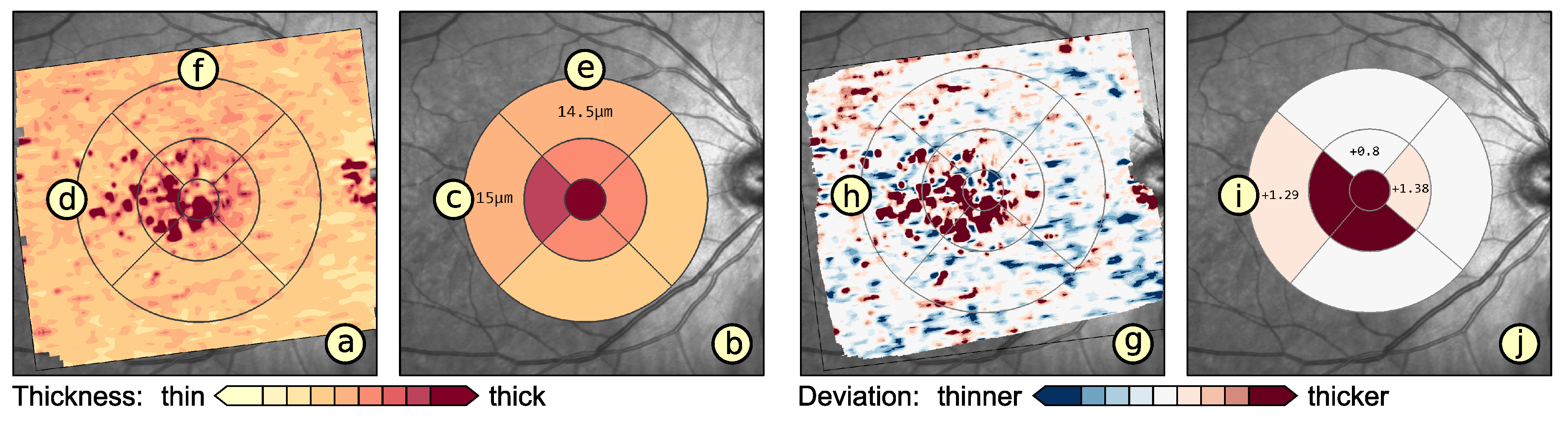
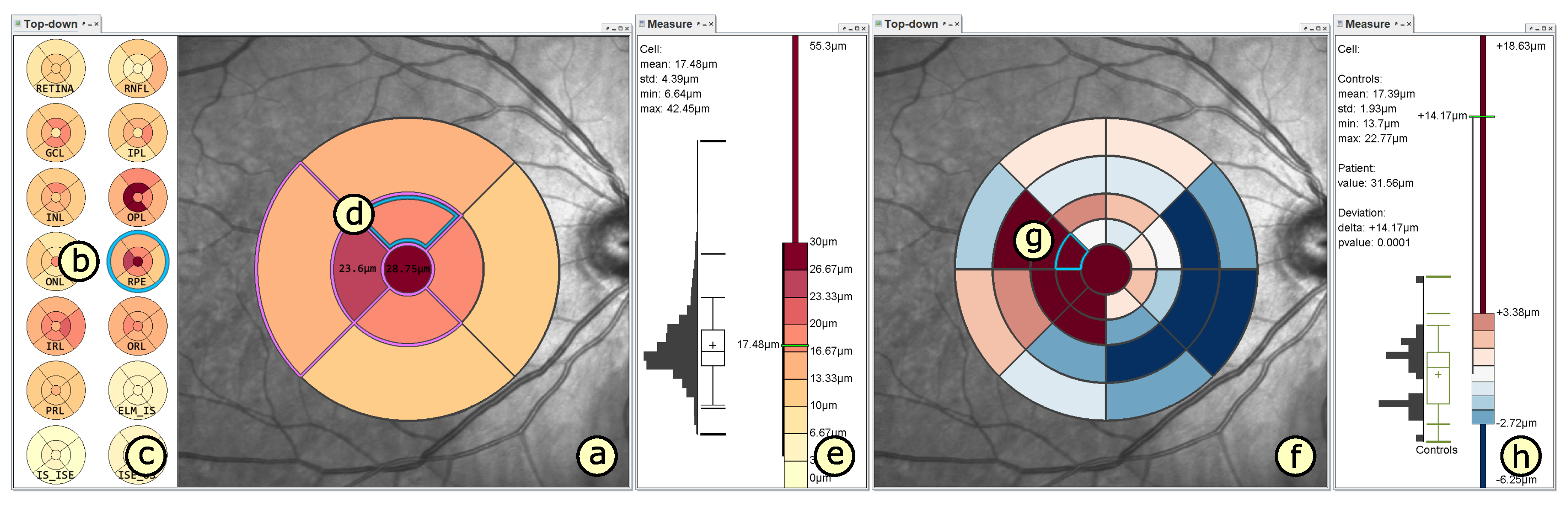
The visualization-related requirements correspond to the ophthalmologists’ goals when visually analyzing retinal thickness data. We devised suitable visualization concepts following a participatory design process. Together with ophthalmologists, we derived a list of design requirements and made general design decisions:

• Visualization in spatial context ($V{R}_1$): The thickness values of grids have to be presented in their underlying spatial frame of reference. This ensures that they are relatable to respective regions within the retina and allows to understand their spatial distribution.
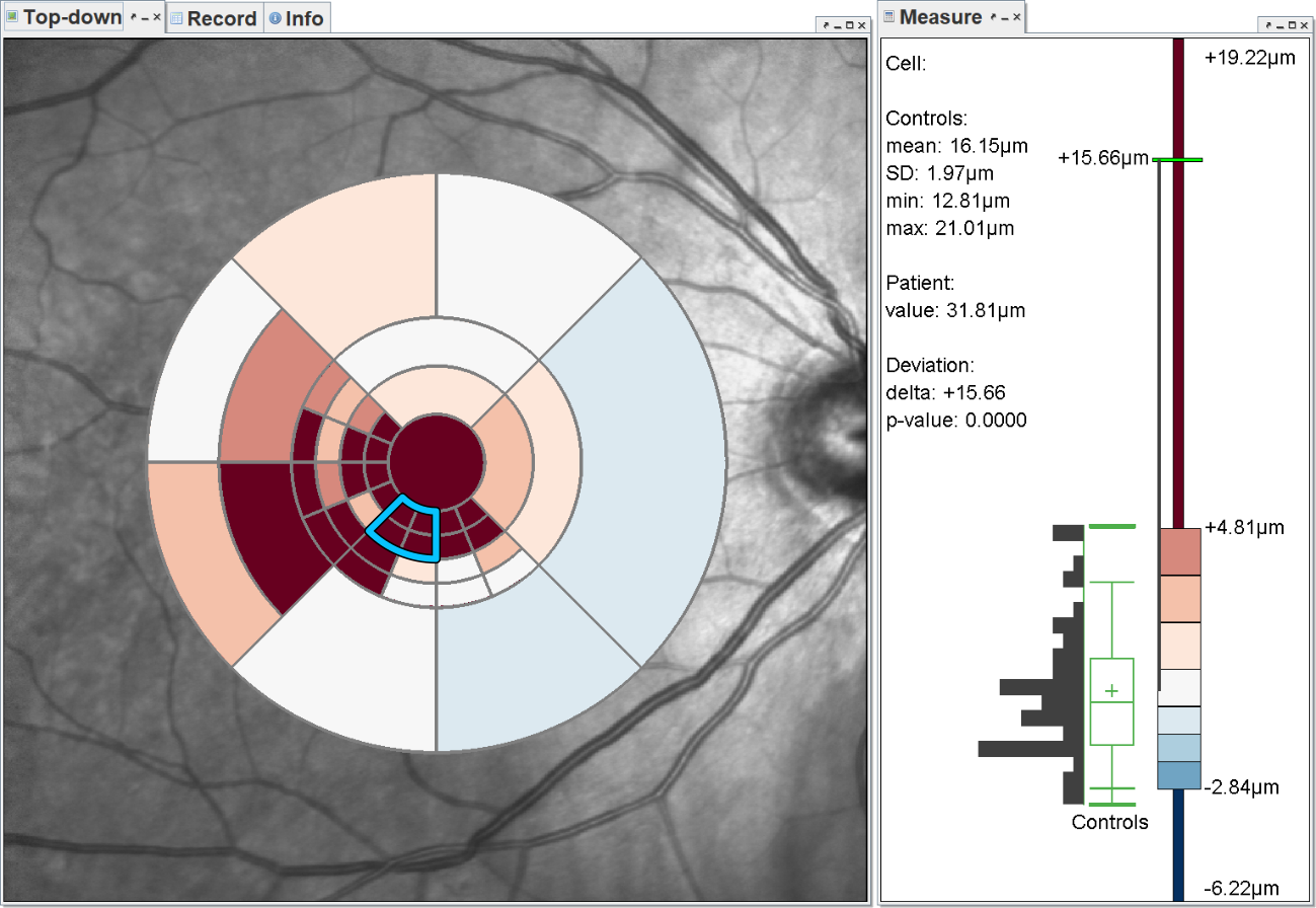
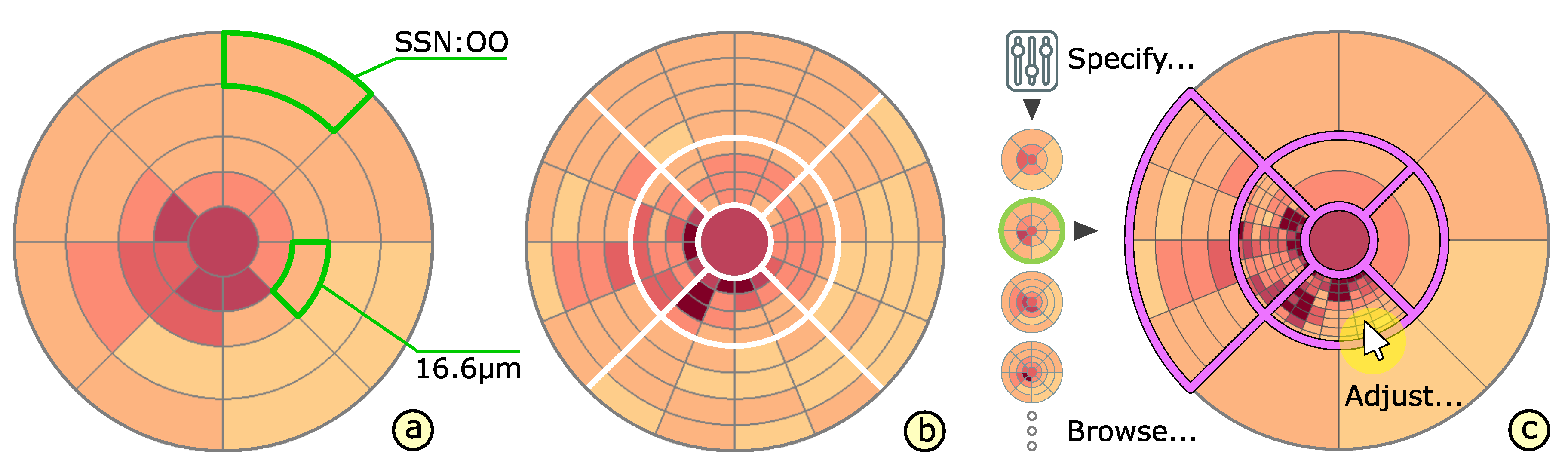
• Grid details on demand ($V{R}_2$): Details of grids with respect to space, e.g., finer subdivision of cells, and encoded information, e.g., the distribution of underlying thickness values, have to be made visually available upon request. This way, interactive investigations of findings at different levels of granularity are possible.
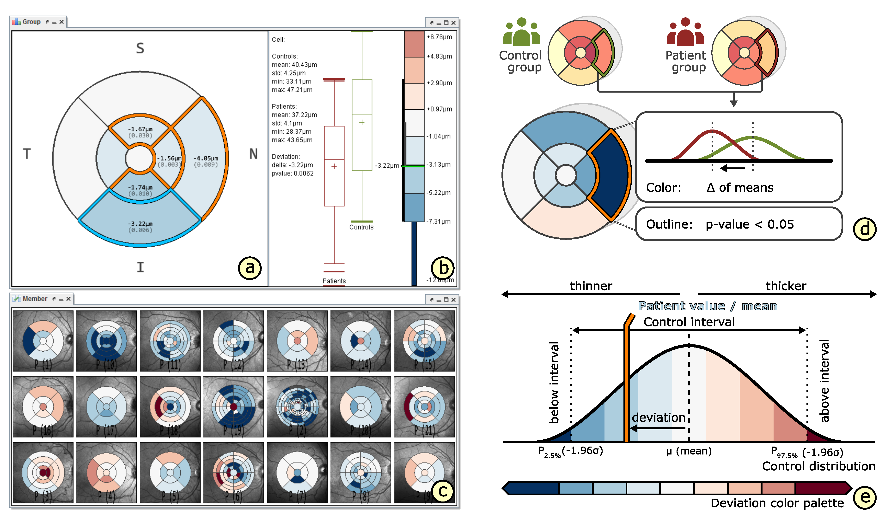
• Relation of multiple grids ($V{R}_3$): The thickness differences between multiple grids have to be graphically presented. In connection with the comparability of grid layouts (cf. $G{R}_2$), the differences need to be visualized in a common space. In case of ophthalmic studies, statistical quantification on top of a pure comparative display is required.

4.2. Presentation of Grids

The visualization design is based on multiple coordinated views. It includes a top-down view for coloring and labeling of grids and a measurement view for showing details of cells. With the linked first and second view, we address the visualization-related requirements $V{R}_1$ and $V{R}_2$.

The top-down view provides an overview of different thickness grids with regard to the interior surface of the eye (Figure 5a). A fundus image depicts the OCT acquisition area. On top, colored grids of selected retinal layers are visualized. The opacity of the grid overlay can be adjusted using a slider to relate cell values to noticeable structures in the fundus image. All other retinal layers are shown as grid thumbnails on the side, ordered according to their anatomical location within the retina (Figure 5c). This view design presents grids for all layers in one image without having to flip through them manually. Thus, layers with abnormal characteristics can be easily discovered.

The coloring of grids is based on suitable and adjustable palettes [32]. Sequential palettes encode the actual thickness of individual grids or the averaged thickness of aggregated grids. The cells are colored by evaluating the stored values with respect to clinically established thresholds. Two boundary values are given for all cells of each retinal layer. Low thickness values are assigned to light colors, high thickness values to dark colors, and thickness values outside the specified ranges to distinctively lighter or darker colors. Figure 5a shows an example. This allows to judge the thickness data globally in relation to the given boundaries. The coloring based on common thresholds also helps to relate grid presentations across different datasets.

The labeling of grids enriches the colored grids with additional text labels and highlighted cell borders. Text labels are added to show cell values in detail. Optionally, only text labels of selected cells or of cells with values outside of specified thresholds are displayed. This is to prevent visual clutter in the image, particularly in fine grids with a lot of small cells. Instead of showing numeric cell values, the labeling can be switched to encode location-oriented cell names (Figure 6a). To this end, existing naming conventions of the ETDRS grid (cf. Figure 1) can be adapted to derived grids. One alternative naming scheme is based on notations of points on a compass for directions and recursively partitioned macular rings for distances. For instance, a location is denoted by SSN:OO, which encodes a cell in the direction of superior superior-nasal (analogous to north northwest) at distance outer outer (outer half of outer macular ring) between the foveal center and the macular border. Next to text labels of cells, cell borders are outlined to illustrate the structure of grids and to highlight specific cells (Figure 6b). By default, all cell borders are outlined. The presentation can be adjusted to match selectively shown text labels of abnormal cells or to mark the ETDRS grid layout in subdivided grids. This further facilitates the localization of cells. Finally, cell borders may be emphasized to reflect the computed grid ratings, e.g., to indicate information loss in cells with low homogeneity (Figure 6c).

The measurement view goes beyond the basic grid presentation by showing further details of the thickness data (Figure 5e). Thickness values of selected cells in the top-down view are visualized as lines and numerical text labels on top of a color legend in the measurement view. The legend reflects the applied coloring and specified thresholds of the grid presentation. Next to the legend, summary statistics of selected cells are optionally shown as statistical plots. For individual grids, the distribution of the contained thickness data is visualized via box-and-whisker plots and histograms together with numerical labels of descriptive values. This helps to judge the grid representation and to understand the rating of cells, e.g., by showing the distribution of highlighted cells with low homogeneity. For aggregated grids, the statistical plots encode the distribution of thickness values of all corresponding source cells. This allows to assess the variability of thickness values of a group of patients.

4.3. Adaptation of Grids

To promote an in-depth data analysis, the thickness data have to be explored at an appropriate level of granularity. We support users in specifying initial grids to start the exploration, browsing through grids at different levels of granularity, and adjusting grids on demand. Figure 6c exemplifies the adaptation of grids. These interactive means address visualization-related requirement $V{R}_2$.

Specifying initial grids is possible in two ways: manually or automatically. The first option is based on interactive grid design, which gives ophthalmologists the greatest freedom and allows them to obtain grids that meet predefined needs. To manually specify a grid, the user has to set layout parameters, i.e., the number of radii and sectors. The second option is based on computed grid suggestions, which provide grids with the highest ratings of a number of alternative grid layouts. Alternative layouts may consist of increasingly finer subdivisions of the ETDRS grid using combinations of both radial and sector-wise partitioning strategies. Automated grid suggestions do not require user input. However, an ophthalmologist may steer the suggestions by setting additional constraints, e.g., the maximum number of allowed grid cells. This helps to obtain grids that adapt to variations in thickness but do not exceed a predefined level of granularity.

Browsing through grids is supported by interactive selections from a set of predefined grid layouts with different subdivisions. Selected grids are immediately shown in the top-down view with cells colored and labeled. By flipping through grids, the data are explored at different levels of granularity. For instance, selecting increasingly finer subdivisions of the ETDRS grid allows analyzing the data from an overview, i.e., the coarsest grid, to detail, i.e., the finest grid. This helps to understand the data and to localize areas of interest.

Interactively adjusting grids allows to refine or extend a predefined subset of grid layouts. On demand, one or multiple grid cells are selected and then merged together or subdivided by means of the provided partitioning strategies (cf. Section 3.2). This helps to fine-tune grids for given data based on the expertise of ophthalmologists. For example, while browsing through alternative grids, a specific grid is selected, cells are visualized, and information about the thickness data is shown. Individual grid cells with low ratings are further subdivided to investigate respective areas in greater detail and the remaining cells are merged together to provide context information of less relevant areas.

4.4. Comparison of Grids

Both a patient-specific and a group-specific analysis of retinal layer thickness requires the comparison of grids from multiple datasets. We enable such comparisons by juxtaposition of views, explicit encoding of deviations, and application of statistical tests. With the combination of these techniques, we address visualization-related requirement $V{R}_3$.

The juxtaposition of views supports the comparison of several individual grids (Figure 5a,f). In the user interface, multiple instances of the top-down view and measurement view can be dynamically added and freely arranged. For a patient-specific analysis, different grids of the same patient, e.g., follow-up examinations, or of related patients, e.g., similar medical cases, can be assigned to these view instances. Linking the view instances ensures that matching parts of the data are shown. For a group-specific analysis, grids of all individual members of a group are shown as small multiple views (Figure 7c). This provides an overview of differences between group members.

The explicit encoding of deviations facilitates a direct comparison of a grid to a reference grid (Figure 7d). For this purpose, the coloring of grids is switched. Diverging color palettes are used to encode cell value with respect to threshold intervals of an aggregated reference grid (Figure 7e). The boundary values vary cell by cell for each layer and are based on confidence intervals or percentile boundaries stored in reference cells. Small deviations are depicted via a light neutral color and larger negative or positive deviations via respective darker colors. Displaying deviations helps to evaluate a grid locally in relation to a reference grid. Figure 5f and Figure 7a exemplify comparisons of a grid of a single patient and of an aggregated grid of an entire patient group to intervals ranging between the 2.5^th and 97.5^th percentile boundaries of an aggregated grid of a control group, respectively.

The application of statistical tests allows to quantify differences between multiple aggregated grids. Different statistical tests are supported, e.g., Student’s t-test for quantifying differences between patients and controls or Tukey HSD test for multiple comparison between several patient subgroups and controls. The resulting measurements of statistical significance (p-values) and effect size are shown as numerical labels. Borders of cells with significant differences are highlighted with respect to a user-specified significance level, e.g., p < 0.05. In addition, statistical plots of cells for each grid under consideration are shown in the measurement view (Figure 7b). This illustrates respective thickness distributions and provides details of the color-coded deviations in the comparative grid presentation.

In summary, our grid exploration enables the analysis and comparison of the spatial distribution of retinal layer thickness at different levels of granularity. Our design helps ophthalmologists to perform in-depth data analyses and to interactively adapt them to their needs. On top of this, we develop a visual analysis tool that bundles our solutions in a flexible user interface and a complementary analysis procedure for evaluating ophthalmic study data.

5. Grid-Based Visual Analysis of Retinal Layer Thickness

We integrate our grid-based computation, visualization, and interaction techniques into a prototypical visual analysis tool for retinal OCT data. We demonstrate the utility of its main components in an analysis procedure for the evaluation of ophthalmic study data.

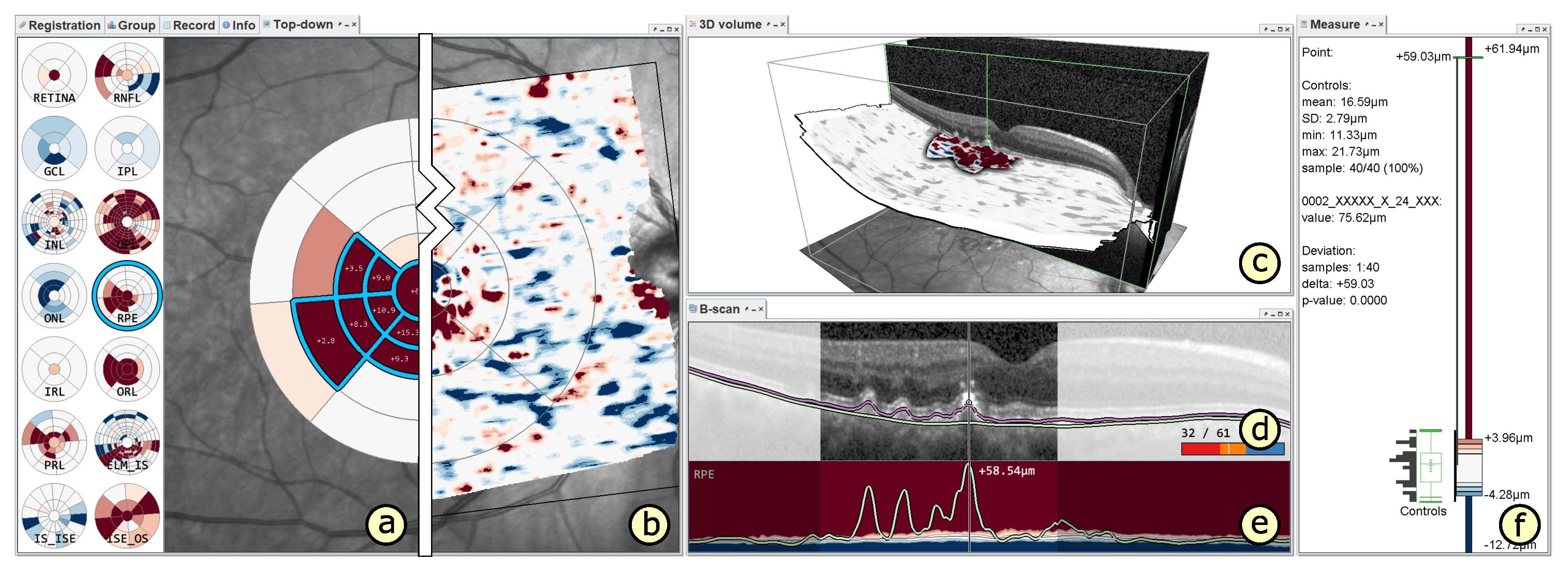
5.1. A Visual Analysis Tool

Offering our solutions in a visual analysis tool for retinal OCT data enables a comprehensive data analysis beyond the current use of thickness grids. The tool is a result of our previous work [26], which aimed at providing a unified interface for OCT data from different sources and an interactive visualization design for different aspects of OCT data, particularly with respect to thickness maps. We extend the available functionality and complement it with our grid design and exploration techniques. Figure 8 shows an overview of the user interface. The extended tool consists of three functional components for computation, visualization, and interaction:

The computation component combines diverse automated means for processing and analyzing retinal OCT data. Regarding our grid design, the computation of alternative grids, the rating of their representation quality, and the mapping and aggregation of grids are part of this component. It also provides a common data basis and parsing options for OCT data from different sources. Based on the converted data, layer thickness is derived together with other layer attributes, e.g., curvature, to characterize the condition of the retina. The thickness data are stored as maps or grids. Semiautomated registration methods allow to transform imported datasets into a common spatial frame of reference and to remove basic errors in the segmentation and thickness data. This enables precise comparisons of multiple grids or maps. Various statistical methods support the measurement, summarization, and quantification of grid cells or regions on maps.

The visualization component covers the necessary designs to present and visually relate different parts of OCT data, i.e., raw OCT data, segmentation data, and thickness data. Together with our grid exploration, three types of views are supported: a top-down view, a 3D view, and a cross-sectional view (Figure 8). The top-down view depicts thickness grids and maps with respect to their location within the retina. The 3D view displays OCT data and surfaces of segmented layers in a blended volume visualization. The cross-sectional view shows individual B-scans together with thickness profiles of selected layers. An extra measurement view provides additional information on cells, points, or regions selected in the other views. Supplementary methods for emphasizing spatial relationships and characteristic data values allow to show important information in the context of entire datasets. This includes information on the data quality, e.g., the signal strength of B-scans or invalid and missing values in the OCT data, segmentation data, and thickness data.

The interaction component supplies techniques that enable users to interact with the visualized data. This includes the adaptation and comparison of different grids. Comparisons of maps from individuals or groups are equally possible. Coordinated spatial and data-driven selections allow users to specify points, regions, cells, or value ranges of interest and to highlight them in the different views. Selections made in one view are automatically propagated to other linked views. For instance, selecting a grid cell allows to quickly access and relate respective locations on the surfaces of layers in the 3D view and associated B-scans in the cross-sectional view. To browse through the data, layers are switched or a cursor is moved in one view. The other views are updated accordingly and continuously display matched parts of the data. All navigation techniques are based on smooth animated transitions between camera movements to help users maintain their mental model of the visualized data.

The three functional components of our tool are implemented in a modular software architecture and a flexible user interface. The back end features a dedicated resource management that ensures efficient data processing and presentation. While most computations and renderings are performed on the fly (e.g., the adaptation of grids and automated measurements), some data preparations are preferably done offline (e.g., the initial registration and aggregation of many datasets). The front end supports stylizing the visualization and interactive exploration of retinal thickness data. This allows us to consider alternative display types, e.g., stereoscopic rendering to enhance the 3D perception of the spatial data. Altogether, our tool enables an interactive switch between different views, different levels of granularity, and two different tasks of analyzing individual patients and groups of patients.

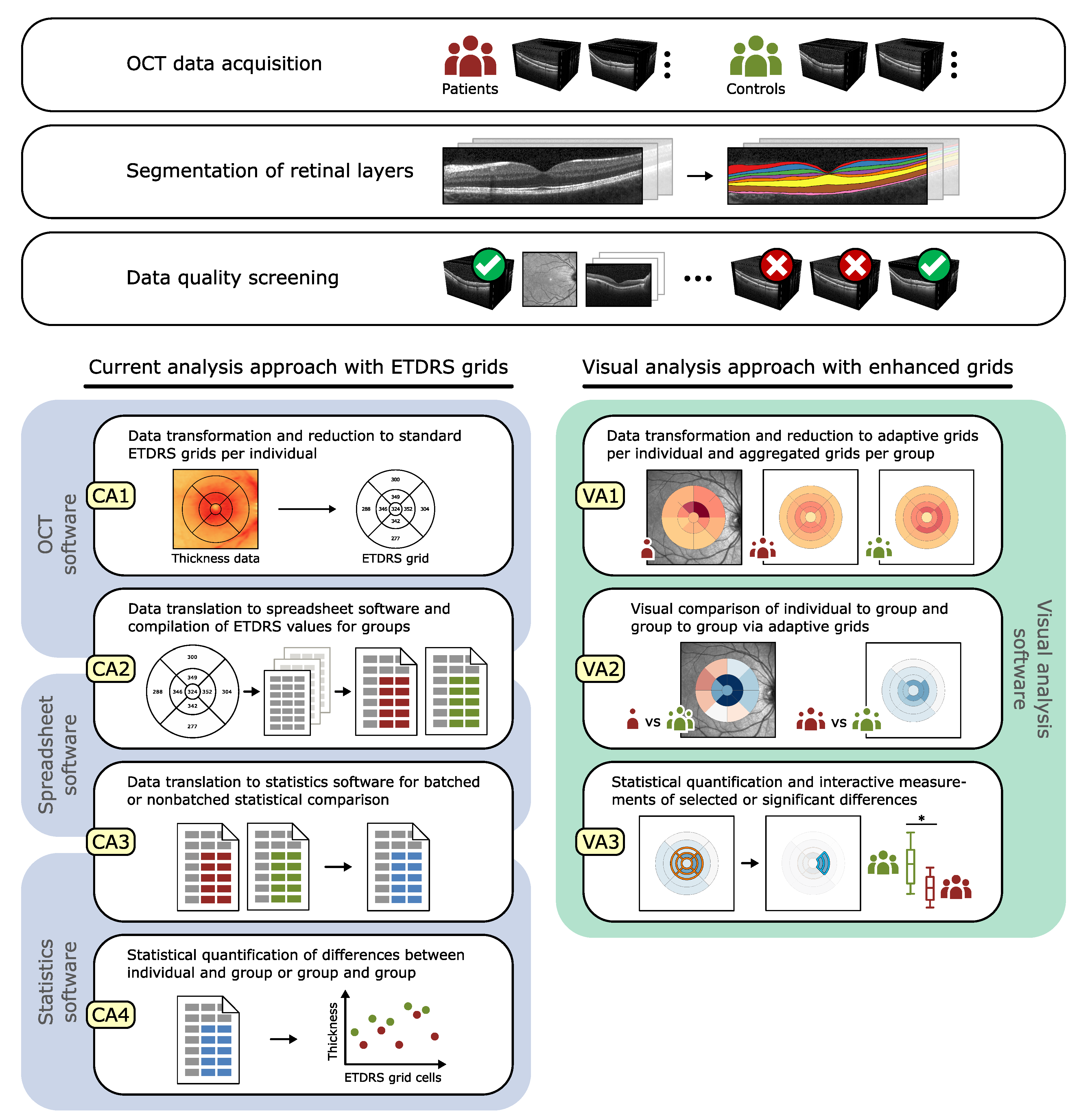
5.2. A Visual Analysis Procedure

To demonstrate our prototypical visualization tool, we developed an exemplary procedure for evaluating data from cross-sectional ophthalmic studies. In this connection, we discuss advantages and disadvantages of a current ETDRS-based analysis approach (CA) in relation to our enhanced grid-based visual analysis approach (VA). An overview of both methods is shown in Figure 9 and respective outcomes of two studies are described in Section 6.2. Together with ophthalmologists, we compiled the steps involved in CA and VA by observing and discussing data analysis practices. Four common analysis stages were identified: (1) data preparation, (2) data transformation, (3) comparison of patients and controls, and (4) quantification of findings.

In the first stage, the study data are prepared. Volumetric macular OCT images are acquired for every single subject and retinal layers are segmented using device-specific software. The image and segmentation data are screened to identify datasets with insufficient signal quality and erroneous or invalid layer boundaries. One or more best datasets per subject are selected and layer thickness data are computed for subsequent analyses.

In both CA and VA, data quality checks are crucial to prevent acquisition artifacts from impairing the data analysis. In CA, every dataset of every subject has to be validated one by one. This entails considerable manual effort, particularly in case of datasets with a high number of B-scans. A high density of B-scans is necessary for accurate retinal thickness measurements, prevention of interpolation errors [33], and capturing localized areas of retinal changes that occur in an early stage of a disease [34].

In VA, our tool provides additional support for displaying multiple datasets at once, indicating missing values and variations in signal strength, and highlighting and correcting segmentation errors [26]. Ensuring adequate segmentation quality is important in VA, as localized errors may become directly visible in smaller cells of subdivided grids. This is not necessarily the case in CA due to data aggregation in larger cells of ETDRS grids.

In the second stage, the study data are transformed. All datasets have to be registered and the thickness data are projected into a common spatial frame of reference. The registration is necessary to account for peculiarities of individual datasets, e.g., opposite laterality, tilted or off-center scan location, or different data resolution. Afterwards, the thickness data are reduced via given grid layouts.

In CA, data registration is performed by OCT device software. However, inter-individual positioning and laterality matching are often done by hand. Even though dedicated software options exist, their accessibility is limited because they are not supplied and installed as standard software features. The device software is then used for automated reduction of thickness data to standard ETDRS grids per layer and dataset (Figure 9, CA1). This provides a manageable amount of information per layer, which is easier to handle in the following data translation and statistical comparison of CA.

In VA, our tool offers semiautomated registration of datasets using the centers of the fovea and the optic disk as reference points [26]. Differences in laterality or resolution are compensated. Appropriate grid layouts are either generated based on the computed ratings or specified by the user. The thickness data are aggregated for each layer in datasets of individual patients, of entire patient and control groups, and of optional subgroups of patients (Figure 9, VA1). The adapted grids of individual patients provide a balanced representation of the thickness data. The aggregated grids of study groups are equally compact and precise and promote a cell-by-cell analysis with high spatial specificity. This aspect differs from CA in which data reduction and analysis based on ETDRS grids are applied.

In the third stage, the study data of patients and controls are compiled and compared. According to the study design, all data of investigated layers from individual subjects, subgroups, and groups are selected and assorted for the desired comparisons. After the comparisons, identified patterns are marked for further quantification and detail analysis.

In CA, this stage is divided into two steps. First, the study data are translated and exported from OCT software to spreadsheet software (Figure 9, CA2). The spreadsheet software is used for data fusion and compilation of groups or subgroups of patients and controls. Yet, the available export functionality can be limited. This is because, in our experience, OCT software from different manufacturers does not always provide an option to batch process multiple datasets and to export ETDRS grid values to external files, or such functionality is not activated by default. Hence, dozens of values per dataset may have to be copied by hand. This is time-consuming and error-prone, particularly in the context of larger studies with a lot of subjects. For example, in one case, more than 4000 data values were read from display of one software and manually copied to another software. Second, the compiled study data are again transferred to statistics software to perform batched or nonbatched statistical comparison (Figure 9, CA3). Typical comparisons are made either with respect to a fixed set of predefined study hypotheses or by computing and evaluating all potentially relevant combinations. The output of statistics software is summarized and reviewed in form of lists, tables, or statistical plots.

In VA, adapted grids of individual patients, subgroups of patients, and the patient and control groups are mapped and visually compared (Figure 9, VA2). The visualizations help to identify where exactly and to what degree retinal changes occur. This is a distinct advantage compared to CA, since changes in layer thickness of patients can be examined in their spatial context. First insights into the data are gained early in the overall analysis process and without the need for further data translation and export. The exploratory nature of VA does not necessarily rely on predefined study questions but rather assists in discovering patterns and investigating only involved layers and cells in detail. Typically, VA of study data starts by comparing the patient group to the control group to get a general idea of thickness deviation in patients. Additionally, other possible comparisons are between patient subgroups or between patient subgroups and the control group, which are helpful in identifying confounding factors that influence the study variables. Individual patients can also be compared to the control group, which is useful in understanding patient-specific retinal changes and tagging mild or severe cases. Optionally, our tool supports automated export of all or selected grid values of the study data to external files for further processing using external software.

In the last stage, findings are quantified and further investigated. Suitable statistical tests are applied to assess the observed differences in the comparisons of patients and controls. The most interesting findings are selected, graphically summarized, and reported.

In CA, statistics software provides various tests on top of the computed differences. Significant differences are highlighted in numerical lists or tables. Relevant results are then summarized via different types of charts, e.g., plots of mean deviation + standard error, that illustrate patient values in relation to controls for each ETDRS grid cell or ring (Figure 9, CA4). These tables and charts are useful to prove predefined study hypotheses and to draw study conclusions based on statistical numbers. The standardized ETDRS grid cells facilitate direct comparisons of statistical results from other studies. However, they do not disclose the presence or absence of localized variations in thickness, which were left unmeasured due to the applied data reduction in the earlier steps of CA. This may render the analysis results spatially unspecific.

In VA, statistical tests are applied to every grid cell and significant cells are highlighted in the compared grids. This way, the shape and extent of areas with significant differences can be accurately detected. The location and structure of significant cells in subdivided grids illustrate the spatial distribution of thickness changes. These unique patterns cannot be directly compared to statistical results of CA. Generally, it is only possible to compare the existence of smaller significant cells in relation to values of ETDRS grid cells. Although, based on our mapping of grids, VA results may be generalized and traced back to ETDRS results of CA if necessary. Our tool also supports interactive measurements of single or multiple cells to show statistical plots together with numerical labels of descriptive values. The measurements of cells in one grid are visually related to cells in another grid, e.g., cells of an individual patient to cells of a patient group. Further, the cells are shown together with the raw OCT data in the linked views of our tool. This interactive back and forth between comparisons, measurements, and adaptation of grids exemplifies the flexibility of VA. In contrast, if, after some analysis steps in CA, it turns out that a previous step has to be adjusted, the entire procedure must be reset to make the desired change and then repeated from that point on.

All in all, VA extends CA in several ways. Most importantly, it allows to reveal study-specific localized thickness differences between patients and controls. It also simplifies the overall analysis procedure by combining the computation and visualization functionality required for most analysis steps within a single tool. This is in contrast to CA, in which applied OCT software is mainly targeted at clinical practice, and thus ophthalmologists currently have to rely on a collection of diverse special and general purpose tools to evaluate study data. Moreover, the interactivity of our tool enables a flexible analysis process, which can be adapted on demand. Although, an extended support for data preprocessing in the first steps of the analysis procedure is required.

6. Application

We evaluated our research prototype in cooperation with ophthalmologists. Its utility was assessed in the context of one experimental and two cross-sectional studies. Following, we describe three use cases, present exemplary results, and reflect on benefits and limitations of our approach.

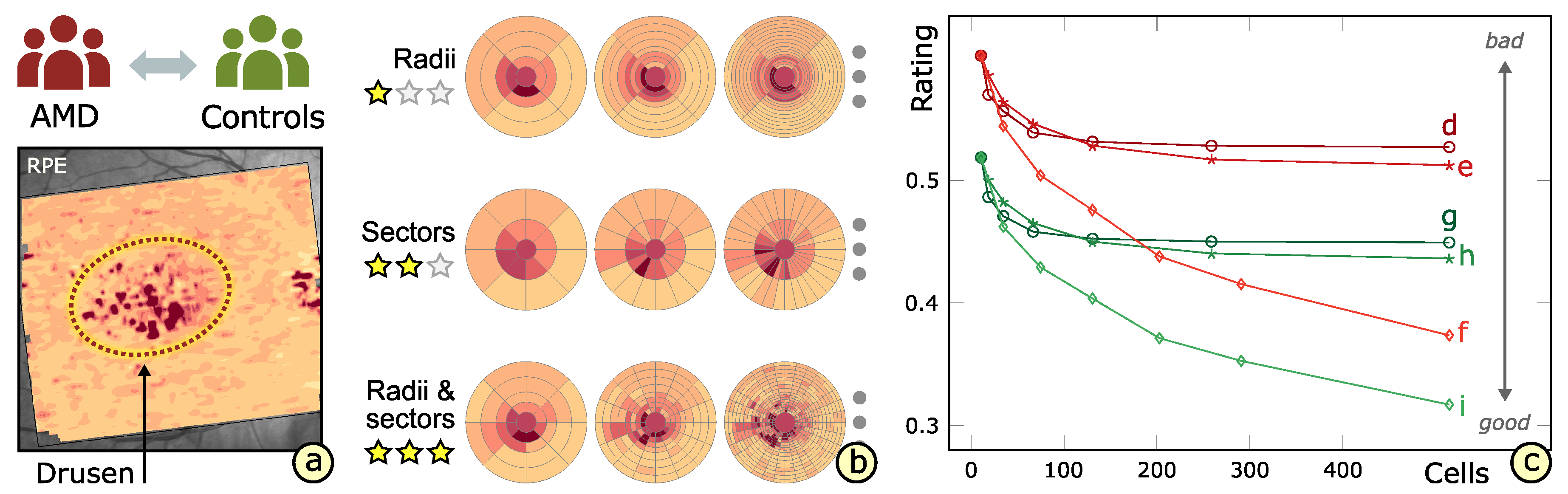
6.1. Experimental Evaluation of Patients with Age-Related Macular Degeneration

In this experimental use case, our principal goal was to demonstrate the feasibility of our approach. We applied our solutions to retinal thickness data of a small group of 8 adult patients suffering from age-related macular degeneration (AMD) and a group of 20 control subjects. We wanted to find out if early retinal changes related to AMD can be captured via different grid representations and how they relate to grid representation of healthy eyes. To reason about the utility of our approach, we assessed the obtained results from a data-centric perspective rather than conducting a comprehensive ophthalmic evaluation. Figure 10 illustrates the overall study setup and summarizes the findings.

An early sign of AMD is the presence of drusen in the macula. Drusen are small accumulations of extracellular material that build up between lower retinal layers of the eye [2] (Figure 10a). Particularly, in the thickness data of the retinal pigment epithelium (RPE), they become apparent as small and localized increases in thickness. We hypothesized that standard ETDRS grids are not always the best choice for representing the thickness data in such a setting (cf. Section 2.2).

To test this hypothesis, we specified 21 alternative grids and rated them with respect to thickness data of the RPE from patients and controls. For each partitioning strategy, 7 layouts with incrementally added radii, sectors, or radii plus sectors were included (Figure 10b). The numbers of radii and sectors were increased in constant steps up to a maximum of 129 radii, 256 sectors, and 17 radii plus 32 sectors, respectively. The finest grid layouts had 513 cells in each strategy. The ratings of the ETDRS grid and the alternative grids were first computed per subject and then summarized per layout to judge the overall representation quality for each group. In this connection, we assumed that a better rating is equivalent to a superior data representation based on the measures introduced in Section 3.4, i.e., a low mean standard deviation implies a good representation. Figure 10c shows the obtained results.

Generally, all alternative grids showed better ratings than the ETDRS grid. In patients, grids based on sector-wise partitions performed slightly better than grids based on radial partitions (Figure 10d,e). For both partitioning strategies, an increase in cell count only up to a certain point led to better ratings, suggesting that further added cells did not improve the representation quality of grids. In contrast, combined radial and sector-wise partitions showed continuously improved ratings with an increase in cell count (Figure 10f). We suspect that cells generated by this partitioning strategy more closely match the small, roughly circular-shaped regions of high thickness, which exist as a result of early drusen. In controls, the general trends in grid ratings per partitioning strategy were similar to those observed in patients (Figure 10g–i). This similarity can be explained by the consideration of patients with early AMD, i.e., patients with changes in layer thickness which are just noticeable but not significantly different from the control data. A remarkable difference, however, was that all control grids required fewer cells than the respective patient grids in order to obtain equally good ratings. We assume that this is due to the fact that thickness data of healthy eyes contain less localized variations in thickness and can be appropriately represented with fewer and coarser cells.

In summary, the alternative grid layouts provide a better representation of the studied thickness data of AMD patients. The results show that our approach allows us to determine suitable grids specifically tailored to each group. This indicates that a spatially-aware data subdivision helps to accurately characterize the condition of retinal layers.

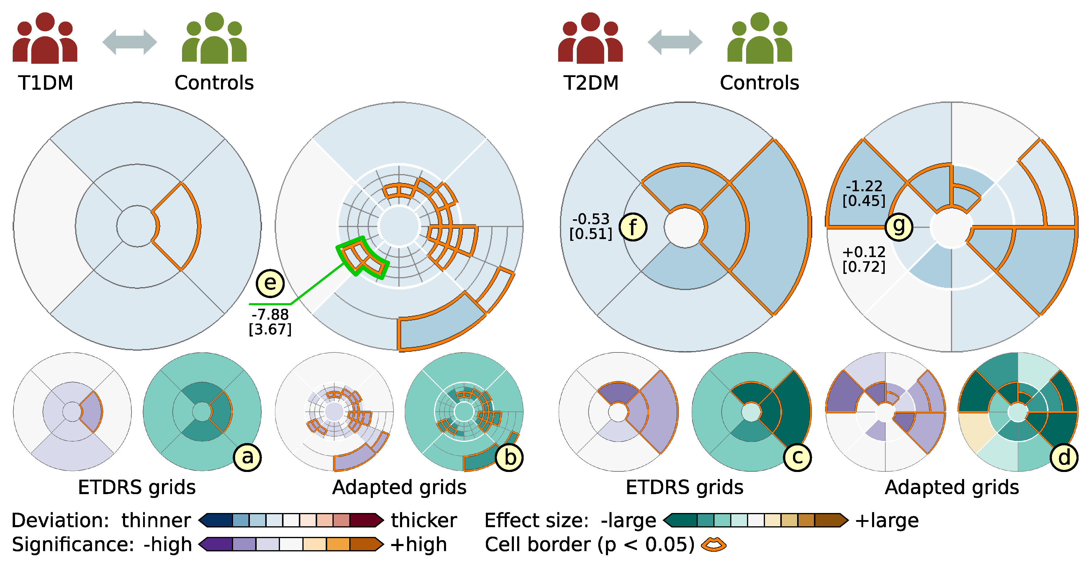
6.2. Grid-Based Analysis of Retinal Layer Thickness in Patients with Diabetes Mellitus

Motivated by the experimental results in AMD patients, we applied our solutions to analyze data of two other cross-sectional ophthalmic studies. The first study was focused on early retinal changes in pediatric patients suffering from type 1 diabetes mellitus (T1DM), and the second one on retinal changes in adult patients suffering from type 2 diabetes (T2DM). In both studies, the ophthalmologists were interested in evaluating the effectiveness of our enhanced grid-based exploration in comparison to a current practice of using only ETDRS grids for analyzing retinal layer thickness. In contrast to the experimental study, which focused on alternative grids to represent the actual thickness data per study group, the ophthalmologists specifically wanted to study how well abnormal thickness deviations of diabetic patients in relation to age-matched healthy controls are detected by each analysis method.

Previous ophthalmic studies have demonstrated deviations in the thickness of retinal layers in pediatric and adult patients with T1DM or T2DM [29,35]. These deviations in the thickness profiles of the retina serve as biomarkers or surrogate measures that aid an early detection and monitoring the progression of the disease. In an advanced stage of diabetes, the disease-induced alteration of layer thickness are expected to affect large retinal areas and exhibit a clear deviation from control data. In an early stage of diabetes, however, more subtle, localized, and scattered areas of thickness deviation are suspected that may go undetected without a spatially-aware subdivision and aggregation of the thickness data. Hence, we again hypothesized that such changes are not always adequately captured by a current analysis approach based on ETDRS grids. In fact, we were recently able to confirm the existence of localized areas of abnormal thickness in patients with early T1DM using a point-by-point data analysis based on deviation maps [27]. In the present studies, we aimed at obtaining similar results with our enhanced grid-based analysis, while reducing the data to a meaningful extent. The ophthalmologists also wanted to compare their findings in both studies to see if any general similarities between pediatric and adult patients with T1DM and T2DM exist.

The data of both studies were acquired via OCT examinations of each subject per group followed by retinal layer segmentation. In the first study, 26 pediatric T1DM patients and 29 age-matched controls participated and in the second study, 33 adult T2DM patients and 40 age-matched controls were involved. For each subject, the thickness data of total retina (TR) and inner retinal layers, i.e., retinal nerve fiber layer (RNFL), the ganglion cell layer (GCL), the inner plexiform layer (IPL), and the inner nuclear layer (INL), were selected for further investigation. For each selected layer, the ETDRS grid layout and one best fitting alternative grid layout were determined. One aggregated grid was computed per layout for every group in both studies. The resulting grids were then mapped and directly compared using explicit encoding of deviations together with statistical tests to quantify the differences between patients and controls (cf. Section 4.4). Lastly, based on the statistical results and computed grid ratings, the alternative grids were further adapted to investigate cells with significant differences in greater detail. Figure 11 shows exemplary results of the two studies.

Regarding the similarity of results in both studies, the ophthalmologists observed some common patterns. In general, they noted a significant amount of abnormal thinning in several investigated layers of both patient groups. In T1DM patients, cells with significant thinning were found primarily in the inner macular ring of TR and RNFL, and selectively in nasal direction of the outer macular ring. In T2DM patients, similar findings were made for TR and RNFL but also for GCL and IPL. The least amount of significant cells was detected for INL in both studies. These results are in accordance with results of other studies that reported thickness reduction of inner retinal layers in patients with T1DM (e.g., works by the authors of [29,36,37]) or T2DM (e.g., works by the authors of [35,38]) as an early event of neurodegenerative change.

Regarding the difference of findings between both studies, the ophthalmologists noticed a greater amount, spatial extent, and higher degree of significant thinning in adult T2DM patients than in pediatric T1DM patients. Particularly, they noted larger cells and darker cell colors (higher deviation) in subdivided grids of most layers in the T2DM study (e.g., grids of RNFL in Figure 11d). In contrast, subdivided grids from the T1DM group rather consisted of smaller cells due to a higher subdivision rate, hinting at the presence of more localized areas of abnormal thickness (e.g., grids of TR in Figure 11b). This is in line with our previous map-based findings of localized thickness changes in T1DM patients [27]. Possible reasons for the differences in the present study findings are the longer mean duration of disease in T2DM patients (T1DM: 5.6 years; T2DM: 13.3 years) and the inclusion of T2DM patients with mild to moderate diabetic neuropathy. A longer duration of diabetes together with an early diabetic neuropathy may have an effect on neuronal cells, which could explain the relatively greater amount and extent of thinning in retinal layers of T2DM patients. In this regard, further studies and analyses of correlations between thickness deviations and clinical parameters are necessary.

Regarding the comparison of analysis methods, our enhanced grid-based analysis and the standard ETDRS grid analysis both demonstrated general thickness changes of patients in relation to controls. However, the ophthalmologists pointed out a key difference between both methods: the enhanced grids revealed additional details of the distribution and degree of abnormal deviations, whereas the ETDRS grids failed to detect significant changes in certain areas. They also noticed a tendency of the ETDRS grids to underestimate changes (Figure 11f,g) and to produce false normal results in the studies. As an example, the neighboring fine cells of significant thinning crossing the inferior-temporal quadrants of the inner macular ring were only detected by the enhanced grid-based analysis (Figure 11b), but not as significant cells by the analysis based on the ETDRS grid (Figure 11a). In such a case, our design enables the measurement of multiple subdivided cells involving two or more quadrants within a macular ring (Figure 11e). Detecting and analyzing localized changes that span across boundaries of standard ETDRS grid cells was not possible with previous analysis methods. The measurement results allow to quantify the visualized data and help to get a greater understanding of a particular disease condition.

In summary, the enhanced grids are effective in detecting early and localized deviations in retinal layer thickness of pediatric and adult patients with T1DM and T2DM. The study results emphasize the importance of selecting an appropriate analysis method that supports a precise assessment of abnormal retinal alterations.

7. Discussion and Conclusions

We presented an enhanced grid-based reduction and exploration approach for retinal thickness data. Our solutions are a continuation of our previous work, in which we introduced the general design of our research prototype [26] and evaluated first studies using deviation maps [27,39]. Here, we extended this basis with a new grid design for precise detection of localized thickness variations and bundled the developed techniques in a flexible visual analysis tool. We also proposed a complementary analysis procedure to demonstrate the tool’s utility in the context of two cross-sectional studies. Collaborating ophthalmologists noted the added value of our solutions with respect to more findings and reduced manual analysis effort. We conclude that our approach offers a systematic enhancement of existing work and helps ophthalmologists in their grid-based analysis of retinal layer thickness.

So far, we implemented a data-driven approach to design grids and judge their representation quality. On the one hand, this offers high flexibility in balancing the granularity of grids and the amount of encoded information. On the other hand, automated grid suggestions are dependent on how well the employed quality measures, e.g., the standard deviation, quantify variations in the underlying thickness data. For some applications, very fine subdivided grids with a large number of cells may be practically unfeasible. On this account, our experimental evaluation method (cf. Section 6.1) helps to determine how much variance is acceptable in a grid with a certain amount of cells. This is particularly easy in case of grids that show no or only minimally improved ratings in further subdivisions with a certain partitioning strategy (e.g., Figure 10d,g). In contrast, suggesting best fitting grids in case of steadily improving ratings with an increase in cell count is more challenging and currently requires input by the user. This also applies to the grids generated via combined radial and sector-wise partitions in our experimental study of AMD patients, which showed better ratings compared to grids of other partitioning strategies (cf. Figure 10f,i). We will evaluate our grid-based methods in further studies to assess their reliability in relation to different patients and retinal conditions, and to share the collected medical insights in full detail with the ophthalmic community.

In this connection, an interesting extension is to establish a diagnosis-driven design and rating of grids. This requires custom strategies for measuring the quality of grids to target different ophthalmic analysis tasks. Moreover, default settings of layout parameters, e.g., the allowed maximum number of radii and sectors, and suitable rating cutoffs for the selection of best fitting grids have to be provided. Our ophthalmologists reported that they are trying to find new grid types that adequately represent retinal changes of specific diseases. A diagnosis-driven approach to rating and ranking of grids may support such efforts by evaluating newly designed grids and sorting out existing grid types.

We are also adapting the main ideas of our grid design and exploration to other basic grid types in specific ophthalmic applications. An example is the asymmetry analysis of retinal thickness data for glaucoma diagnosis using rectangular grids [31]. Currently, a standard 8 × 8 grid layout is used to analyze cell-by-cell differences in thickness between a superior and an inferior hemisphere. Figure 12 illustrates this application. Similar to the standard ETDRS grid, the predefined rectangular grid does not support an information-aware reduction of thickness data. Hence, we are extending and testing our grid design with respect to this grid type to support a fine-grained data analysis.

We further plan to augment our analysis procedure with other software tools. This will provide support for evaluating different types of ophthalmic studies. For example, in addition to retinal layer thickness, often other clinical parameters of patients are investigated. Typically, a diverse set of tools besides our solutions is required for preparation, analysis, and presentation of combined OCT data and clinical data. Fully integrating all tools into our software or replacing all their functionality with custom solutions is hardly possible. Instead, we follow a lightweight approach of loosely coupling individual tools into toolchains [40]. This way, ophthalmologists will be relieved from having to start, adjust, and transfer data to each required tool individually. In an initial effort, we are investigating the definition and execution of temporal tool sequences with an interactive editor.

References

1. Huang, D.; Swanson, E.A.; Lin, C.P.; Schuman, J.S.; Stinson, W.G.; Chang, W.; Hee, M.R.; Flotte, T.; Gregory, K.; Puliafito, C.A.; et al. Optical Coherence Tomography. Science 1991, 254, 1178–1181. [Google Scholar] [CrossRef] [PubMed] [Green Version]
2. Yoshimura, N.; Hangai, M. OCT Atlas; Springer: Berlin, Germany, 2014. [Google Scholar]
3. Keane, P.A.; Patel, P.J.; Liakopoulos, S.; Heussen, F.M.; Sadda, S.R.; Tufail, A. Evaluation of Age-related Macular Degeneration With Optical Coherence Tomography. Surv. Ophthalmol. 2012, 57, 389–414. [Google Scholar] [CrossRef] [PubMed]
4. Virgili, G.; Menchini, F.; Casazza, G.; Hogg, R.; Das, R.R.; Wang, X.; Michelessi, M. Optical coherence tomography (OCT) for detection of macular oedema in patients with diabetic retinopathy. Cochrane Database Syst. Rev. 2015, 1, CD008081. [Google Scholar] [CrossRef] [PubMed]
5. Grewal, D.S.; Tanna, A.P. Diagnosis of glaucoma and detection of glaucoma progression using spectral domain optical coherence tomography. Curr. Opin. Ophthalmol. 2013, 24, 150–161. [Google Scholar] [CrossRef] [PubMed]
6. Dörr, J.; Wernecke, K.D.; Bock, M.; Gaede, G.; Wuerfel, J.T.; Pfueller, C.F.; Bellmann-Strobl, J.; Freing, A.; Brandt, A.U.; Friedemann, P. Association of Retinal and Macular Damage with Brain Atrophy in Multiple Sclerosis. PLoS ONE 2011, 6, 1–6. [Google Scholar] [CrossRef]
7. Kashani, A.H.; Chen, C.L.; Gahm, J.K.; Zheng, F.; Richter, G.M.; Rosenfeld, P.J.; Shi, Y.; Wang, R.K. Optical coherence tomography angiography: A comprehensive review of current methods and clinical applications. Prog. Retin. Eye Res. 2017, 60, 66–100. [Google Scholar] [CrossRef] [PubMed]
8. Röhlig, M.; Stüwe, J.; Schmidt, C.; Prakasam, R.K.; Stachs, O.; Schumann, H. Grid-Based Exploration of OCT Thickness Data of Intraretinal Layers. In Proceedings of the 14th International Joint Conference on Computer Vision, Imaging and Computer Graphics Theory and Applications – Volume 3: IVAPP, Prague, Czech Republic, 25–27 February 2019; pp. 129–140. [Google Scholar] [CrossRef]
9. Costa, R.A.; Skaf, M.; Melo, L.A.; Calucci, D.; Cardillo, J.A.; Castro, J.C.; Huang, D.; Wojtkowski, M. Retinal assessment using optical coherence tomography. Prog. Retin. Eye Res. 2006, 25, 325–353. [Google Scholar] [CrossRef]
10. Hee, M.R.; Izatt, J.A.; Swanson, E.A.; Huang, D.; Schuman, J.S.; Lin, C.P.; Puliafito, C.A.; Fujimoto, J.G. Optical Coherence Tomography of the Human Retina. JAMA Ophthalmol. 1995, 113, 325–332. [Google Scholar] [CrossRef]
11. Drexler, W.; Morgner, U.; Ghanta, R.K.; Kärtner, F.X.; Schuman, J.S.; Fujimoto, J.G. Ultrahigh-resolution ophthalmic optical coherence tomography. Nat. Med. 2001, 7, 502–507. [Google Scholar] [CrossRef]
12. Choma, M.A.; Sarunic, M.V.; Yang, C.; Izatt, J.A. Sensitivity advantage of swept source and Fourier domain optical coherence tomography. Opt. Express 2003, 11, 2183–2189. [Google Scholar] [CrossRef] [Green Version]
13. Adhi, M.; Duker, J.S. Optical coherence tomography—Current and future applications. Curr. Opin. Ophthalmol. 2013, 24, 213–221. [Google Scholar] [CrossRef] [PubMed]
14. Cogliati, A.; Canavesi, C.; Hayes, A.; Tankam, P.; Duma, V.F.; Santhanam, A.; Thompson, K.P.; Rolland, J.P. MEMS-based handheld scanning probe with pre-shaped input signals for distortion-free images in Gabor-domain optical coherence microscopy. Opt. Express 2016, 24, 13365–13374. [Google Scholar] [CrossRef] [PubMed]
15. Drexler, W.; Morgner, U.; Kärtner, F.X.; Pitris, C.; Boppart, S.A.; Li, X.D.; Ippen, E.P.; Fujimoto, J.G. In vivo ultrahigh-resolution optical coherence tomography. Opt. Lett. 1999, 24, 1221–1223. [Google Scholar] [CrossRef] [PubMed] [Green Version]
16. Baghaie, A.; Yu, Z.; D’Souza, R.M. State-of-the-art in retinal optical coherence tomography image analysis. Quant. Imaging Med. Surg. 2015, 5, 603–617. [Google Scholar] [CrossRef] [PubMed]
17. Ehnes, A.; Wenner, Y.; Friedburg, C.; Preising, M.N.; Bowl, W.; Sekundo, W.; zu Bexten, E.M.; Stieger, K.; Lorenz, B. Optical Coherence Tomography (OCT) Device Independent Intraretinal Layer Segmentation. Transl. Vis. Sci. Techn. 2014, 3. [Google Scholar] [CrossRef] [PubMed]
18. Fujimoto, J.; Swanson, E. The Development, Commercialization, and Impact of Optical Coherence Tomography. Investig. Ophth. Vis. Sci. 2016, 57, OCT1–OCT13. [Google Scholar] [CrossRef] [PubMed] [Green Version]
19. Garvin, M.K.; Abramoff, M.D.; Wu, X.; Russell, S.R.; Burns, T.L.; Sonka, M. Automated 3-D Intraretinal Layer Segmentation of Macular Spectral-Domain Optical Coherence Tomography Images. IEEE Trans. Med. Imaging 2009, 28, 1436–1447. [Google Scholar] [CrossRef]
20. Mayer, M.A.; Hornegger, J.; Mardin, C.Y.; Tornow, R.P. Retinal Nerve Fiber Layer Segmentation on FD-OCT Scans of Normal Subjects and Glaucoma Patients. Biomed. Opt. Express 2010, 1, 1358–1383. [Google Scholar] [CrossRef] [Green Version]
21. Mazzaferri, J.; Beaton, L.; Hounye, G.; Sayah, D.N.; Costantino, S. Open-source algorithm for automatic choroid segmentation of OCT volume reconstructions. Sci. Rep. 2017, 7. [Google Scholar] [CrossRef]
22. Schindelin, J.; Rueden, C.T.; Hiner, M.C.; Eliceiri, K.W. The ImageJ ecosystem: An open platform for biomedical image analysis. Mol. Reprod. Dev. 2015, 82, 518–529. [Google Scholar] [CrossRef] [Green Version]
23. Garrido, M.G.; Beck, S.C.; Mühlfriedel, R.; Julien, S.; Schraermeyer, U.; Seeliger, M.W. Towards a Quantitative OCT Image Analysis. PLoS ONE 2014, 9, 1–10. [Google Scholar] [CrossRef] [PubMed]
24. Glittenberg, C.; Krebs, I.; Falkner-Radler, C.; Zeiler, F.; Haas, P.; Hagen, S.; Binder, S. Advantages of Using a Ray-traced, Three-Dimensional Rendering System for Spectral Domain Cirrus HD-OCT to Visualize Subtle Structures of the Vitreoretinal Interface. Ophthalmic Surg. Lasers Imaging 2009, 40, 127–134. [Google Scholar] [CrossRef] [PubMed]
25. De Fauw, J.; Ledsam, J.R.; Romera-Paredes, B.; Nikolov, S.; Tomasev, N.; Blackwell, S.; Askham, H.; Glorot, X.; O’Donoghue, B.; Visentin, D.; et al. Clinically applicable deep learning for diagnosis and referral in retinal disease. Nat. Med. 2018, 24, 1342–1350. [Google Scholar] [CrossRef] [PubMed]
26. Röhlig, M.; Schmidt, C.; Prakasam, R.K.; Schumann, H.; Stachs, O. Visual Analysis of Retinal Changes with Optical Coherence Tomography. Visual Comput. 2018, 34, 1209–1224. [Google Scholar] [CrossRef]
27. Prakasam, R.K.; Röhlig, M.; Fischer, D.C.; Götze, A.; Jünemann, A.; Schumann, H.; Stachs, O. Deviation maps for understanding thickness changes of inner retinal layers in children with type 1 diabetes mellitus. Curr. Eye Res. 2019. [Google Scholar] [CrossRef] [PubMed]
28. Early Treatment Diabetic Retinopathy Study Research Group. Grading Diabetic Retinopathy from Stereoscopic Color Fundus Photographs—An Extension of the Modified Airlie House Classification: ETDRS Report Number 10. Ophthalmology 1991, 98, 786–806. [Google Scholar] [CrossRef]
29. Götze, A.; von Keyserlingk, S.; Peschel, S.; Jacoby, U.; Schreiver, C.; Köhler, B.; Allgeier, S.; Winter, K.; Röhlig, M.; Jünemann, A.; et al. The corneal subbasal nerve plexus and thickness of the retinal layers in pediatric type 1 diabetes and matched controls. Sci. Rep. 2018, 8, 14. [Google Scholar] [CrossRef] [PubMed]
30. Chen, Q.; Huang, S.; Ma, Q.; Lin, H.; Pan, M.; Liu, X.; Lu, F.; Shen, M. Ultra-high resolution profiles of macular intra-retinal layer thicknesses and associations with visual field defects in primary open angle glaucoma. Sci. Rep. 2017, 7, 41100. [Google Scholar] [CrossRef] [PubMed]
31. Asrani, S.; Rosdahl, J.; Allingham, R. Novel software strategy for glaucoma diagnosis: Asymmetry analysis of retinal thickness. Arch. Ophthalmol. 2011, 129, 1205–1211. [Google Scholar] [CrossRef]
32. Harrower, M.; Brewer, C.A. ColorBrewer.org: An Online Tool for Selecting Colour Schemes for Maps. Cartogr. J. 2003, 40, 27–37. [Google Scholar] [CrossRef]
33. Odell, D.; Dubis, A.M.; Lever, J.F.; Stepien, K.E.; Carroll, J. Assessing errors inherent in OCT-derived macular thickness maps. J. Ophthalmol. 2011, 2011. [Google Scholar] [CrossRef] [PubMed]
34. Berufsverband der Augenärzte Deutschlands e.V.; Deutsche Ophthalmologische Gesellschaft; Retinologische Gesellschaft e.V. Quality assurance of optical coherence tomography for diagnostics of the fundus: Positional statement of the BVA, DOG and RG. Ophthalmologe 2017, 114, 617–624. [Google Scholar] [CrossRef]
35. Chhablani, J.; Sharma, A.; Goud, A.; Peguda, H.K.; Rao, H.L.; Begum, V.U.; Barteselli, G. Neurodegeneration in Type 2 Diabetes: Evidence From Spectral-Domain Optical Coherence Tomography. Investig. Ophth. Vis. Sci. 2015, 56, 6333–6338. [Google Scholar] [CrossRef] [PubMed] [Green Version]
36. Gundogan, F.C.; Akay, F.; Uzun, S.; Yolcu, U.; Çağıltay, E.; Toyran, S. Early Neurodegeneration of the Inner Retinal Layers in Type 1 Diabetes Mellitus. Ophthalmologica 2016, 235, 125–132. [Google Scholar] [CrossRef] [PubMed]
37. Tekin, K.; Inanc, M.; Kurnaz, E.; Bayramoglu, E.; Aydemir, E.; Koc, M.; Kiziltoprak, H.; Aycan, Z. Quantitative evaluation of early retinal changes in children with type 1 diabetes mellitus without retinopathy. Clin. Exp. Optom. 2018, 101, 680–685. [Google Scholar] [CrossRef] [PubMed]
38. Frydkjaer-Olsen, U.; Hansen, R.S.; Peto, T.; Grauslund, J. Structural neurodegeneration correlates with early diabetic retinopathy. Int. Ophthalmol. 2018, 38, 1621–1626. [Google Scholar] [CrossRef]
39. Stachs, O.; Prakasam, R.K.; Fischer, D.C.; Schumann, H.; Matuszewska, A.; Tschöpe, D.; Hettlich, H.J.; Röhlig, M. Visual Analytics of OCT data: Utility of deviation maps in describing retinal layer thickness changes. Investig. Ophth. Vis. Sci. 2019, 60, 1290. [Google Scholar]
40. Schulz, H.J.; Röhlig, M.; Nonnemann, L.; Aehnelt, M.; Diener, H.; Urban, B.; Schumann, H. Lightweight Coordination of Multiple Independent Visual Analytics Tools. In Proceedings of the 14th International Joint Conference on Computer Vision, Imaging and Computer Graphics Theory and Applications – Volume 3: IVAPP, Prague, Czech Republic, 25–27 February 2019; pp. 106–117. [Google Scholar] [CrossRef]
Figure 1. The layout of the standard ETDRS grid. The ETDRS grid cells divide the retina into nine regions defined by three rings and four quadrants (a). An overview shows the grid on top of a fundus image of a healthy left eye (b). The location of a B-scan is marked (central green line). A detail view shows the B-scan (c), segmented layer boundaries of total retina, and the layer thickness as a line chart (d). The dotted lines denote anatomically distinct areas along the image axis.
Information 10 00266 g001
Figure 2. Grid representation of retinal layer thickness. An OCT scan captures the area around the macula and the optic disk (a). Multiple B-scans are acquired (b). Retinal layers are segmented per B-scan (c) and thickness values are computed for every point along the horizontal image axes (d). The thickness values are combined per layer (e) and aggregated into thickness grids (f).
Information 10 00266 g002
Figure 3. Problems with an ETDRS grid-based data representation. The thickness of a retinal layer is shown via a thickness map (a) and an ETDRS grid (b). A cell (c) with localized regions of high thickness, visible in the map (dark red; d), has almost the same aggregated value in the grid as a cell (e) without such regions in the map (f). In the second map (g), localized regions of positive and negative deviations in thickness (dark red and dark blue; h) are nearly nullified due to data aggregation in corresponding cells (i) of the grid (j).
Information 10 00266 g003
Figure 4. Subdivision, mapping, aggregation, and rating of grids. The standard ETDRS grid layout is subdivided via radial (dashed line) or sector-wise (dotted line) partitions (a). A coarse grid is mapped to a fine grid or vice versa by subdividing or merging corresponding grid cells (b). Multiple source grids are compiled into a single aggregated grid (c). The representation quality of grids is rated by measuring the standard deviation of thickness values within each grid cell (d).
Information 10 00266 g004
Figure 5. Overview of our visualization design. In the left top-down view (a), a retinal layer (b) is selected in the layer overview (c) and an associated thickness grid is shown on top of a fundus image. Cell color encodes aggregated thickness values, labels indicate cell values close to specified thresholds, and borders of cells with low ratings are highlighted (purple). Details of a selected cell (d) are shown in a linked measurement view (e). In the right top-down view (f), a grid is mapped and compared to a control grid and deviations are color-coded. Details of a selected cell (g) are shown in a second measurement view (h) in relation to the control distribution.
Information 10 00266 g005
Figure 6. Interactive labeling and adaption of grids. The labeling of grids shows either numerical cell values or location-oriented cell names (a). White cell borders mark the layout of the standard ETDRS grid on top of a subdivided grid (b). The adaption of grids involves specifying initial grids, browsing through them, and adjusting cells of selected grids (purple borders) on demand (c).
Information 10 00266 g006
Figure 7. Comparison of grids. The top-down view (a) and linked measurement view (b) show a comparison between patients and controls via aggregated grids of both groups. The juxtaposed small multiple views (c) show an overview of grids of all individual patients in relation to controls. Patient values or group means are compared to the distribution of controls (d). A diverging color palette encodes differences per cell (e) and borders of cells with significant differences are highlighted (orange).
Information 10 00266 g007
Figure 8. A visual analysis tool for retinal layer thickness. A top-down view shows either grids (a) or maps (b). A 3D view presents a volume visualization of raw OCT data (c), and a 2D cross-sectional view displays individual B-scans (d) and thickness profiles of selected layers (e). All views are linked, selections in grids or maps are highlighted, and details are shown in a measurement view (f).
Information 10 00266 g008
Figure 9. Exemplary procedures for evaluating cross-sectional ophthalmic study data using an ETDRS-based analysis approach (CA) and an enhanced grid-based analysis approach (VA). After a common data preparation stage, CA comprises four analysis steps (CA1–CA4) with three software tools and VA involves three analysis steps (VA1–VA3) with our visual analysis tool.
Information 10 00266 g009
Figure 10. The experimental study setup and results in AMD patients and matched controls. Drusen are indicated by localized thickening in lower retinal layers of patient eyes (a). Examples of evaluated grids show increasingly finer subdivision of cells (b). The line plot (c) illustrates ratings of grids with respect to cell counts for thickness data of patients (red) and controls (green) in relation to three partitioning strategies: radial (d,g), sector-wise (e,h), and radial and sector-wise (f,i).
Information 10 00266 g010
Figure 11. Exemplary results of two cross-sectional studies. The grids represent TR in pediatric T1DM patients (a,b) and RNFL in a subgroup of adult T2DM patients (c,d) compared to matched controls. Cell color encodes thickness deviation, statistical significance, or effect size. Highlighted cell borders mark significant differences (p < 0.05). In T1DM patients, the ETDRS grids (a) depict significant thinning limited to a single cell. The subdivided grids (b) show additional cells of significant localized thinning and measurements of multiple small cells (e). In T2DM patients, the ETDRS grids (c) present a general overview of thickness deviation. The subdivided grids (d) show more details of the spatial distribution and degree of thinning. Some ETDRS grid cells underestimate the thinning (f) compared to corresponding subdivided grid cells (g).
Information 10 00266 g011
Figure 12. Asymmetry analysis of retinal layer thickness using rectangular grids. A standard 8 × 8 base grid layout (a) shows the mean difference between corresponding cells of opposite hemispheres (b). The fovea-to-disc axis (green line) marks the symmetry line and cell color encodes the degree of asymmetry (darker colors represent higher differences). In the upper grid half, negative differences between superior and inferior hemisphere are displayed and vice versa in the lower grid half. The subdivided grid (c) shows additional information on the spatial distribution and degree of differences.
Information 10 00266 g012