Article

A Two-Stage Household Electricity Demand Estimation Approach Based on Edge Deep Sparse Coding

School of Electrical and Electronic Engineering, North China Electric Power University, Changping District, Beijing 102206, China
*
Author to whom correspondence should be addressed.
Information 2019, 10(7), 224; https://doi.org/10.3390/info10070224
Submission received: 16 May 2019 / Revised: 10 June 2019 / Accepted: 24 June 2019 / Published: 1 July 2019

Abstract

:
The widespread popularity of smart meters enables the collection of an immense amount of fine-grained data, thereby realizing a two-way information flow between the grid and the customer, along with personalized interaction services, such as precise demand response. These services basically rely on the accurate estimation of electricity demand, and the key challenge lies in the high volatility and uncertainty of load profiles and the tremendous communication pressure on the data link or computing center. This study proposed a novel two-stage approach for estimating household electricity demand based on edge deep sparse coding. In the first sparse coding stage, the status of electrical devices was introduced into the deep non-negative k-means-singular value decomposition (K-SVD) sparse algorithm to estimate the behavior of customers. The patterns extracted in the first stage were used to train the long short-term memory (LSTM) network and forecast household electricity demand in the subsequent 30 min. The developed method was implemented on the Python platform and tested on AMPds dataset. The proposed method outperformed the multi-layer perception (MLP) by 51.26%, the autoregressive integrated moving average model (ARIMA) by 36.62%, and LSTM with shallow K-SVD by 16.4% in terms of mean absolute percent error (MAPE). In the field of mean absolute error and root mean squared error, the improvement was 53.95% and 36.73% compared with MLP, 28.47% and 23.36% compared with ARIMA, 11.38% and 18.16% compared with LSTM with shallow K-SVD. The results of the experiments demonstrated that the proposed method can provide considerable and stable improvement in household electricity demand estimation.

1. Introduction

Countries worldwide have committed to promoting and enhancing the efficiency and sustainability of power grids in recent years. Meanwhile, the widespread popularity of advanced metering infrastructure (AMI) enables the collection of an immense amount of fine-grained, real-time consumption data [1]. The effective management and analysis of AMI data can facilitate a bidirectional information flow and friendly interaction between customers and grids [2]. They also play a nontrivial role in accurate demand response (DR) [3], power reliability and efficiency improvement [4], electricity price design [5], and other personalized services [6,7].
The core of realizing these new services is to develop a highly accurate residential load forecast [8]. Two basic issues are associated with meter-level electricity consumption estimation. The first issue is the challenge of data transmission, numeration, and storage. Most power supply companies currently alleviate the tremendous pressure exerted on communication links and data storage computing power by simply reducing sampling frequency [9]. However, this method may result in the loss of effective information and cannot satisfy precision and rapid interaction requirements. Therefore, alleviating the communication and storage burden under the premise of ensuring the availability of effective information is a prerequisite for the effective analysis of energy consumption data [10]. The second issue is that high-resolution load data can no longer be limited to simple consumer segmentation (i.e., industrial, commercial, and residential) [11,12], but should further utilize hidden value or useful information to extract the electricity consumption behavior and lifestyle of consumers.
The data compression algorithm can be divided into lossless compression and lossy compression, depending on whether the original data can be restored after reconstruction. The reconstruction data are entirely the same as the raw data in lossless compression algorithms. By contrast, lossy compression is focused on similarity search and information extraction [13] and plays a nontrivial role in power load curve analysis [14]. Common lossy compression algorithms include discrete fourier transform (DFT) [15], discrete wavelet transform (DWT) [16], principal component analysis (PCA) [17], singular value decomposition (SVD) [18], and a combination of these methods. A load data compression method was proposed in [13], wherein the load status and other load characteristics were first introduced to process the data. The recoverable linear-time complexity data compression algorithm proposed in [19] is suitable for an error-prone transmission line. Focusing on smart meter data lossy compression, a non-negative k-means-singular value decomposition (K-SVD) algorithm was analyzed in [20], and the extracted behavioral patterns were used only to classify consumers into residents and small and medium-sized enterprises.
The electricity consumption behavior at the household or building levels has become a popular research topic in recent years. Compared with load profiles aggregated at high voltage levels, load profiles at the household level are frequently more volatile and sensitive to customer behavior or environmental variables, such as temperature, relative humidity, and their higher-order terms and interactions [21,22]. The load status of electrical appliances was first introduced to load forecasting in [23]. However, the sparsity of load data was not considered to pretreat the immense amount of original load data. Sparsity is a key characteristic in household-level load forecasting. Sparse coding was proposed to model usage patterns in [24]. The case study indicated that including sparse coding features led to a 10% improvement in forecast accuracy. A neural network prediction model with k-means clustering, which is a type of sparse coding algorithm, was used for load estimation in [25]. The K-SVD algorithm is a more flexible load curve coding method than k-means clustering. In this algorithm, the load curve can be represented as a superposition of several typical modes. In our previous study, an efficient edge sparse coding approach was proposed based on the K-SVD algorithm for extracting hidden behavior patterns from load datasets prior to load estimation to reduce communication, storage, and computation demands.
Deep learning has been applied in different industries, including smart grids. Designing deep learning structures for household load profile forecasting applications remains an open research issue in smart meter data analytics [26]. Theoretically, deep learning belongs to a type of special artificial neural network and focuses on extracting high-level features by applying appropriate nonlinear functions to hidden nodes to learn weights or filters in a greedy multi-layer [27]. However, features used for input data preprocessing in [26] were simply related to the sequence of energy consumptions and date, which may not reflect the user’s usage pattern effectively. In the current study, a two-stage household electricity demand estimation approach based on edge deep sparse coding was proposed by combining the concepts of deep learning and sparse coding. In the first stage, a 3-layer non-negative K-SVD algorithm with several representative household appliance load data was implemented to extract deep usage behavior patterns (DUBPs) as the input of the load forecasting. The load forecasting model based on long short-term memory (LSTM) was used in the second stage to realize accurate forecasting of household electricity demand. An edge sparse coding architecture to address the data deluge issue was also proposed, which most studies on load forecasting, including [26], did not consider. The deep K-SVD algorithm can be completed in the edge nodes and extracted DUBPs and the coefficient matrix can be uploaded to the cloud computing center for further load forecasting and storage.
From the preceding analysis, the contributions of this study were as follows.
(1)
A deep non-negative K-SVD algorithm, with an initial dictionary that consists of household electricity load, was proposed. This algorithm can extract deeper and more valid usage patterns that are conducive to the analysis and estimation of consumer behavior.
(2)
An edge sparse coding architecture was proposed to address the data deluge issue. In this architecture, deep sparse coding was completed in the edge nodes and then DUBPs or the coefficient matrix were uploaded to the cloud computing center for storage and estimation. This scheme considerably reduced the amount of data and effectively alleviated the communication and storage burden of the data link.
(3)
A novel two-stage estimation method for short-term household electricity consumption based on a LSTM network was proposed. Actual meter data were used for verification and simulation, and the results indicated that the proposed method achieved the best overall performance. It provided a considerable and stable improvement in load forecasting accuracy.
The remainder of this paper has been organized as follows. Section 2 briefly introduced the rationale for applying the deep K-SVD algorithm to usage pattern extraction and data pretreatment. Section 3 presented the two-stage household electricity demand estimation approach based on the deep K-SVD algorithm with household appliance data and LSTM. The edge sparse coding architecture was also designed for different calculation and storage capacities of edge nodes. Section 4 described the implementation of the experiment and case study using actual AMI data and compared the performance of the proposed approach with previous state-of-the-art methods, namely, autoregressive integrated moving average (ARIMA), multilayer perceptron (MLP), LSTM, LSTM with normal K-SVD, LSTM with 3-layer deep K-SVD algorithm and algorithm proposed in [23]. Finally, conclusions have been drawn in Section 5.

2. Deep K-SVD Algorithm

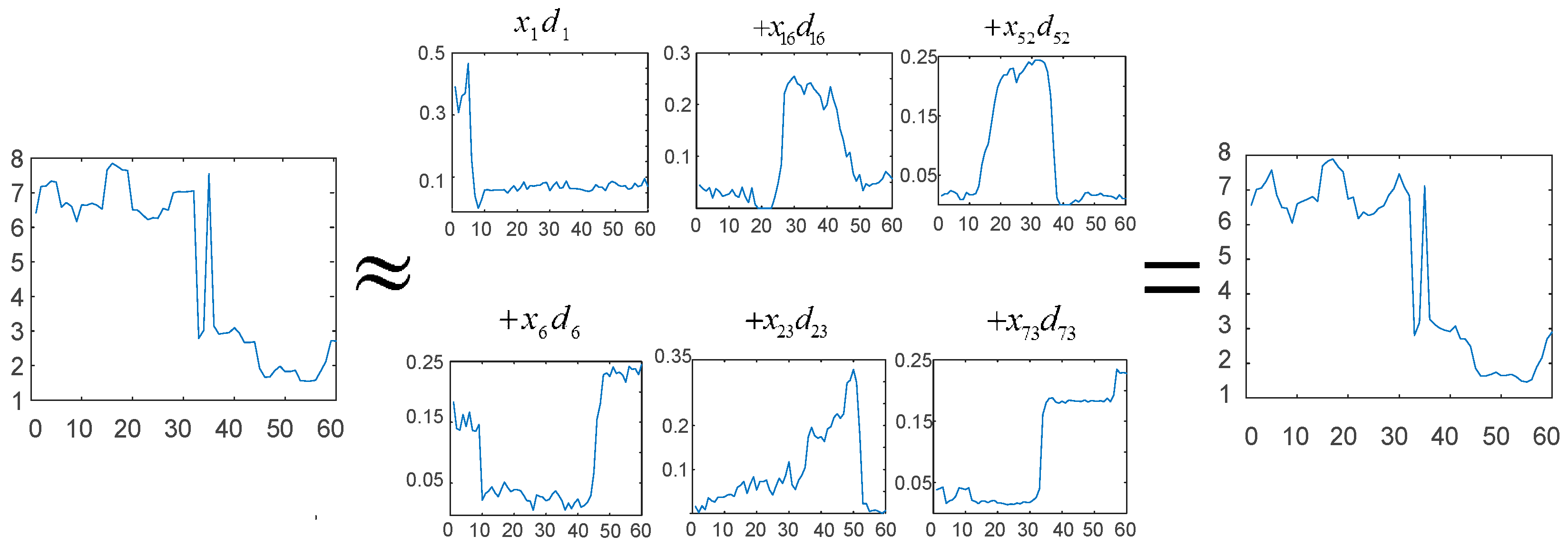
2.1. Basic K-SVD Algorithm

Data compression includes two phases—encoding and reconstruction. The encoder converts the original load curve to an optimal format with less storage space and restores the load curve with minimal reconstruction error. Sparse coding is inspired by the working mechanism of brain neurons [28] and attempts to obtain a sparse and redundant dictionary set to describe the characteristics of the original overall load.
Consider the given signal Y = [ y 1 , y 2 , , y M ] , which can be represented as a sparse linear combination of basic vectors in the overcomplete dictionary matrix D = [ d 1 , d 2 , , d J ] T . In the load analysis and decomposition problem, y i denotes the overall load and d j = [ d j , 1 , d j , 2 , , d j , N ] T is the jth UBPs, which has N dimensions same as the original signal. The sparse representation of Y can be described as
min D , X { Y D X F 2 } s u b j e c t   t o   i , x i 0 s 0 x i , j 0 , 1 i M , 1 j J d j , n 0 , 1 j J , 1 n N
where the basic vector d j = [ d j , 1 , d j , 2 , , d j , N ] T denotes the jth equipment behavior patterns, which has N dimensions same as the original signal. x i = [ x i , 1 , x i , 2 , , x i , J ] T is the coefficients vector of d j which only a few elements are nonzero to realize the dimensionality reduction of the original load signal [28]. The first constraints on s 0 is to ensure the compression efficiency of load profile and the second and third non-negative constraints on the coefficient vectors should be guaranteed because the UBPs are non-negative in practice.
The non-negative K-SVD algorithm is effective and flexible for solving the optimization problem in (1) or training the dictionary. The initial dictionary matrix should be predetermined, and the following steps should be repeated until the required number of iterations is reached or the constraints are satisfied.
(1)
Sparse coding: The orthogonal matching pursuit (OMP) algorithms are introduced to obtain the approximate solution of the sparse coefficient vector x i that corresponds to each load profile y i .
x ^ = a r g   m i n y D x ^ 2
(2)
Dictionary updating: The dictionary vector is updated with fixed coefficient vectors.
Figure 1 shows a visualization of sparse coding, where the original signal is finally represented by a linear combination of six UBPs. Notably, the number of columns in the feature dictionary, J, should be greater than the number of rows in the original signal N, which is determined by the redundancy of the dictionary. The sparsity of sparse coding is primarily reflected by the condition that most coefficient vectors are zero.

2.2. Deep K-SVD Algorithm

The basic K-SVD algorithm has a shallow architecture and only learns one dictionary level. In this section, the authors proposed to extend shallow dictionary learning into multiple layers, thereby leading to deep sparse coding. Deep dictionary learning is performed by using a greedy approach to continuously find the sparse representation of the coefficient matrix until the last layer is reached. This deep non-negative K-SVD algorithm can extract deeper and more valid DUBPs and is more conducive to analyzing and estimating costumer behavior. The schematic of deep DUBPs extraction is shown in Figure 2.
In the greedy solution, the coefficient matrix learned in the i th layer X i can be substituted as X i = D i 1 X i 1 until i = L 1 (for L layers), whereas the sparse representation problem in the (i + 1)th layer can be expressed as:
min D i 1 , X i 1 { X i D i 1 X i 1 F 2 }
Hence, the multi-level dictionary learning problem with non-linear activation can be formulated as:
min D , X { Y D 1 D 2 D L X L F 2 } s u b j e c t   t o   i , x i 0 s 0 x i , j 0 , 1 i M , 1 j J d j , n 0 , 1 j J , 1 n N
where D = D 1 D 2 D L is the DUBPs extracted by deep K-SVD algorithm [29].
In summary, the deep sparse coding algorithm provides two major improvements in calculating electricity consumption. First, it can obtain a multi-layer overcomplete dictionary, called DUBPs library in this study. DUBPs can be maximally consistent with users’ actual electricity consumption behavior through continuous training. Second, the coefficient vector can be optimized L times to reduce reconstruction error while obtaining an over-complete sparse dictionary. Therefore, the corresponding DUBPs are also more consistent with the actual consumption of users.

3. Proposed Methodology

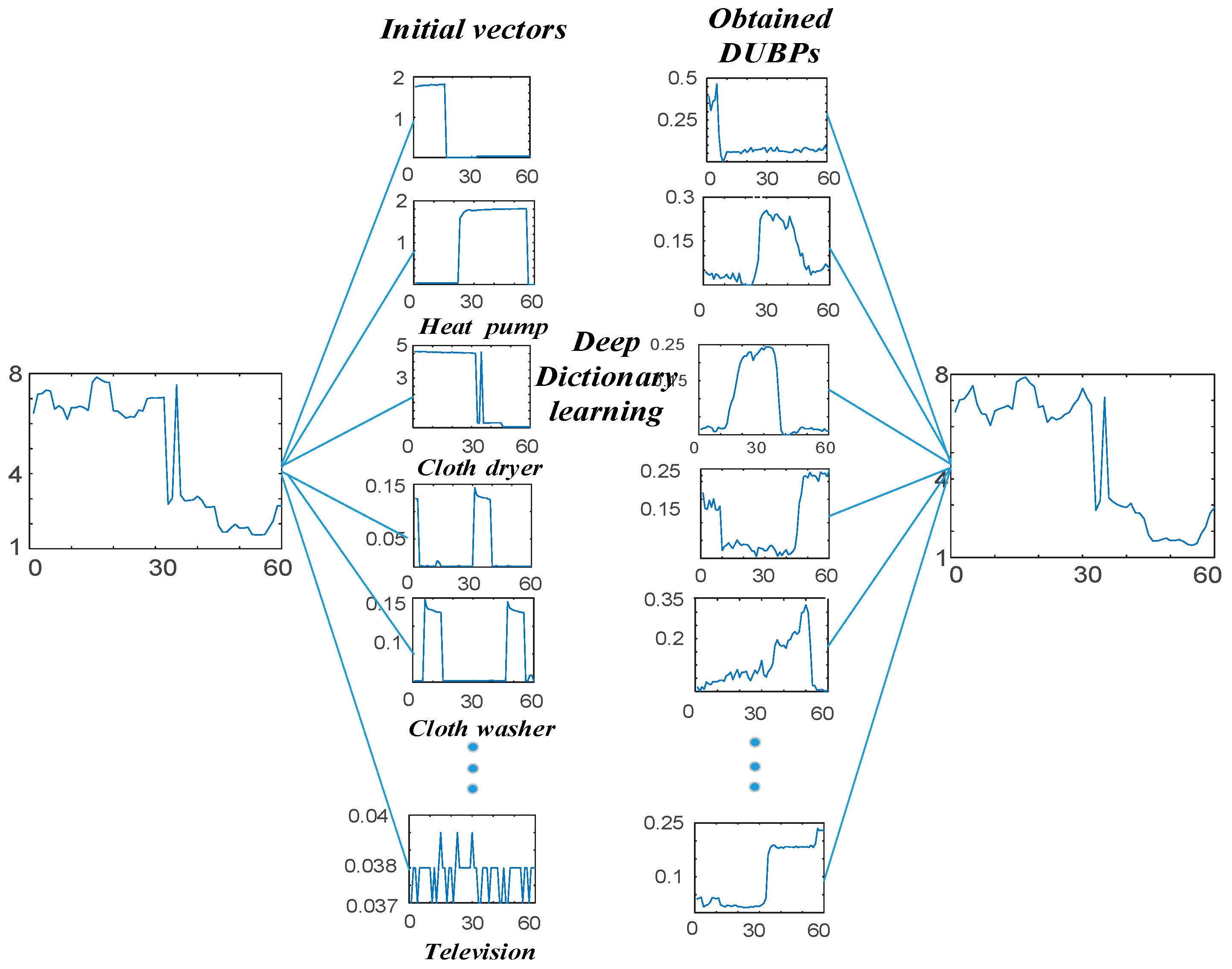
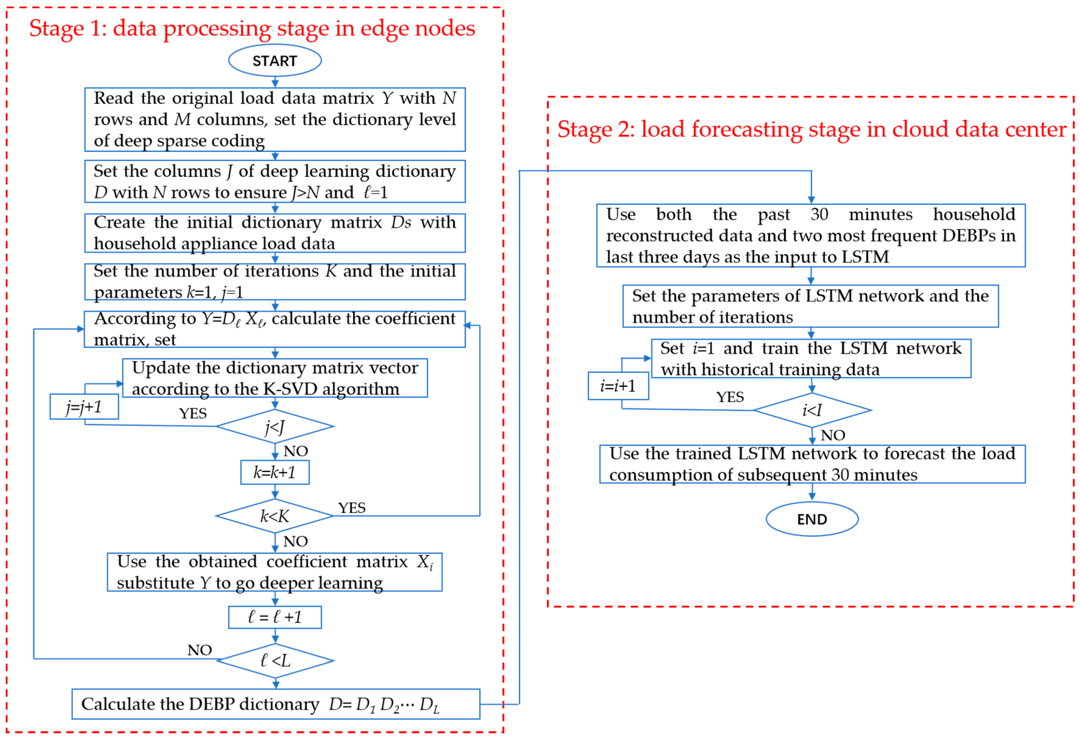
3.1. Stage 1: Deep K-SVD Algorithm with Household Appliance Data

In the first stage, the deep non-negative K-SVD algorithm was implemented for load profile compression and DUBPs extraction. DUBPs were fed into the second stage as input to enhance the efficiency and stability of load forecasting.
The construction of a suitable initialization dictionary D s is a kernel point in the sparse coding problem. Current studies have generally used a part of the original signal or classical bases (e.g., Fourier and Gaussian bases) as the initial dictionary matrix. The signature of electrical devices was first introduced to load forecasting in [23], and the experiment showed that a combination of historical load and household appliance data can considerably enhance the forecasting of individual consumer loads. The sparse coding process with appliance load is illustrated in Figure 3. This study selected the load profiles of several representative appliances related to the lifestyle of residents as the initial dictionary matrix to satisfy the diversity of actual loads.
Houses equipped with sub-meters can obtain noiseless household appliance consumption profiles. Load disaggregation or non-intrusive load monitoring (NILM) technology is applied to recognize the consumption of each appliance when only the overall current or load reading is available [30]. Unlike the submetering, appliance consumption gathered by NILM is noisy. This study hypothesized that when the load of appliances has been gathered, the initialization dictionary matrix can be defined as:
D s = ( a 11 a 1 n a m 1 a m n b 11 b 1 n b m 1 b m n c 11 c 1 n c m 1 c m n d 11 d 1 n d m 1 d m n )
where a 11 a m n , b 11 b m n , c 11 c m n , and   d 11 d m n denote the load of four electrical appliances. The values of m and n are determined by the dimension of the original signal and the size of the dictionary matrix, respectively.
The load of the electrical devices is added to the deep non-negative K-SVD sparse coding to obtain an over-completed dictionary, where DUBPs must be consistent with actual customer behavior as much as possible, and the coefficients must be optimized to simultaneously ensure sparsity and reduce the reconstruction error.

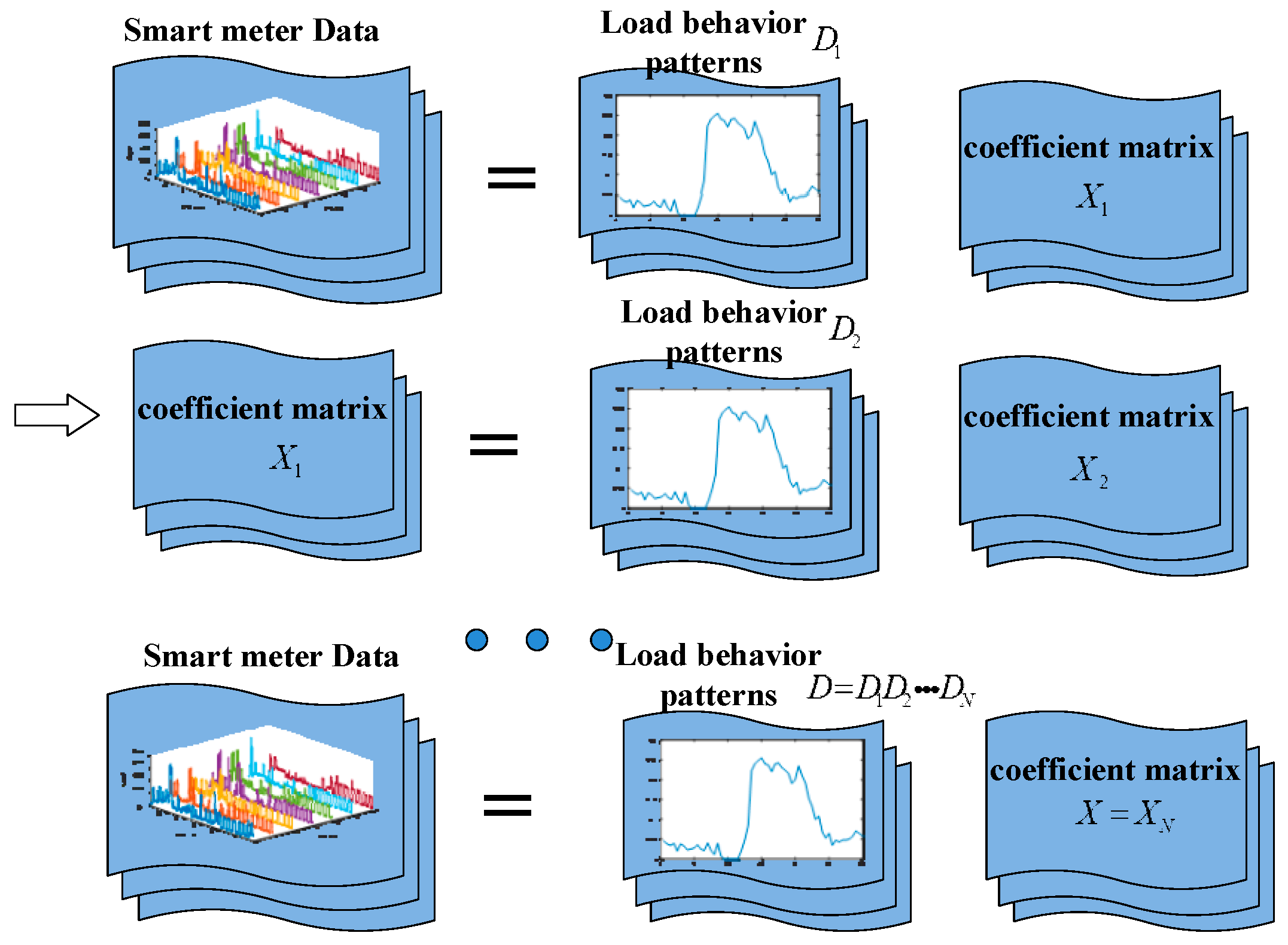
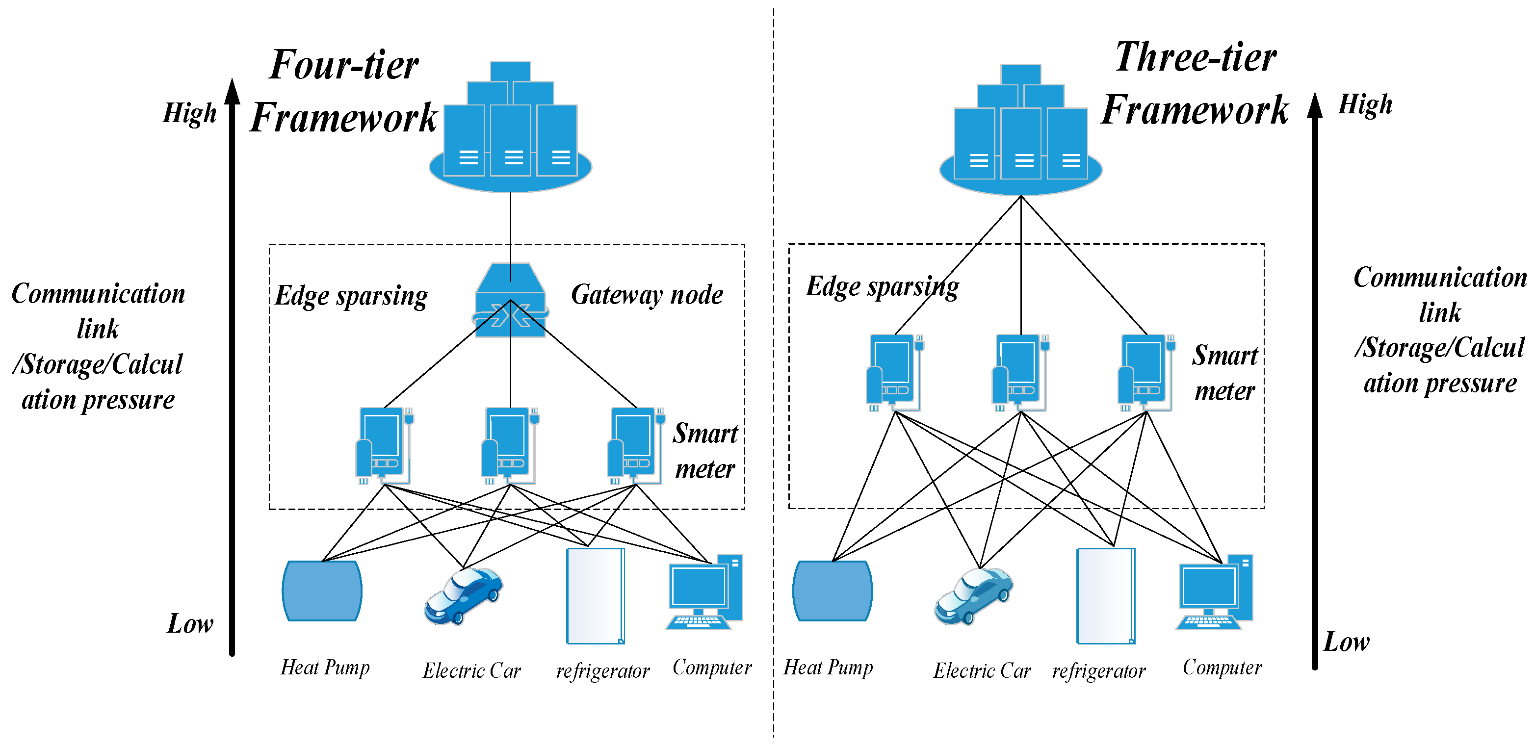
3.2. Edge Sparse Coding Architecture

Edge computing is a concept of near computing, that is, the operation is completed in the local network which is closer to the data source [31]. However, not all data operations can be placed on the local side, and some data still require further analysis or long-term access to transfer back to the cloud computing center for processing or storage. The cloud computing center can be similar to a central coordinator or a data training center in the future.
Evidently, the pressure exerted by communication, calculation, and storage gradually increases along the data link from local meters to the cloud computing center. Smart meters and gateways exhibit certain analysis and calculation abilities and can perform the data compression task. In such cases, the transmission pressure on the data link and cloud computing center can be substantially alleviated. Therefore, a sparse coding architecture based on edge computing was introduced, as shown in Figure 4, where the deep K-SVD algorithm was completed in the edge nodes. Deep sparse coding requires higher computing and storage capacities than single-layer sparse coding. The edge sparse coding architecture can be three-tier or four-tier, depending on the capacity of the smart meters. The edge nodes of the three-tier sparse coding structure are smart meters only, whereas smart meters and a gateway play the role in the four-tier computing architecture to improve the data-handling ability of edge nodes. The extracted DUBPs and coefficient matrix are uploaded to the cloud computing center for load forecasting and storage.
The advantage of the proposed edge sparse coding architecture is manifested in the following aspects: (1) The amount of data is considerably reduced after edge sparse coding, which will substantially contribute to alleviating communication and storage burden; (2) the major modifications occur at the grid side and exert minimal impact on customers; (3) this scheme can be implemented by directly installing a sparse coding module on existing smart meters or adding an intelligent gateway with data computing capability. It does not substantially change the existing electricity distribution network and considerably reduces procurement and construction costs.

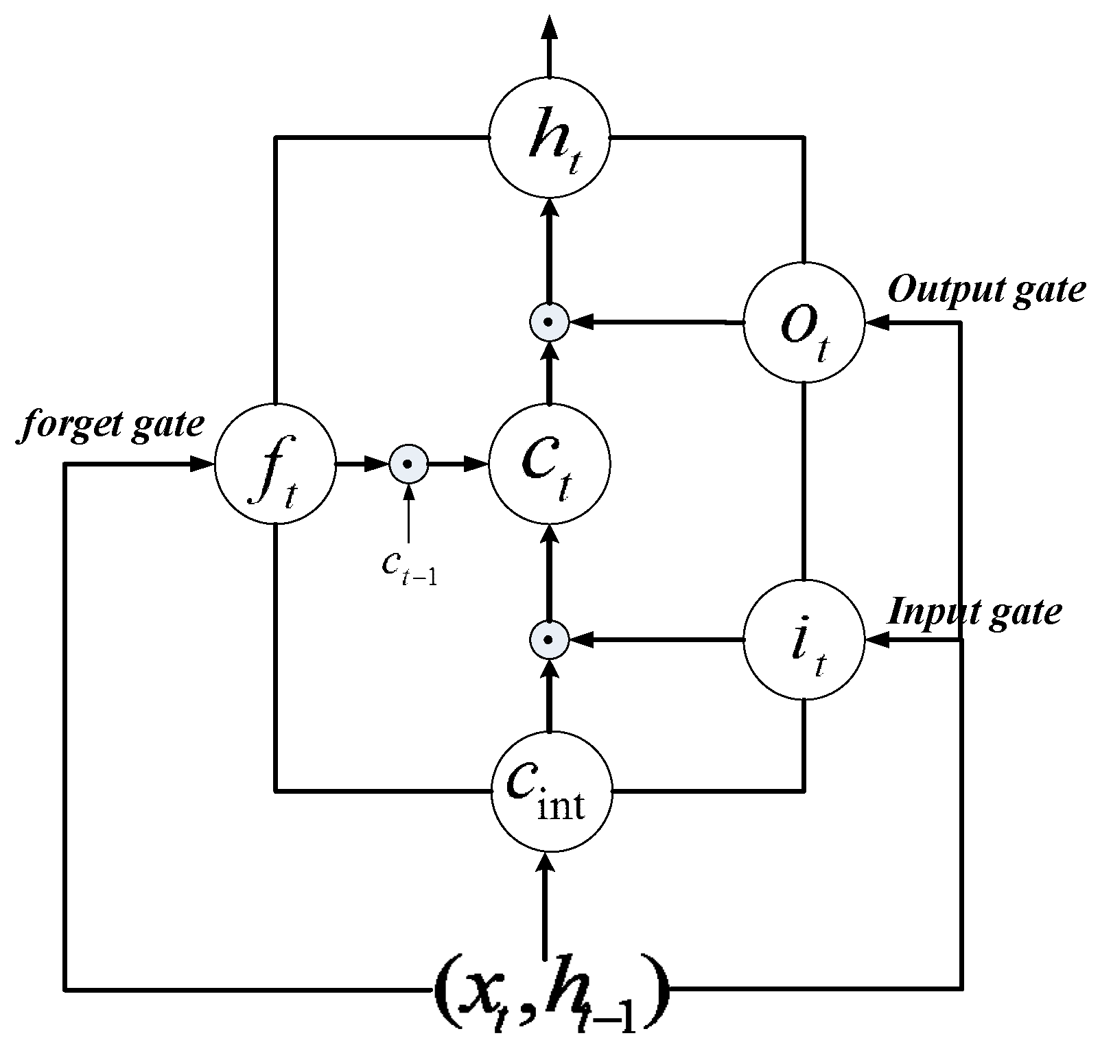
3.3. Stage 2: DUBPs-Based Electricity Demand Estimation Using LSTM

This stage of the proposed method consisted of training and testing DUBP-based load forecasting. In the training part, the reconstructed household data for the past 30 min and two DUBPs extracted from the load profile using the edge deep sparse coding algorithm were used to train the LSTM network. In the testing part, the well-trained LSTM network was implemented to forecast household electricity demand in the subsequent 30 min. Household-level load demand estimation is critical for precise DR. However, accurate forecasting is difficult due to the variability and randomness of resident behavior. LSTM was selected because it can be flexible for the strong temporal correlation of household-level load data.
An LSTM network refers to a specific architecture of recurrent neural network (RNN). It not only exhibits the recursive attribute of RNN, but also includes a unique memory cell with an additional forget gate, which solves the gradient vanishing or exploding problem in traditional RNN. LSTM networks have achieved considerable success and are currently popular in many sequential forecasting tasks.
Both LSTM network and traditional RNN are composed of an input layer, an output layer, and a hidden layer. However, the hidden layer of an LSTM network is no longer a common neural unit, but a recurrent memory unit. Figure 5 presents a typical LSTM cell.
Let x = { x 1 , x 2 , x T   } denote a typical input sequence for an LSTM network, where x t k represents a k -dimensional vector for actual values at each time step t . To establish temporal connections, LSTM defines and maintains an internal memory cell unit at each time step t as a collection of vectors in k : an input gate i t , a forget gate f t , an output gate o t , a memory cell c t , and a hidden state h t .
The memory cell state c i n t interacts with the intermediate output h t 1 , and the subsequent input x t in the input gate, forget gate, and output gate is divided to determine which elements of the internal state vector should be updated, maintained, or erased. The signal of the input gate controls which elements to preserve in the internal state, whereas the forget gate controls which elements to forget from the previous state c t 1 . The output gate determines the LSTM output h t with the updated internal state.
The LSTM transition equations are given as:
i t = σ ( W x i x t + W h i h t 1 + W c i c t 1 + b i )
f t = σ ( W x f x t + W h f h t 1 + W c f c t 1 + b f )
c t = f t c t 1 + l t t a n h ( W x c x t + W h c h t 1 + b c )
o t = σ ( W x o x t + W h o h t 1 + W c o c t + b o )
h t = o t t a n h ( c t )
where W x i ,   W x f , W x c , W x o are weight matrices for the subsequent input x t ; W h i ,   W h f , W h c , W h o are weight matrices for the hidden state h t ; W c i ,   W c f , W c o are weight diagonal matrices from the input gate, forget gate and output gate to the previous state memory cell c t 1 [32]. The b terms denote bias vectors and σ is the activation function which will always be the sigmoid or tanh function.
The proposed two-stage household electricity demand estimation approach based on edge deep sparse coding with appliance data is illustrated in Figure 6.

4. Results

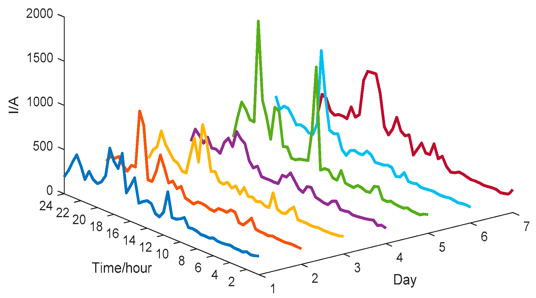
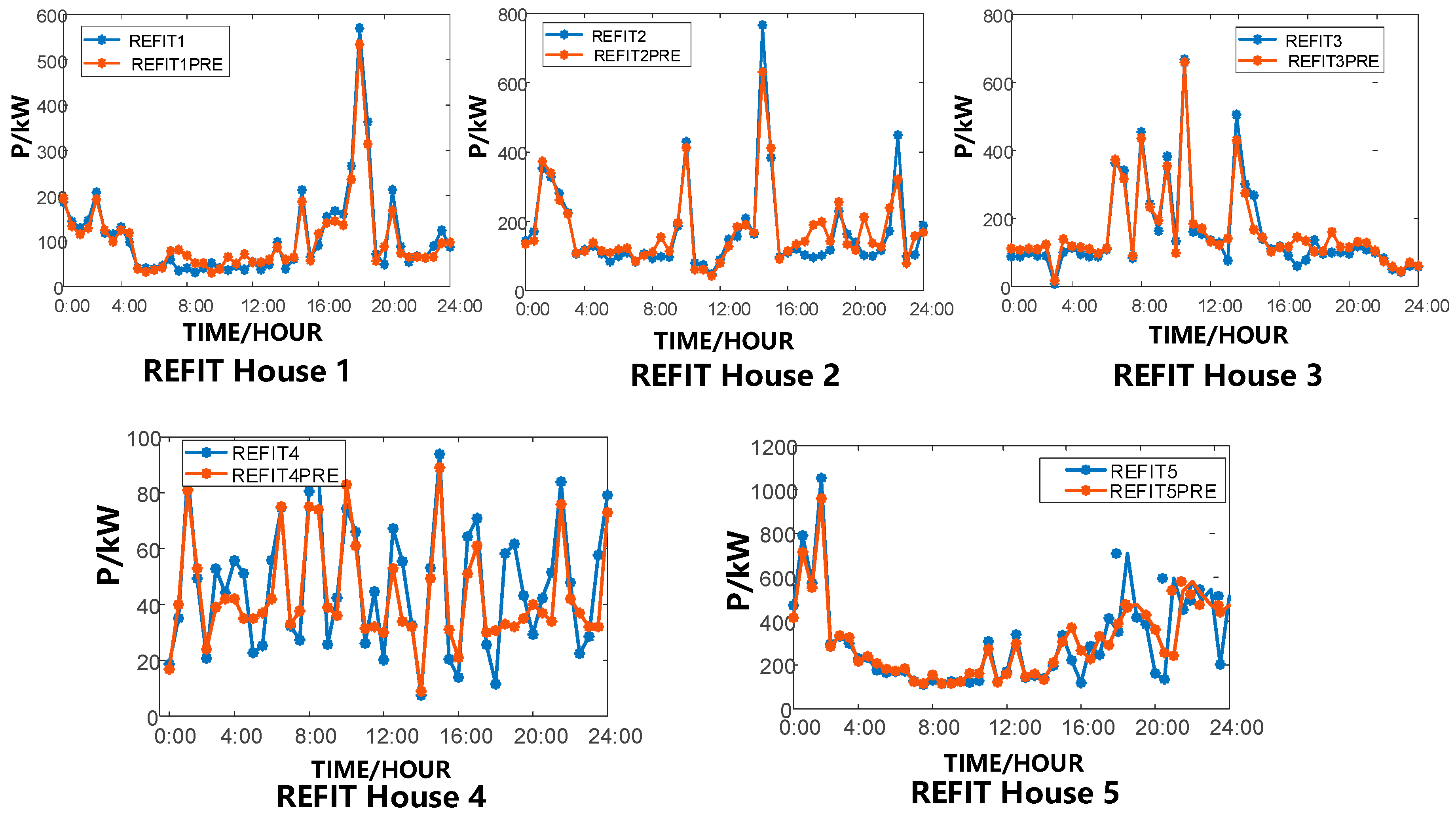
4.1. Description of The Dataset

The data used to verify the validity of the proposed method were obtained from AMPds dataset and REFIT dataset. AMPds dataset comprehensively records the minutely current readings of a Canadian household and its 19 appliances for 730 days. The data was collected from a house in the Greater Vancouver metropolitan area in British Columbia (Canada) and has been cleaned to provide for consistent and comparable accuracy results amongst different researchers and machine learning algorithms. The house has one level above grade and a basement making up a total of 199 m2. The main floor ceiling height is 2.44 m and the basement ceiling height is 2.13 m. The house has a family of three persons: A male and a female adult in their late 30 s and a daughter between the age of 5 and 6. The male adult is a full-time student at a local university, the female adult is self-employed, and the child attends full-time elementary school [33]. The minutely electricity consumption in the original dataset has been converted to consumption for every 30 min to match the common measurement frequency of existing smart meters and to obtain realistic results. Therefore, the original load matrix is 48 × 730.
This study selected the load profiles of three representative household appliances (heat pump, cloth washer and television) obtained from submetering for four random weeks to create the initial dictionary, which was a 48 × 84 matrix. The test experiment was implemented on Matlab and Python platforms.

4.2. Test Cases and Results

To assess the performance of the proposed method in short-term household load demand estimation, four widely used criteria were employed [20], including compress ratio (CR), mean absolute percent error (MAPE), mean absolute error (MAE) and root mean squared error (RMSE).
C R = s 0 N
R M S E = 1 N M i = 1 M ( y i j = 1 J x j d j ) 2
M A E = 1 N M i = 1 M | y i j = 1 J x j d j |
M A P E = 1 N i = 1 N | y i ^ y i y i ^ | 100 %
where y i ^ denotes the actual consumption data and y i denotes the estimation values at time index i.
This assessment consisted of three parts: (1) The effect of adding appliance status to the initial dictionary was determined by comparing between the proposed K-SVD algorithm with appliance status and the normal K-SVD algorithm; (2) the effect of increasing learning depth was demonstrated to show the potential of deep learning for short-term load demand estimation and the challenge of overfitting; (3) the performance of the proposed method was compared with ARIMA, MLP, LSTM, LSTM with normal and deep K-SVD and algorithm proposed in [23] to validate the efficacy.

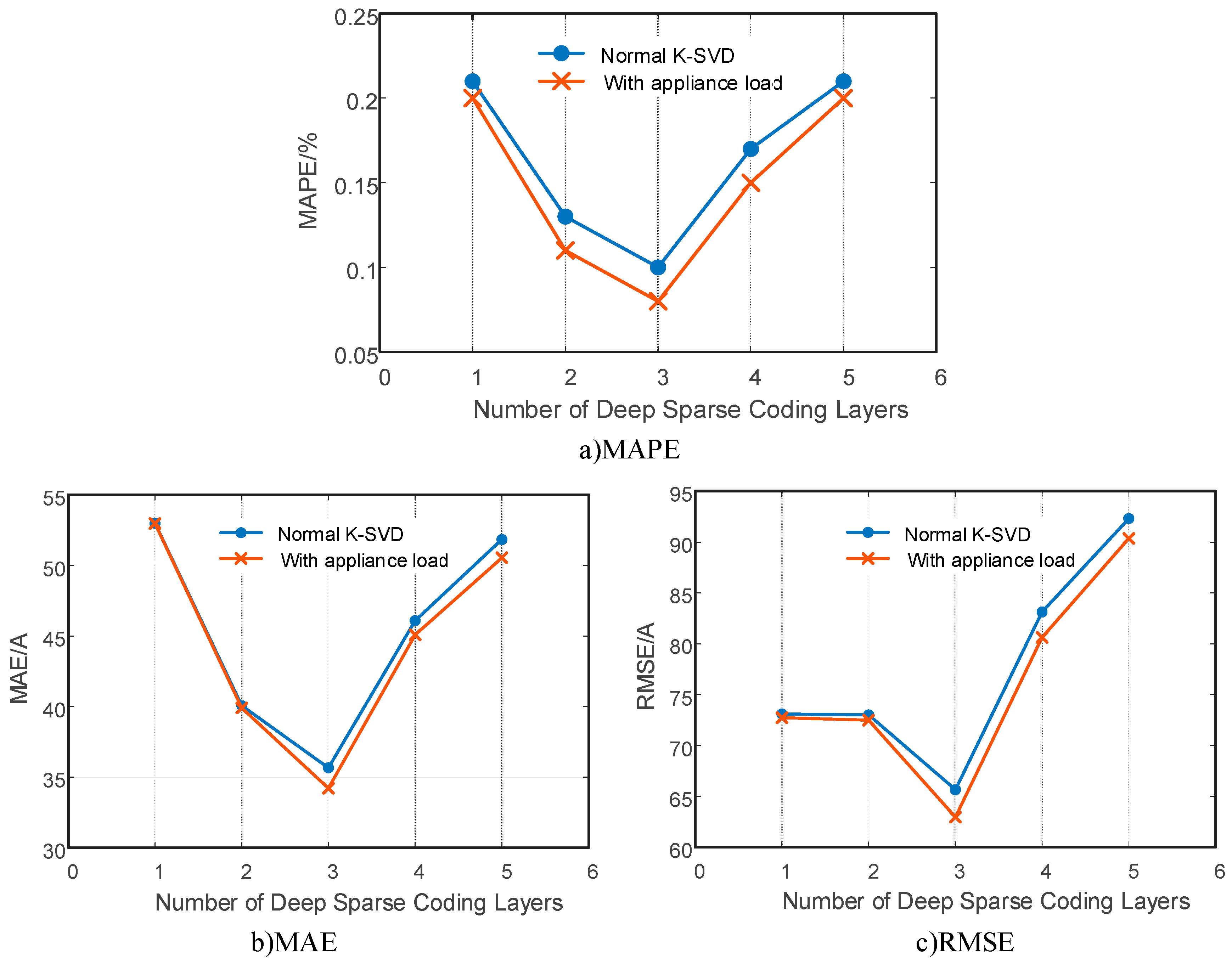
4.2.1. Effect of Adding Appliance Status into the Initial Dictionary

Figure 7 shows the electricity consumption of a family on a random week (24–30 June 2013). The load began to increase at 06:00, achieved a small peak at approximately 08:00, and typically reached the peak for one day at 18:00–20:00. The load profiles were consistent with the daily living habits of residents. For example, the washing and breakfast time of citizens was at 08:00 after getting up at 06:00. Upon returning home at 18:00, residents may take a bath, cook dinner, or engage in some form of entertainment. These activities considerably impacted the load profile and exhibited certain regularity.
Using the appliance load as the initial dictionary of the K-SVD algorithm tended to make the extracted DUBPs consistent with customer behavior and ensured sparsity. To achieve a fair assessment, sparse coding with and without appliance load scenarios were performed 100 times with the number of iterations K = 60.
Table 1 compares the performance of the proposed edge deep K-SVD algorithm with appliance load data with the traditional deep K-SVD algorithm. Notably, MAPE of the 3-layer K-SVD algorithm was already small, so the improvement was not obvious. However, as illustrated, the proposed algorithm maintained a significant improvement in RMSE and MAE in all three tested compression ratios.

4.2.2. Effect from Shallow to Deep

A sensitivity analysis was conducted to systematically evaluate the effect of learning depth on sparse coding. The edge deep K-SVD algorithms with different depths were: (1) Subjected to the same input size, output size, and iteration configuration parameters; (2) set to s 0 = 5 to limit the non-zero elements of the coefficient vector to five, and five DUBPs were extracted from the original AMI data; and (3) the averaged values of 20 tests were obtained. The results are presented in Figure 8.
As shown in Figure 8, the proposed deep K-SVD algorithm received an obvious improvement from layer 1 to layer 2. From layer 2 to layer 3, the improvement was nominal and deep K-SVD witnessed the best performance with 3 layers, with approximately 0.08% in MAPE, 34.22 A in MAE, and 62.96 A in RMSE. Further increases in learning depth did not improve the results and the reconstruction precision reduced as the learning went deeper because of the overfitting issue.

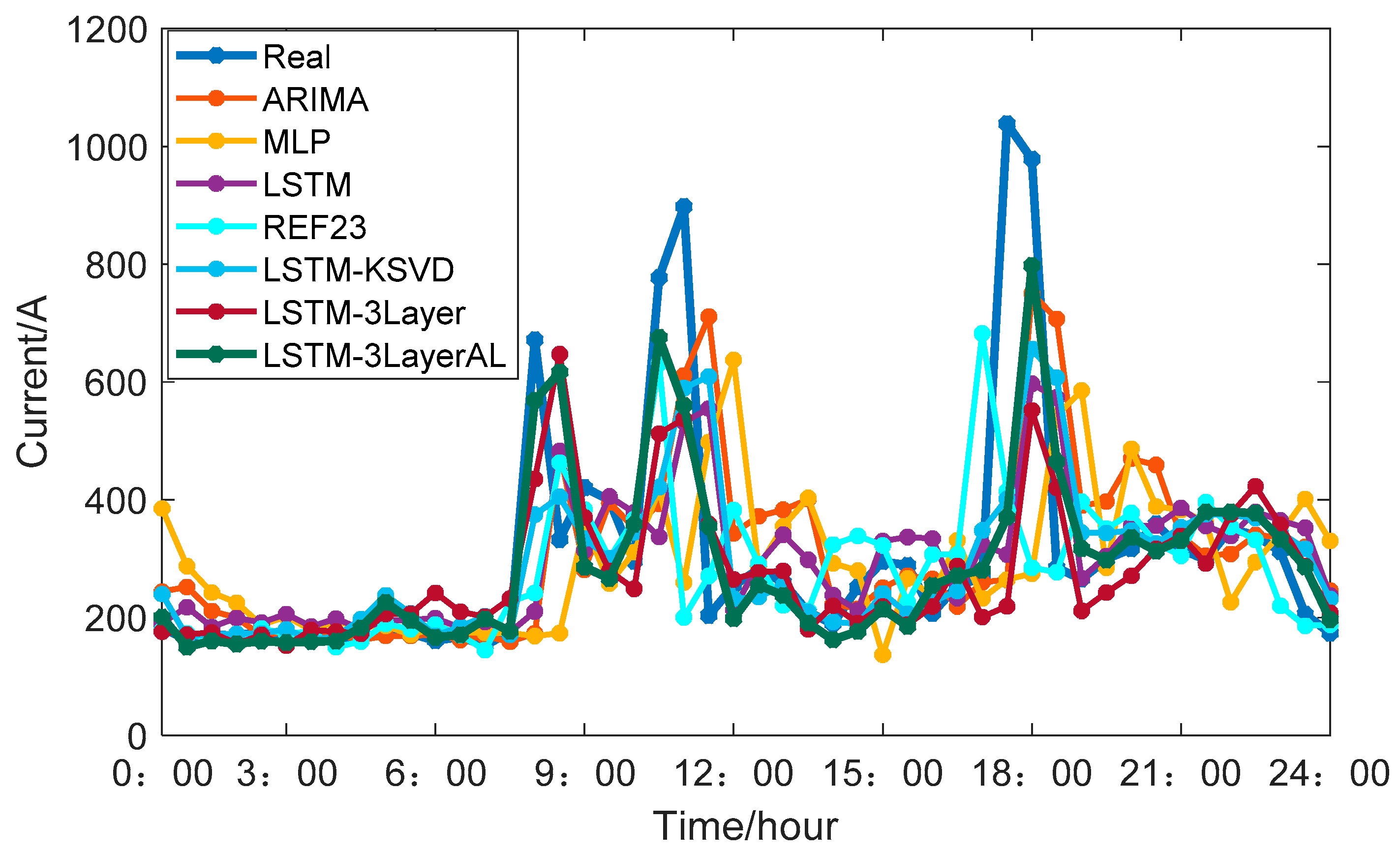
4.2.3. Benchmarking of Load Demand Estimation Methods in Households

To validate the effectiveness of the proposed two-stage estimation approach for household electricity demand, this study selected five other load demand forecasting methods for comparison under the preceding benchmarks. These methods are ARIMA, MLP, LSTM, LSTM with normal K-SVD, LSTM with 3-layer K-SVD and the forecasting algorithm proposed in [23].
The performance of the proposed two-stage LSTM with 3-layer appliance load based the K-SVD method and the five competitive techniques in terms of MAPE, MAE, and RMSE is provided in Table 2. For the testing sample, LSTM with 3-layer K-SVD outperformed ARIMA, MLP, normal LSTM, and LSTM with shallow K-SVD in all the metrics used. The novel electricity demand estimation method can further improve its performance with the introduction of appliance status into K-SVD coding. In particular, the proposed method resulted in 16.4%, 11.38%, and 18.16% reduction in MAE, MAPE, and RMSE, respectively, compared with LSTM with shallow K-SVD. Meanwhile, the improvement in MAE, MAPE, and RMSE using the proposed method reached 15.64%, 21.12%, and 25.37%, respectively, compared with algorithm proposed in [23].
Figure 9 presents the actual and forecasted load profiles using different methods on a random day. It was noted that currents estimated by the proposed method or other available forecasting methods were not completely consistent with the real currents, especially for higher values. It was mainly caused by the high randomness, volatility and uncertainty of load profiles at the household level and more sensitive to consumer behavior or environmental variables. Although the errors cannot be eliminated, the proposed algorithm made great progress and followed the trend of the actual load curve compared with the existing algorithms. The electricity consumption peak at approximately 08:00 and 11:30 was accurately captured, and overprediction of the peak at 09:15 and 13:00 due to inertia was avoided.
This study selected five peak periods during a day (08:00, 10:00, 11:00, 17:30, and 18:00) to calculate the absolute error between the predicted and actual loads. Figure 10 illustrates that LSTM with shallow K-SVD inaccurately estimated the highest peak of electricity consumption throughout the day (08:00) with an error of 508 A, whereas the error of the proposed two-stage LSTM with 3-layer appliance load based on K-SVD remained below 90 A. Figure 10 shows that our novel estimation approach was more stable in nearly all peak periods, thereby establishing that the DUBPs acquired using edge deep K-SVD coding with appliance load improved the estimation accuracy of ultra-short term residential electricity demand.
In order to verify the universality of the proposed method, this study selected five households with different load patterns and different consumption magnitude in REFIT to operate the experiment [34]. Sociodemographic information and other relevant information of each house is shown in Table 3. Experiment results are shown in Figure 11 and Table 3 and illustrated the proposed method can also achieve significant performance in all five houses.

5. Conclusions

A novel two-stage estimation approach for household electricity demand based on edge deep sparse coding was proposed to improve the estimation accuracy of ultra-short term residential electricity demand. The deep non-negative sparse coding algorithm was implemented in the sparse coding stage to extract usage patterns. The initial matrix contained the usage state of household devices. DUBPs were used as input to the LSTM network in the forecasting stage.
The results of the test experiments demonstrated that the proposed method can achieve considerable improvement in household-level consumption demand estimation and can substantially improve its performance at peaks and troughs. In terms of MAPE, the proposed method outperformed MLP by 51.26%, ARIMA by 36.62%, and LSTM with shallow K-SVD by 16.4%. In the field of mean absolute error and root mean squared error, the improvement was 53.95% and 36.73% compared with MLP, 28.47% and 23.36% compared with ARIMA, 11.38% and 18.16% compared with LSTM with shallow K-SVD.
Future work can focus on improving the estimation accuracy in two aspects. One is to continue exploring the hidden information of the household load or electrical equipment load to extract more effective behavior patterns. The other is to further utilize the potential of the proposed deep learning network by solving the overfitting issue of deep learning or adding other external factors, such as temperature, relative humidity, and their higher-order terms and interactions to establish a deep learning model that is more suitable for household load prediction.

Author Contributions

Conceptualization, Y.L., Y.S. and B.L.; formal analysis, Y.L. and B.L.; writing-original draft, Y.L.; writing-review & editing, Y.L., Y.S. and B.L.

Funding

This work was funded by National Natural Science Foundation of China (Grant No. 51777068) and Fundamental Research Funds for the Central Universities (Grant No. 2019QN110).

Conflicts of Interest

The authors declare no conflicts of interest.

References

  1. Saputro, N.; Akkaya, K.; Uludag, S. A survey of routing protocols for smart grid communications. Comput. Netw. 2012, 56, 2742–2771. [Google Scholar] [CrossRef]
  2. Peppanen, J.; Reno, M.J.; Thakkar, M.; Grijalva, S.; Harley, R.G. Leveraging AMI Data for Distribution System Model Calibration and Situational Awareness. IEEE Trans. Smart Grid 2015, 6, 2050–2059. [Google Scholar] [CrossRef]
  3. Godina, R.; Rodrigues, E.M.G.; Pouresmaeil, E.; Matias, J.C.O.; Catalao, J.P.S. Model Predictive Control Home Energy Management and Optimization Strategy with Demand Response. Appl. Sci. 2018, 8, 408. [Google Scholar] [CrossRef]
  4. Kwac, J.; Flora, J.; Rajagopal, R. Household Energy Consumption Segmentation Using Hourly Data. IEEE Trans. Smart Grid 2014, 5, 420–430. [Google Scholar] [CrossRef]
  5. Mahmoudi-Kohan, N.; Moghaddam, M.P.; Sheikh-El-Eslami, M.K.; Shayesteh, E. A three-stage strategy for optimal price offering by a retailer based on clustering techniques. Int. J. Electr. Power Energy Syst. 2010, 32, 1135–1142. [Google Scholar] [CrossRef]
  6. Rhodes, J.D.; Cole, W.J.; Upshaw, C.R.; Edgar, T.F.; Webber, M.E. Clustering analysis of residential electricity demand profiles. Appl. Energy 2014, 135, 461–471. [Google Scholar] [CrossRef] [Green Version]
  7. Sun, G.; Cong, Y.; Hou, D.; Fan, H.; Xu, X.; Yu, H. Joint Household Characteristic Prediction via Smart Meter Data. IEEE Trans. Smart Grid 2017, 10, 1834–1844. [Google Scholar] [CrossRef] [Green Version]
  8. Wang, Y.; Gan, D.; Sun, M.; Zhang, N.; Lu, Z.; Kang, C. Probabilistic individual load forecasting using pinball loss guided LSTM. Appl. Energy 2019, 235, 10–20. [Google Scholar] [CrossRef]
  9. Ramchurn, S.; Vytelingum, P.; Rogers, A.; Jennings, N.R. Putting the “smarts” into the smart grid: A grand challenge for artificial intelligence. Commun. ACM 2012, 55, 86–97. [Google Scholar] [CrossRef]
  10. Zehir, M.A.; Batman, A.; Bagriyanik, M. Review and comparison of demand response options for more effective use of renewable energy at consumer level. Renew. Sustain. Energy Rev. 2016, 56, 631–642. [Google Scholar] [CrossRef]
  11. Zhou, K.-L.; Yang, S.-L.; Shen, C. A review of electric load classification in smart grid environment. Renew. Sustain. Energy Rev. 2013, 24, 103–110. [Google Scholar] [CrossRef]
  12. Notaristefano, A.; Chicco, G.; Piglione, F. Data size reduction with symbolic aggregate approximation for electrical load pattern grouping. IET Gener. Transm. Distrib. 2013, 7, 108–117. [Google Scholar] [CrossRef]
  13. Zordan, D.; Martinez, B.; Vilajosana, I.; Rossi, M. On the performance of lossy compression schemes for energy constrained sensor networking. ACM Trans. Sens. Netw. 2014, 11, 15. [Google Scholar] [CrossRef]
  14. Yu, C.-N.; Mirowski, P.; Ho, T.K. A Sparse Coding Approach to Household Electricity Demand Forecasting in Smart Grids. IEEE Trans. Smart Grid 2016, 8, 1–11. [Google Scholar] [CrossRef]
  15. Tong, X.; Kang, C.; Xia, Q. Smart Metering Load Data Compression Based on Load Feature Identification. IEEE Trans. Smart Grid 2016, 7, 1. [Google Scholar] [CrossRef]
  16. Tcheou, M.P.; Lovisolo, L.; Ribeiro, M.V.; Da Silva, E.A.; Rodrigues, M.A.; Romano, J.M.; Diniz, P.S. The compression of electric signal waveforms for smart grids: State of the art and future trends. IEEE Trans. Smart Grid 2013, 5, 291–302. [Google Scholar] [CrossRef]
  17. Mehra, R.; Bhatt, N.; Kazi, F.; Singh, N.M. Analysis of PCA based compression and denoising of smart grid data under normal and fault con-ditions. In Proceedings of the 2013 IEEE International Conference on Electronics, Computing and Communication Technologies, Bangalore, India, 17–19 January 2013; pp. 1–6. [Google Scholar]
  18. de Souza JC, S.; Assis TM, L.; Pal, B.C. Data compression in smart distribution systems via singular value decomposition. IEEE Trans. Smart Grid 2015, 8, 275–284. [Google Scholar] [CrossRef]
  19. Unterweger, A.; Engel, D. Resumable load data compression in smart grids. IEEE Trans. Smart Grid 2014, 6, 919–929. [Google Scholar] [CrossRef]
  20. Wang, Y.; Chen, Q.; Kang, C.; Xia, Q.; Luo, M. Sparse and redundant representation-based smart meter data compression and pattern extraction. IEEE Trans. Power Syst. 2016, 32, 2142–2151. [Google Scholar] [CrossRef]
  21. Ahmad, A.; Javaid, N.; Alrajeh, N.; Khan, Z.A.; Qasim, U.; Khan, A. A Modified Feature Selection and Artificial Neural Network-Based Day-Ahead Load Forecasting Model for a Smart Grid. Appl. Sci. 2015, 5, 1756–1772. [Google Scholar] [CrossRef]
  22. Xie, J.; Chen, Y.; Hong, T.; Laing, T.D. Relative humidity for load forecasting models. IEEE Trans. Smart Grid 2018, 9, 191–198. [Google Scholar] [CrossRef]
  23. Kong, W.; Dong, Z.Y.; Hill, D.J.; Luo, F.; Xu, Y. Short-term residential load forecasting based on resident behaviour learning. IEEE Trans. Power Syst. 2017, 3, 1087–1088. [Google Scholar] [CrossRef]
  24. Yu, C.-N.; Mirowski, P.; Ho, T.K. A sparse coding approach to household electricity demand estimation in smart grids. IEEE Trans. Smart Grid 2017, 8, 738–748. [Google Scholar]
  25. Quilumba, F.L.; Lee, W.-J.; Huang, H.; Wang, D.Y.; Szabados, R.L. Using smart meter data to improve the accuracy of intraday load forecasting considering customer behavior similarities. IEEE Trans. Smart Grid 2015, 6, 911–918. [Google Scholar] [CrossRef]
  26. Kong, W.; Dong, Z.Y.; Jia, Y.; Hill, D.J.; Xu, Y.; Zhang, Y. Short-term residential load forecasting based on LSTM recurrent neural network. IEEE Trans. Smart Grid 2019, 10, 841–851. [Google Scholar] [CrossRef]
  27. Wang, Y.; Chen, Q.; Hong, T.; Kang, C. Review of smart meter data analytics: Applications, methodologies, and challenges. IEEE Trans. Smart Grid 2019, 10, 3125–3148. [Google Scholar] [CrossRef]
  28. Bruckstein, A.M.; Aharon, M.; Elad, M. K-SVD and its non-negative variant for dictionary design. Opt. Photonics 2005, 5914, 591411. [Google Scholar]
  29. Tariyal, S.; Majumdar, A.; Singh, R.; Vatsa, M. Deep dictionary learning. IEEE Access 2016, 4, 10096–10109. [Google Scholar] [CrossRef]
  30. Bhotto, M.Z.A.; Makonin, S.; Bajić, I.V. Load disaggregation based on aided linear integer programming. IEEE Trans. Circuits Syst. II Express Briefs 2017, 64, 792–796. [Google Scholar] [CrossRef]
  31. Shi, W.; Cao, J.; Zhang, Q.; Li, Y.; Xu, L. Edge Computing: Vision and Challenges. IEEE Internet Things J. 2016, 3, 1. [Google Scholar] [CrossRef]
  32. Graves, A.; Schmidhuber, J. Framewise phoneme classification with bidirectional LSTM and other neural network architectures. Neural Netw. 2005, 18, 602–610. [Google Scholar] [CrossRef] [PubMed]
  33. Makonin, S.; Popowich, F.; Bartram, L.; Gill, B.; Bajić, I.V. AMPds: A Public Dataset for Load Disaggregation and Eco-Feedback Research. In Proceedings of the 2013 IEEE Electrical Power & Energy Conference, Halifax, NS, Canada, 21–23 August 2013; Wadsworth: Belmont, CA, USA, 1993; pp. 123–135. [Google Scholar]
  34. REFIT: Personalised Retrofit Decision Support Tools for UK Homes Using Smart Home Technology. Available online: http://www.refitsmarthomes.org/index.php/refit-launches (accessed on 26 June 2019).
Figure 1. Schematic diagram of sparse coding.
Information 10 00224 g001
Figure 2. Schematic diagram of deep equipment behavior patterns extraction.
Information 10 00224 g002
Figure 3. Deep non-negative K-SVD algorithms with an appliance load.
Information 10 00224 g003
Figure 4. The edge sparse coding architecture for load data.
Information 10 00224 g004
Figure 5. The structure of memory cell in LSTM.
Information 10 00224 g005
Figure 6. Flowchart of proposed two-stage household electricity demand estimation approach.
Information 10 00224 g006
Figure 7. Daily load profiles of a single residential customer for one week.
Information 10 00224 g007
Figure 8. Reconstruction performance sensitivity investigation regarding the number of deep sparse coding layers: (a) MAPE, (b) MAE, (c) RMSE.
Information 10 00224 g008
Figure 9. Forecasting results throughout a day for the leading scenarios using data from AMPds dataset.
Information 10 00224 g009
Figure 10. Absolute error at peak hours of the leading algorithms.
Information 10 00224 g010
Figure 11. Actual (blue) and forecasted load profiles (red) throughout a day for the leading scenarios in five households from REFIT dataset.
Information 10 00224 g011
Table 1. Reconstruction performance comparison with different sparse coding algorithms.
CRAlgorithmRMSE (A)MAE (A)MAPE (%)
0.12503-layer K-SVD57.3731.770.07%
3-layer K-SVD with appliance load54.7430.070.06%
0.10423-layer K-SVD65.6635.670.10%
3-layer K-SVD with appliance load62.9633.220.08%
0.08333-layer K-SVD71.7439.040.14%
3-layer K-SVD with appliance load69.4937.730.13%
Table 2. Forecasting performance comparison between proposed method and existing algorithms.
AlgorithmMAPE (%)MAE (A)RMSE (A)
ARIMA31.84%109.63192.80
MLP41.41%143.49233.54
LSTM27.62%100.51180.55
Ref. [23]23.92%99.42198.00
LSTM-KSVD (with normal K-SVD)24.14%88.50167.28
LSTM-3Layer (with 3-layer K-SVD)22.67%87.71157.07
LSTM-3LayerAL
(with 3-layer appliance load based K-SVD)
20.18%78.42147.76
Improvement from LSTM-KSVD to LSTM-3LayerAL16.4%11.38%18.16%
Improvement from ARIMA to LSTM-3LayerAL36.62%28.47%23.36%
Improvement from MLP to LSTM-3LayerAL51.26%53.95%36.73%
Table 3. Forecasting performance in five houses of REFIT using the proposed method.
REFITSociodemographic InformationRMSE (kW)MAE (kW)MAPE (%)
REFIT House12 people
3 bedrooms
27 equipment
21.3017.2724.14%
REFIT House22 people
4 bedrooms
33 equipment
43.2628.8420.58%
REFIT House33 people
3 bedrooms
26 equipment
31.7522.6622.79%
REFIT House41 people
3 bedrooms
19 equipment
11.879.7426.53%
REFIT House54 people
4 bedrooms
44 equipment
93.2157.2621.76%

