Article

Liver Cancer Classification Model Using Hybrid Feature Selection Based on Class-Dependent Technique for the Central Region of Thailand

by
Rattanawadee Panthong
* and
Anongnart Srivihok
Computer Science Department, Faculty of Science, Kasetsart University, 50 Ngam Wong Wan Rd., Bangkok 10900, Thailand
*
Author to whom correspondence should be addressed.
Information 2019, 10(6), 187; https://doi.org/10.3390/info10060187
Submission received: 23 April 2019 / Revised: 24 May 2019 / Accepted: 29 May 2019 / Published: 31 May 2019
(This article belongs to the Section Artificial Intelligence)

Abstract

:
Liver cancer data always consist of a large number of multidimensional datasets. A dataset that has huge features and multiple classes may be irrelevant to the pattern classification in machine learning. Hence, feature selection improves the performance of the classification model to achieve maximum classification accuracy. The aims of the present study were to find the best feature subset and to evaluate the classification performance of the predictive model. This paper proposed a hybrid feature selection approach by combining information gain and sequential forward selection based on the class-dependent technique (IGSFS-CD) for the liver cancer classification model. Two different classifiers (decision tree and naïve Bayes) were used to evaluate feature subsets. The liver cancer datasets were obtained from the Cancer Hospital Thailand database. Three ensemble methods (ensemble classifiers, bagging, and AdaBoost) were applied to improve the performance of classification. The IGSFS-CD method provided good accuracy of 78.36% (sensitivity 0.7841 and specificity 0.9159) on LC_dataset-1. In addition, LC_dataset II delivered the best performance with an accuracy of 84.82% (sensitivity 0.8481 and specificity 0.9437). The IGSFS-CD method achieved better classification performance compared to the class-independent method. Furthermore, the best feature subset selection could help reduce the complexity of the predictive model.

1. Introduction

Liver cancer is the major cause of cancer death in Thailand; its mortality there is higher in males and old people [1]; it was ranked the second top cancer incidence in Thailand [2]. This work focuses on the classification of Hepatocellular Carcinoma (HCC). HCC is the fifth most common tumor worldwide and the second leading cause of cancer deaths, with persistently increasing mortality in Southeast Asia and Thailand [3,4]. It is the most common type of liver cancer. HCC is a primary malignancy of the liver and occurs predominantly in patients with underlying chronic liver disease and cirrhosis [3,4]. Furthermore, most cases of HCC are associated with the hepatitis B virus, hepatitis C virus infection, alcohol-induced cirrhosis, or other chemical carcinogens [3,5]. The tumor-node-metastasis (TNM) staging system is used for cancer staging all over the world. It is important for doctors to use the same staging system. The TNM system assesses primary tumor features (T), the presence or absence of nodal involvement (N), and distant metastasis (M) [6,7].
Feature selection is a technique of choosing a subset of variables from the original data. The main benefits of performing feature selection before modeling consist of reducing overfitting, improving the classification accuracy and reducing the training time. Feature selection and classification methods are of particular interest in high-dimensional and multiple-class datasets [8]. Furthermore, classification problems occurring in practice involve large datasets with many features and multiple classes, namely bioinformatics, multimedia and microarray data [8,9]. If a dataset consists of many features and multi-class datasets, the irrelevant attributes will impact on the design of the classification model, and classification accuracy may be decreased. Therefore, feature selection can serve as a preprocessing tool of great importance in solving classification problems. Furthermore, it can help to remove irrelevant and redundant features by increasing the accuracy of classification models [10].
Feature selection plays a vital role in classification problems by reducing the complexity of a classifier and reducing the overall cost of feature measurements. The feature selection approaches were classified into three categories: filters, wrappers, and the embedded method [9]. The filter methods involve selected features based upon some predefined criteria such as correlation criteria or mutual information [10]. The filter techniques construct a rank of features [11]. These methods select features based on discriminating criteria that are feature subsets independent of classification [12]. Filters generally involve a non-iterative computation on the dataset since filters evaluate the intrinsic properties of the data without using a classifier and tend to select large subsets [12]. Wrapper methods perform feature selection by making use of the classifier to evaluate the feature subset. These methods perform the feature selection by making use of a specific classification model [11,13]. The wrappers have a mechanism to avoid overfitting, because these methods use cross validation measures of predictive accuracy [14]. Although the wrapper method achieves better accuracy rates than a filter approach, this method increases the computational cost. Embedded methods are similar to wrapper algorithms, since they are performed subset feature selection by machine learning models for classification. In embedded methods, the feature selection algorithm is integrated as part of the learning procedure. Also, these approaches are used for mathematical optimization [15]. The examples of this approach are support vector machine based on recursive feature elimination (SVM-RFE) and the LASSO algorithm [9].
In summary, the benefit of the filter method is its rapid calculation; this method is often applied to feature selection in high-dimensional data, whereas the advantages of the wrapper method are improved for accuracy. A hybrid method involves the combination of filter and wrapper-based methods. It is very helpful in improving computational speed and prediction accuracy [16,17]. In the previous work [18], we used wrapper methods based on the ensemble learning method (involving the bagging and AdaBoost techniques) in UCI datasets. Three wrapper approaches (sequential forward selection, sequential backward selection (SBS), and optimized selection (evolutionary)) were used to select the feature subset from the original datasets. The experimental results indicate that sequential forward selection (SFS) with the ensemble learning algorithm provided good classification accuracy. However, the wrapper approaches increased the computational cost. Hence, in the present study, we employed the hybrid feature selection method to gain the best feature set and to improve accuracy and reduce complexity in the prediction model.
Recently, feature selection based on class-dependent criteria has received more attention because of the large amount of research in machine learning. Class-dependent feature selection in multi-class classification problems selects a set of unique features that use the discriminative power of each class. It provides a different feature subset for each class. In addition, the classification based on class-dependent feature subsets can help decrease overfitting. Overfitting occurs when the classification model or the trained learning algorithm fits the data too well; this leads to poor predictions with new samples. The results of the research in this field indicated that class-dependent feature selection is superior to class-independent feature selection [19]. From these research studies, we found few examples of class-dependent features in multi-class problems, specifically with regard to the classification of cancer datasets. Most feature selection and classification algorithms usually choose the optimal feature subset for all classes using the class independent technique. This is another key challenge in the multi-class classification problem. The features should be designed to represent subsets of classes that display specific properties without regard to other classes since the value of any class may be meaningless or irrelevant [20]. Therefore, the present work applied the concept of class-dependent feature selection with a hybrid feature selection method. In addition, we used the class-dependent feature selection method to identify unique features related to each stage disease (class) from the liver cancer datasets.
In the present work, we propose a method of hybrid feature selection based on the class-dependent technique for a liver cancer classification model using data form the central region of Thailand. The hybrid method (called IGSFS-CD) combines information gain (IG) as a filter approach and the SFS as a wrapper approach based on class-dependent features. The IGSFS-CD method focuses on multi-class classification. The liver cancer datasets for the experiment were from the Cancer Hospital Thailand database for the 11-year period from 2007 to 2017. Additionally, we improve the efficiency of the classification model using three ensemble learning methods, namely ensemble classifiers, bagging, and AdaBoost that can help reduce the variance and/or bias of a set of classifiers. All datasets were tested through 10-fold cross validation. Performance is measured based on accuracy sensitivity and specificity. This paper is organized as follows: Section 2 provides a review of the literature on hybrid feature selection based on the class-dependent technique. Section 3 presents our method. Section 4 describes the experiments and results. Section 5 analyzes the experimental results and provides their discussion. Finally, the conclusion and future work are presented in Section 6.

2. Background and Related Work

2.1. TNM Classification for Hepatocellular Carcinoma

The TNM staging system was developed by the American Joint Committee on Cancer (AJCC) and the Union for International Cancer Control (UICC) [6]. TNM is globally used as a tool for describing the amount and spread of cancer in a patient’s body [7]. It can be used to classify most types of cancer. T refers to the size and extent of the primary tumor; N describes the spread of cancer to nearby lymph nodes; and M refers to whether cancer has metastasized from the primary tumor to other parts of the body [6].

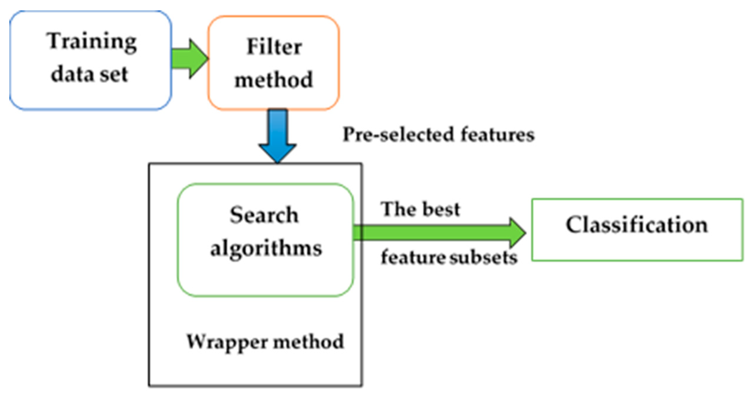
2.2. Hybrid Feature Selection Method

Many filter methods use preprocessing to rank the features. Filter algorithms are appropriate and effective approaches to deal with very high-dimensional datasets, are simple and fast regarding computational time, and are independent of the learning algorithm [9]. By contrast, wrapper methods depend on a classifier to obtain better accuracy, but this increases the time for preprocessing [21]. A hybrid of filter and wrapper techniques includes a filter to remove redundant and irrelevant features and uses the wrapper to evaluate a feature subset [22]. In summary, the hybrid method features the advantages of both the filters and the wrappers. It is applied to remove irrelevant and redundant attributes, to find the best feature subset, and to increase accuracy. The method of hybrid feature selection is shown in Figure 1.

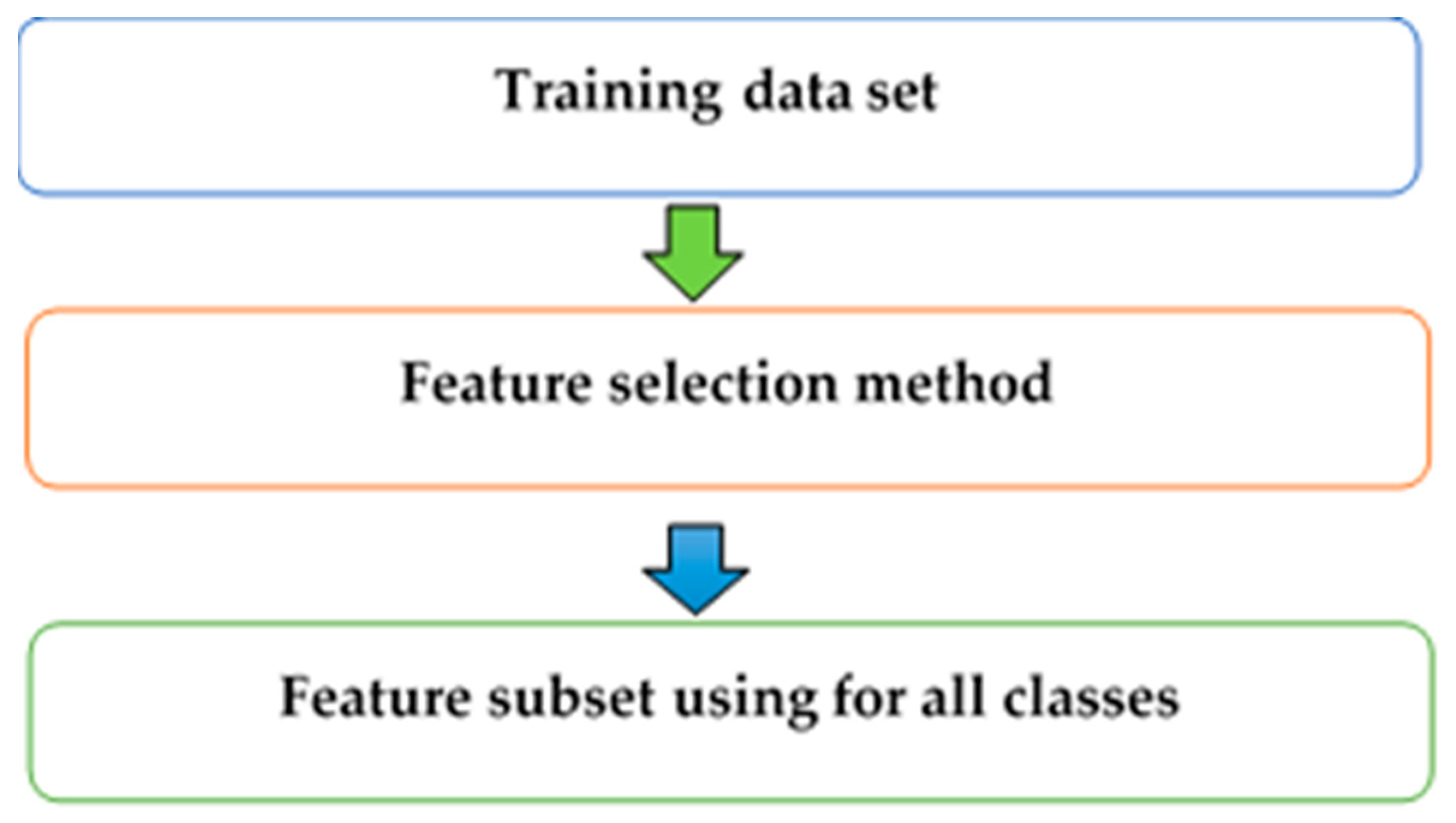
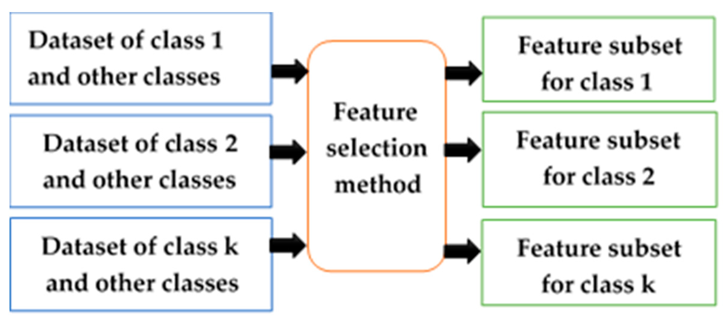
2.3. Class-Dependent and Class-Independent Techniques

The class-dependent (CD) technique is a method that chooses a unique feature subset for liver cancer in each stage (class). The attributes that depend on classes may have different feature subsets because each class has discrimination in terms of classifying. On the other hand, the class-independent (CID) technique is a method that chooses the same feature subset for all classes in the classification [23,24]. CD features in a many-class classification problem are features whose discrimination ability varies significantly depending on the classes [20]. Consequently, the CD feature selection can improve predictive accuracy and reduce the cost of feature measurement, compared with using the CID feature selection method. The CID technique is shown in Figure 2, and the CD technique is illustrated in Figure 3.

2.4. Classification for Multi-Class Problem

Multi-class classification problems challenge many traditional classifiers to select a set of characterizing features, and the targets of multi-class classification have more than two classes and impose more intricate tasks on multi-class classification problems. The approaches for multiple class classification problems are to transform the multiple class problems into several binary problems and then use a binary class learner for classification. Decomposing into binary classifications for multi-class pattern classification can apply the well-known One-versus-All (OVA) and One- versus -One (OVO) approaches. The OVA approach has been used to reduce the problem of classifying k classes into k binary problems, where each problem discriminates a given class from the other k−1 classes [25]. The OVO strategy is trained to distinguish the samples of one class from the samples of all remaining classes. It performs k (k −1) / 2 individual binary classifiers to evaluate all possible pairwise classifiers and combine binary classifiers through a majority vote [25]. When using the OVO approach with a dataset containing only a few instances, the classifier tends to be more prone to overfitting [26].

2.5. Related Work

This section reviews the hybrid feature selection method based on the CD technique for the cancer dataset. There are several novel combined methods involving filters and wrappers. Many researchers have proposed using hybrid feature selection for cancer datasets. For example, the hybrid feature selection for liver tissue pathological image classification which is called maximum minimum backward selection was proposed by Liu et al. [27]. This algorithm can obtain a good feature subset while achieving high accuracy classification in liver tissue pathological images. Consequently, the hybrid feature selection algorithm combines a filter algorithm and a wrapper algorithm, which results in rapid calculation by the filter algorithm and the high predictive accuracy by the wrapper algorithm. Gunasundari et al. [28] presented two types of hybridization, namely particle swarm optimization with sequential forward selection (PSO-SFS), and PSO with SFS and SBS (PSO-SFS-SBS) algorithms by combining the strengths of both the methods. MATLAB was used to classify liver disease as benign and malignant lesion from an abdominal CT. The hybrid feature selection approaches provided the very minimal best features using the probabilistic neural network (PNN) as classifier. The results of a hybrid PSO-SFS-SBS algorithm provided the best feature subset with 40% of features selected. Furthermore, the performance of classification gained the highest accuracy, i.e., 96.4 %, with 20 features for dataset-1 (85 features) and dataset-II (108 features) provides good accuracy, i.e., 92.6%, with 21 features [28]. Naqvi [22] presented a method involving a hybrid filter and wrapper. The filter used quadratic programing feature selection to remove redundant and irrelevant features, whereas the wrapper used SFS and SBS by combining the strengths of both methods. Furthermore, Hassan et al. [29] proposed ensemble filter methods using IG, gain ratio, symmetrical uncertainty, and SVM-RFE to rank all genes and selected the top genes. This method evaluates three datasets of gene expression, namely leukemia, lung cancer, and breast cancer with binary labels. Five classifiers were used to evaluate the selected features: decision trees (C4.5), support vector machines (SVM), random forest, K-nearest neighbors (KNN), and naïve Bayes (NB). The ensemble filter used bootstrapping (T = 10). Hassan reported that the accuracy of classification performance obtained by the proposed method was better than that by the other methods with all datasets. Ding et al. [30] proposed the similar method using IG and the sequential forward floating search with a DT. The optimal candidate feature subset is to rank using IG. The final optimal feature subset improved accuracy of classification and reduced maintaining iterations using the hybrid algorithm with the DT.
Other researchers have proposed a combination of feature selection techniques using IG as a filter method and binary PSO as a wrapper method in disease analysis and cancer diagnosis. The k-NN and SVM are used to evaluate the classification performance. The experimental results had higher predictive accuracy than other feature selection methods [31].
Recently, the hybrid feature selection method using the CD technique in multi-class problems has been of increased interest for machine learning. For example, hybrid methods for the F-statistic as a filter method were applied to preselect a small number of highly differentially expressed genes (features), and the maximum relevance binary particle swarm optimization (MRBPSO) and the class-dependent multi-category classification (CDMC) system as a wrapper-based method were proposed by Zhou et al. [19]. The MRBPSO and CDMC based on the CD technique were used to choose feature subsets for individual classes and to classify the samples. SVM and FKNN as classifiers with five-fold and Leave One Out cross validation accuracy as the evaluation criteria were used to evaluate the performance with the eight real cancer datasets. The experimental results indicated that the CD techniques increased accuracy compared to CID methods. In particularly, CDMC/SVM had an average accuracy of 99.9% in SRBCT dataset (the small round blue cell tumors of childhood), there are 2,308 features (genes). In addition, Nina Zhou et al. [32,33] presented developments to choose different feature subsets for different classes based on CD feature subsets in various biomedical datasets. The class separability measure was used as the rank feature, and SVM was used as the classifier. The Cleveland Heart Disease (13 features) and Ecoli datasets (7 features) were obtained from the UCI machine learning repository databases. The results showed that CD method produced better classification accuracies compared to those of the CID method in all datasets. These methods also can reduce data dimensionality. Moreover, each dataset was composed of several feature subsets to differentiate classes using SVM with 10-fold cross validation [32]. The structural similarity approaches for feature selection were based on CD. For example, the wrapper approaches that chose CD features in two artificial datasets and a variety of real-world benchmark datasets were proposed by Wang et al. [34]. These methods were measured using the RELIEF weight measure, class separability measure (CSM), and minimal-redundancy-maximal-relevance (mRMR) techniques, which helped remove irrelevant or redundant features and also improved the accuracy for classification. Wang et al. used the SVM as a classifier for the feature subset search algorithm. The one-against-one (OAO) strategy with the mRMR ranking measure was used to select CD features, and CD feature extraction used the one-against-all (OAA) strategy. The experimental results showed that the mRMR ranking measure provided better performance than the CSM ranking measure. In addition, the results using CD feature selection with the OAA strategy were better than those with the OAO strategy. In conclusion, the wrapper approach based on CD was superior to the filter method in terms of classification. Furthermore, Bailey [20] presented the CD features for the multi-class problem using a combination of feature extraction and feature selection. The method was divided into three classes by using a multi-layer perceptron and hierarchical classifier. The CD feature metric was used to select features for the submodels. The results showed the performance classification of CD feature using local feature selection was better than with global feature selection using a multi-layer perceptron and logistic linear discriminant classifiers for each submodel.

3. Materials and Methods

The framework of the present study includes three processes: data collection from the database of Cancer Hospital in Thailand, application of the preprocessing method for hybrid feature selection based on the CD technique to choose the best feature subset, and classification and evaluation using ensemble learning methods. The framework for hybrid feature selection based on the CD technique is shown in Figure 4. Furthermore, the names of the feature subset selection algorithms and associated abbreviations are given in Table 1.

3.1. Data Collection

In this experiment, both liver cancer datasets were acquired from Cancer Hospital Thailand database, also called Hospital Information System. The datasets were collected and stored in the MySQL database and then converted into a suitable format (a CSV file). LC_dataset-1 was retrieved from the MySQL database and consisted of cancer register dataset, public health minimum dataset and laboratory information system (LIS) for the 11-year period from 2007 to 2017. For LC_dataset-II consisted of a cancer register dataset, a public health minimum dataset, LIS, and nursing recorded data based on Gordon’s 11 functional health patterns for the 8-year period from 2010 to 2017. Gordon’s functional health patterns were as devised by Marjory Gordon for nursing assessment of patients [36,37].
In the present work, missing values estimation and discretization were used before applying the feature selection approaches. The missing categorical data was replaced by unknown value. In case of numerical features, the missing values were replaced by average value of each feature [38]. In addition, the unspecified class instances were removed. Then, numerical values in each feature were discretized by referencing value in the laboratory or user-defined values. Four different classes included stage 1, 2, 3, and 4 were assigned to the patients by domain expert medical doctors. The type of features consists of nominal and numeric. The characteristics of the datasets are shown in Table 2.

3.2. The Preprocessing Method for Class-Dependent Feature Selection

In the process of preprocessing, we presented a hybrid feature selection method. The scope of this work emphasized on the IG and the SFS techniques. The hybrid feature selection algorithm uses IG and SFS with two different classifiers (DT and NB).
IG is a feature-ranking method based on DTs that measure the amount of information in bits about the class prediction, if the only information available is the presence of a feature and the corresponding class distribution [39]. The IG is the main value for calculating the weight in each feature that uses the entropy metric to rank the features. It gives the entropy as a criterion of impurity in a training set. A smaller value of entropy is better. In this paper, we use weighting by IG to generate attribute weights. The IG is adopted to reduce the features in the first step. The concept of IG is to select features that reveal the most information about the classes [39]. The higher the weight of an attribute; the more relevant it is considered. The IG [35] is defined as
G a i ( S , A ) = E ( S ) v V a l u e s ( A ) | S v | | S | E ( S v )
where
E ( S ) = i = 1 n P i log 2 P i
i = 1 n P i log 2 P i = P 1 p log 2 P 1 p P 2 p log 2 P 2 p P n p log 2 P n p
SFS is the simplest greedy search algorithm [14]. The greedy search method is used to find the best subset. It adopts a bottom-up heuristic search criterion. SFS starts with an empty set or null set of attributes, and the remaining attributes and, in each round, it adds the most significant feature with respect to the set when combined with features that have already been selected [10,11]. To speed up the selection, a criterion is chosen that incrementally increases the objective function until the maximum is reached with the maximum number of features. Generally, related to performance, the criterion used is the accuracy of the learning machine performed [21]. Therefore, the attribute giving the highest increased accuracy is added to the selection. The SFS algorithm [40] is as follows:
  • Initialize the empty set Yk = {∅} at k = 0
  • Select the next best feature x to add to Yk with most significant cost reduction
  • Update Yk+1 = Yk + x; k = k + 1
  • Repeat step 2
The process of the preprocessing method contains four steps:
Step 1. The separation of each class using the OVA strategy: In this step, the OVA strategy including training a classifier per class for each classifier is applied. The datasets are transformed from multiple classes into several binary classes. The considered class sample is specified as class 1, and the rest is class 0.
Step 2. Hybrid feature selection method: Two types of feature selection tasks being used in this step included (were consisted of) the IG as a filter method and the SFS as a wrapper method. The filter technique reduces the number of variables. The IG algorithm uses the operator to select based on weights with the weight relation according to Top k. The k attributes with the highest weights are selected and k is specified by the k parameter. It is used to count the number of features to select. A higher weight value shows that the feature is more relevant to classification. The best configuration of parameter Top k is found by optimizing the parameters process using the RapidMiner software [41] based on trying from 10 to 35 approximately 20%–60% of all features in LC_dataset-1. In LC_dataset II the optimized parameter Top k is found by trying from 25 to 70 approximately 20–60% of all features. Subsequently, SFS is applied for subset selection undertaken from the subset using the wrapper method. A final subset is the best classifier accuracy from using learning algorithms.
Step 3. Subset evaluation: The feature subset evaluation is performed using two different classifiers (NB and DT). Each model is trained using different feature subsets. The performance of the different feature selector classifiers is calculated using 10-fold cross validation. A cross validation estimates the statistical performance of a learning algorithm by dividing data into separate training and test sets [42]. Moreover, it is used to measure the classification evaluation on the feature subset of each class and to compare the accuracy of the classification models.
Step 4. Integrated subset: The feature subsets are combined using the technique of relational algebra operators, namely union. A union approach can combine feature sets selected by each class which is used to discover the final feature subset. The classifier model is generated from the final feature subset.

3.3. Classifiers

In this work, three classifiers (NB, DT, and KNN) were used for the classification and evaluation models.
An NB classifier is a simple probabilistic classifier based on applying Bayes’ theorem, which can predict the class membership probabilities [43]. The NB model is easy to build and particularly useful for very large datasets due to f its simplicity and efficiency. The NB uses a classification algorithm for binary (two class) and multi-class classification problems. The performance of NB suffers in domains that involve correlated features. With many attributes, NB classifiers are especially attractive because of their efficiency [44]. The main advantage of the NB classifier is that it only requires a small amount of training data to estimate the means and variances of the variables necessary for classification.
A DT classifier is typically a top-down greedy approach, which provides a rapid and effective method for classifying data instances. It is easy to understand and explain. The DT method builds classification models in the form of a tree structure and is easy to update for new data [43,44]. Decision trees are generated by recursive partitioning and the recursion stops when all the examples or instances have the same label value. The tree-pruning technique of DT is used to remove noisy data and to improve the predictive model. The root node of DT is chosen based on the highest IG of the attribute [45]. The DT classifier provides a rapid and useful solution for classifying instances in large datasets with a large number of variables [43,45]. Classification using a DT has high accuracy, but its performance usually depends on the characteristics of the dataset [43].
KNN classification is a non-parametric supervised learning method and is also called a lazy learning algorithm. It is a type of instance-based learning [46]. The new instance will be assigned the point in a class among its KNN (k is number of neighbors and is a positive integer). If k = 5, then classification is by a majority vote (class label) of the five nearest points. In the present work, we used the Euclidean distance function to measure the distance metric. The Euclidean distance (d) is calculated as follows:
Let A and B be between two data points in the training dataset; the KNN classifier calculates the distance between A and B as
d ( A , B ) = ( x 1 x 2 ) 2 + ( y 1 y 2 ) 2
Furthermore, the configuration of optimized parameter k by RapidMiner software was k = 5.

3.4. Evaluation Model with Ensemble Learning Methods

Ensemble learning algorithms are sets of classifiers or training data in which multiple models are trained to solve the same problem. The ensemble methods use multiple classifiers or different training sets to obtain a more accurate classification [47]. In this work, three ensemble learning algorithms, namely ensemble classifiers (DT, NB, and KNN), bagging, and AdaBoost, were used for the assessment of the prediction model. Performance evaluation was performed through 10-fold cross validation, which is generally applied for classifying models and evaluation. The ensemble learning algorithms used multiple classifiers or different datasets to obtain a more accurate classification by combining many weak learners [47,48]. The ensemble approach for the classification problem is divided into two categories as follows:

3.4.1. Heterogeneous Classifiers Use the Same Data over Diversified Learning Algorithms

The learning procedure for ensemble algorithms is divided into two sections. The first section is construction of the base classifiers, and the second one is a voting task. The majority vote is the most popular approach. The vote is used to combine multiple classifiers [26,49].

3.4.2. Homogeneous Classifiers Use Different Data Sets with The Same Algorithm

Homogeneous classifiers are defined as ensembles, or sets, of training sets. This approach uses component classifiers of the same type. The base learners are trained by only one learning algorithm, the base learners are homogeneous. Two well-known ensemble methods are bagging [50] and boosting [51].
  • Bagging (bootstrap aggregating) is an ensemble method that creates different training sets by sampling with replacement from the original dataset on training individual classifiers [50,52]. It provides diversity in subsets that might reduce the variance of datasets and improve results of classification algorithms [53]. In this work, different training sets were obtained by resampling using bagging with a DT as the base classifier.
  • Boosting is an approach to machine learning that provides a highly accurate prediction rule by combining many relatively weak and inaccurate rules. The AdaBoost (adaptive boosting) algorithm was the first practical boosting algorithm [51]. AdaBoost is an algorithm for constructing a strong classifier as a linear combination of weak classifiers. It reduces the bias of multi-class datasets and it is applicable for building ensembles that empirically improve generalization performance [48,53]. In this work, the AdaBoost approach with DT as the base classifier is used to train datasets.

3.5. Performance Measures for Classification

In the present study, we used three evaluation measures, namely accuracy, sensitivity, and specificity.
Accuracy is classification performance measurement; the calculation of classification accuracy was measured using Equation (5).
( TP + TN ) ( TP + FN + FP + TN ) Accuracy = T P + T N T P + F N + F P + T N ,
where TP is the number of positive instances correctly classified, TN is the number of negative instances correctly classified, FN is the number of positive instances incorrectly classified as negative and FP is the number of negative instances incorrectly classified as positive [43].
Performance measures for multi-class classification use micro-average and macro-average methods. Macro-averaging computes the metric independently for each class and then takes the average, whereas micro-averaging aggregates the contributions of all classes to compute the average metric [54]. The macro-averaging approach can be used to treat all classes equally, whereas the micro-averaging approach can be used to measure datasets varying in size [54]. Thus, micro-averaging is suitable for a multi-class classification problem in imbalanced datasets (the number of instances of the one class is much higher than those of other classes) [54]. Table 3 demonstrates the confusion matrix applied in this work. The confusion elements for each class are given by:
Let k be the number of classes. Each element i, j of the matrix would be the number of items with true class i that were each classified as being in class j [55].
tpi = Cii
f n i   = l = 1 k C i l t p i
f p i = l = 1 k C l i t p i
t n i = l = 1 k n = 1 k C ln t p i f p i f n i
Sensitivity is the proportion of true positives that are correctly classified as positive class labels and is also called the true positive rate or the recall. It can be used to improve a classifier when there are more than two classes (multi-class problems) [56,57]. In the multi-class case, the sensitivity can be calculated as
Sensitivity micro   =   i = 1 k t p i i = 1 k ( t p i + f n i )
In this formula, the performance measure of the classifier is calculated using the sums of the individual true positives and false negatives of the k class.
Sensitivity macro   =   i = 1 k t p i ( t p i + f n i ) k
In this formula, the performance measure of the classifier is calculated from the average of the true positive rate of individual classes.
Specificity is the proportion of true negatives that are correctly classified as negative class labels, and this is also called the true negative rate [56]. In the multi-class case, the specificity can be computed as
Specificity micro   =   i = 1 k t n i i = 1 k ( t n i + f p i )
In this formula, the performance measure of the classifier is calculated from the sums of the individual true negatives and false positives of the k class;
Specificity macro   =   i = 1 k t n i ( t n i + f p i ) k
In this formula, the performance measure of the classifier is calculated from the average of the true negative rate of individual classes.
Furthermore, the present study used the RapidMiner studio version seven enterprise edition for model training and testing [41]. It was used as a tool for feature subset selection, training classifiers, and performance evaluation. The Python version 3.2 software (PyCharm Edu) with libraries imported from the Anaconda package was used to create class dependent feature selection.
Statistical tests have been used to test the performance measures. In statistics, the margin of errors (MOE) is an interval estimate, also called the confidence interval. It is a value computed from a variety of components [58]. In case the margin of error is low, the result is more reliable. Confidence intervals (CI) usually take the form:
  • CI = Point estimate ± Margin of error.
  • MOE = Critical value (z) × Standard error of point estimate
  • Standard   error = σ n
In the present study, the level of confidence is used at 95% to compare among different ensemble learning methods. The critical Z-score value is 1.96.

4. Results

In this section, the results of hybrid feature selection based on CD techniques for the liver cancer classification model were presented. The experimental results of the proposed method used the classification accuracy, sensitivity, and specificity of the two training sets of liver cancer datasets. The IGSFS-CD method was compared to common feature selection based on independent classes.

4.1. Performance of IGSFS-CD Approach Using Ensemble Learning Method On Lc_Dataset-1

From Table 4, the results of performance comparison concerning the accuracy of the LC_dataset-1, it indicated that IGSFS-CD in which DT was used to evaluate the subset had the highest average accuracy rate (76.98%) compared to the other methods. IGSFS-CID with NB had a higher average accuracy rate (76.73%) compared to the other class independent techniques. Although the accuracy of IGSFS-CD was lower than SFS-CD with DT by bagging learning algorithm, it was better than SFS-CD using NB-based methods. In addition, the accuracy of IGSFS-CD with DT using AdaBoost was equal to that of SFS-CID with NB by ensemble classifiers (78.36%), whereas our method using NB to evaluate the subset had a lower accuracy rate than of SFS-CID. The results, also, indicate that both IGSFS-CD and IGSFS-CID have similar performance on LC_dataset-1. The best result of IGSFS-CD with DT was obtained using the optimized parameters Top k = 25. In summary, the DT-based methods had better performance than the NB-based methods using AdaBoost algorithm.
The sensitivity and specificity values are illustrated in Table 5 and Table 6, respectively. From Table 5, it may be seen that IGSFS-CD with DT had good sensitivity performance except for IGSFS-CD using the bagging algorithm. The best performance of sensitivity values (Snµ = 0.7841 and SnM = 0.6047) were obtained using IGSFS-CD with DT in which the AdaBoost learning algorithm was used to classify the model. However, IGSFS-CD with NB was inferior to two class-independent methods (IGSFS-CID and SFS-CID). Moreover, the sensitivity values of IGSFS-CID with NB (Snµ = 0.7841 and SnM 0.6290) were better when ensemble classifiers were used.
The results from Table 6, it was clearly seen that the specificity values (Spµ = 0.9159 and SpM = 0.8609) of IGSFS-CD with DT using the AdaBoost learning algorithm were better than for all other methods except IGSFS-CID and SFS-CID. Furthermore, this approach provided specificity values higher than conventional class -independent methods using the bagging algorithm. However, IGSFS-CD with NB was inferior to two class-independent techniques (IGSFS-CID and SFS-CID).

4.2. Performance of the IGSFS-CD Approach by the Ensemble Learning Method on LC_dataset-II

The results based on the LC_dataset-II are shown in Table 7, Table 8 and Table 9. From Table 7, it may be seen that IGSFS-CD with NB had the best accuracy (84.82%) using ensemble classifiers compared to the common class methods. Furthermore, both IGSFS-CD and IGSFS-CID with NB using ensemble classifiers were superior to the other methods. However, the accuracy of IGSFS-CD with NB using bagging learning method was lower than compared to class-independent approaches. From Table 7, it may be seen that the performance of IGSFS-CD with DT achieved a high accuracy (83.39%) using ensemble classifiers compared to the class independent techniques. In addition, both IGSFS-CD and SFS-CD with DT had the highest average accuracy rate (79.22%) compared to the other methods. The best performance of IGSFS-CD with NB was obtained using the optimized parameters Top k = 50. In summary, NB-based methods had better performance than DT-based methods using ensemble classifiers.
Table 8 and Table 9 demonstrate the performance comparison for each method in terms of sensitivity and specificity, respectively. When considering the performances measured concerning sensitivity as shown in Table 8, it indicated that the best performance of IGSFS-CD with NB was as soon as it achieved the maximum sensitivity values (Snµ = 0.8481, SnM 0.7173) using ensemble classifiers. Furthermore, both IGSFS-CD and SFS-CD with DT-based methods given good sensitivity values using three ensemble leaning algorithms. Besides, it was obvious shown that two methods (IGSFS-CD and SFS-CD) have similar performance using DT as a classifier.
From Table 9, it may be seen that the specificity values of IGSFS-CD with NB using ensemble classifiers (Spµ = 0.9437 and SpM = 0.9273) were superior to the conventional class independent methods. Furthermore, results of this approach had good specificity which the AdaBoost was used to classify the model. However, specificity values of IGSFS-CD with NB were inferior to SFS-CD when the bagging was used as the learning algorithm. For IGSFS-CD with DT outperforms other methods using AdaBoost and bagging algorithms.

4.3. Selected Features by the Igsfs-Cd Approach

Table 10 shows that selected features of individual classes using the IGSFS-CD method on LC_dataset-1 and LC_dataset II. According to the selected features in Table 10, we found that the features (T) in the two datasets had the highest frequency (selected seven times from all classes). Furthermore, another attribute EXT was selected four times in the two datasets. Both features were most found in class 1 and class 4 of all datasets. Class labels represent all stages of liver cancer (stage 1–4). From Table 10, it may be seen that the number of selected features using the IGSFS-CD with DT was smaller than the IGSFS-CD with NB in two datasets. In addition, different classes had very distinguishing feature subsets when the NB classifier was used to evaluate subset of attributes.
The descriptions of each feature for the liver cancer datasets were presented in Tables S1 and S2 in supplementary materials. Tables S1 and S2 listed the final feature set from the IGSFS-CD method with subset evaluation DT and NB, respectively.

4.4. Estimation of Performance Measures

The estimation of accuracy, sensitivity, and specificity of performance measures are illustrated in Table 11 and Table 12. From Table 11, it may be seen that the IGSFS-CD method showed accuracy of 75.90 (95% CI 74.90 to 76.90), sensitivity of 0.6552 (0.5852 to 0.7252), and specificity of 0.8768 (0.8568; 0.8968) when the margin of errors is 0.01, 0.07, and 0.02 respectively. Furthermore, IGSFS-CD and IGSFS-CID methods demonstrated similar accuracy, sensitivity, and specificity.
Table 12 shows that IGSFS-CD method had the highest average accuracy at 77.86 (95% CI 73.86 to 81.86), sensitivity of 0.6808 (95% CI 0.6108 to 0.7508), and specificity of 0.8974 (95% CI 0.8774 to 0.9174) when the margin of errors is 0.04, 0.07, and 0.02 respectively.

5. Discussion

The overall performances of IGSFS-CD that improved the performance of the classification model using the liver cancer dataset are presented in this section. In the present study, we compared the performance of IGSFS-CD with that of three class independent methods (IG-CID, SFS-CID, and IGSFS-CID) and two class dependent methods (IG-CD and SFS-CD). The results indicated that IGSFS-CD using DT based methods had better performance than NB based methods with data LC_dataset-1. In contrast, the NB-based method had better performance than DT-based methods with the data LC_dataset II. IGSFS-CD with NB had the best performances with the LC_dataset-II using ensemble classifiers. In addition, IGSFS-CD with NB had good sensitivity and specificity values when ensemble classifiers were used as classifiers. The better performance could have been caused by two reasons. Firstly, IGSFS-CD can eliminate a feature that is irrelevant to the classification in machine learning. Secondly, IGSFS-CD can reduce the complexity of the model using the hybrid feature selection method. For instance, IGSFS-CD with DT predicted using the ensemble methods in the present study had the highest average accuracy with both datasets at 76.98% and 79.22%, respectively. The prediction performance of IGSFS-CD with NB is suitable for a domain with a large number of features (100 up) but relatively few instances. However, the effectiveness of IGSFS-CD with NB was inferior to class-independent methods with small numbers (less than 100) of features. IGSFS-CD with NB obtains the lower mean accuracy compared to CID methods for LC_dataset-1 due to the instances of classes having more unbalanced sample subsets than for LC_dataset-II. Although the accuracy using IGSFS-CD with NB was less than that from conventional methods for LC_dataset-1, IGSFS-CD with DT was effective when the AdaBoost algorithm was used. Therefore, our method might be a good alternative for a domain where there is a small number of samples but a large number of attributes. The classification performances of the hybrid feature selection methods were better than those of the single-feature selection methods. As with previous work [19], the hybrid filter and wrapper approaches based on CD feature selection methods were used to select a small subset of genes for each cancer type. Our study used IG hybridized with SFS based on CD feature selection for liver cancer classification. We adopted the CD feature approach based on the OVA strategy (a concept taken from previous work) [19] to create features depending on the class. This technique was easy for computation and quicker to train [32,33].
The research also considered the procedural similarity based on CD technique and OVA techniques. The difference between our method and previous work [34] is as follows. Firstly, in preprocessing, we improved the method of selecting a feature subset of each class for liver cancer classification. In our method, the hybrid of the filter (IG) and wrapper (SFS) methods with two different classifiers (DT and NB) was used to evaluate subsets of each class. We used an information-theoretic measure (IG) to rank all features and selected top features, whereas previous work [34] proposed the forward selection search algorithm as the wrapper method to choose a CD feature. SVM as the classifier was used to choose feature subsets of each class. Three feature-ranking measures (RELIEF weight measure, CSM, and mRMR) were used to rank the importance of the features for each class by selection of the top 70 from 649 ranking of high dimension datasets. A feature ranking approach can help reduce the computational cost before evaluating the subset using the wrapper method [19,32,33]. Then, the feature set of an individual class is combined using the union method to find a final subset. The final subset is used to build ensemble learning. Although, the union method was used to integrate features, it produced features that were useful in building a good predictor. Finally, the classification and evaluation used ensemble learning methods with 10-fold cross validation. The ensemble methods can help improve a good generalization performance. Although the CD feature selection method in our present study was different from those in the previous work, we have introduced the concept of a union set and forward selection search that can be adopted to choose the best subset from each stage (class) for liver cancer classification.
In summary, these results indicate that our proposed method has the ability to find the best feature subset for liver cancer classification in each stage. The feature subset selection method could help choose popular features or top features from all classes. Furthermore, using the final feature subset from our method improved classification. The feature subset resulted from this study is crucial. It contains several features which can enhance the accuracy of cancer classification in each stage. It also enables domain experts of liver cancer to plan appropriate treatments and assess the survival of patients. From Table S1, it indicated that the feature subsets of IGSFS-CD with DT were smaller than those of IGSFS-CD with NB in Table S2. DT-based methods using pruning approaches were employed to reduce the size of decision trees and to generate smaller feature subsets. Therefore, these methods provided different feature subsets from NB based methods. The overall results of IGSFS-CD were better than those of class-independent techniques. For instance, the accuracy of IGSFS-CD with NB was 84.82%, that of IGSFS-CID with NB was 84.64% for LC_dataset II, that of IGSFS-CD with DT was 78.36%, and that of IGSFS-CID with DT was 76.14% for LC_dataset-1. In addition, the overall classification in terms of sensitivity and specificity indicated that IGSFS-CD with NB had the highest sensitivity and specificity values.

6. Conclusions

This paper presented the hybrid feature selection based on a CD technique for liver cancer data. We proposed a hybrid approach by combining IG and SFS search algorithms based on a CD technique. Two different classifiers, namely NB and DT with 10-fold cross-validation were used for evaluating each candidate feature subset. The performance of IGSFS-CD was evaluated using three ensemble learning algorithms, namely ensemble classifiers, bagging, and AdaBoost. The aims in using IGSFS-CD were to find the best feature subset that provided suitable training for liver cancer datasets, and to provide the unique feature subset of each stage for liver cancer datasets. The IGSFS-CD method had a better classification performance than the class- independent method. The AdaBoost algorithm had the best performance for LC_dataset-1 with an accuracy of 78.36% (Snµ = 0.7841, SnM 0.6047 and Spµ = 0.9159, and SpM = 0.8609). The best result for LC_dataset II was provided using ensemble classifiers and the highest accuracy rate was 84.82% (Snµ = 0.8481, SnM 0.7173, Spµ = 0.9437 and SpM = 0.9273). Furthermore, our method indicated that the same datasets could provide variation in the selected features due to using different classifiers for subset evaluation.
The benefits of hybrid feature selection for this work are the improvement in the performance of classification by increasing the accuracy rate and a reduction in the run-time for classification when searching data consisting of a large number of multidimensional and multi-class datasets. Furthermore, we achieved good alternative for selecting subsets of features in predictive modeling. In the future, we might apply IGSFS-CD to other cancer datasets or real-world problems. The present study focused on multidimensional and multi-class datasets; hence, the imbalance problem should be further investigated to improve the classification performance.

Supplementary Materials

The supplementary materials are available online at https://www.mdpi.com/2078-2489/10/6/187/s1.

Author Contributions

Conceptualization, R.P. and A.S.; methodology, R.P.; data collection and data curation, R.P. formal analysis R.P. and A.S.; writing—original draft preparation, R.P.; writing—review and editing, R.P. and A.S.; supervision, A.S.

Funding

This research received no external funding.

Acknowledgments

This research was supported by the Department of Computer Science, Faculty of Science, Kasetsart University, Bangkok, Thailand. The Lopburi Cancer Hospital, Thailand and Chantawan Puttajat provided useful advice in data collection. The Delaware Corporation supported the use of the RapidMiner software under the Academic Program.

Conflicts of Interest

The authors declare no conflict of interest

References

  1. Deerasamee, S.; Martin, N.; Sontipong, S.; Sriamporn, S.; Sriplung, H.; Srivatanakul, P.; Vatanasapt, V.; Parkin, D. Cancer registration in Thailand. Asian Pac. J. Cancer Prev. 2001, 2, 79–84. [Google Scholar]
  2. Wongphan, T.; Bundhamcharoen, K. Health-Related Quality of Life as Measured by EQ-5D and TFLIC-2 in Liver Cancer Patients. Siriraj Med. J. 2018, 70, 406–412. [Google Scholar]
  3. Kitiyakara, T. Advances in biomarkers for HCC. Thai J. Hepatol. 2018, 1, 29–32. [Google Scholar] [CrossRef]
  4. Intaraprasong, P. Review New therapy including combination. Thai J. Hepatol. 2018, 1, 33–36. [Google Scholar] [CrossRef]
  5. Fujiwara, N.; Friedman, S.L.; Goossens, N.; Hoshida, Y. Risk factors and prevention of hepatocellular carcinoma in the era of precision medicine. J. Hepatol. 2018, 68, 526–549. [Google Scholar] [CrossRef] [PubMed]
  6. Subramaniam, S.; Kelley, R.K.; Venook, A.P. A review of hepatocellular carcinoma (HCC) staging systems. Chin. Clin. Oncol. 2013, 2, 33. [Google Scholar] [PubMed]
  7. Clark, H.P.; Carson, W.F.; Kavanagh, P.V.; Ho, C.P.; Shen, P.; Zagoria, R.J. Staging and Current Treatment of Hepatocellular Carcinoma. Radiographics 2005, 25, S3–S23. [Google Scholar] [CrossRef] [PubMed]
  8. Sutha, K.; Tamilselvi, J.J. A Review of Feature Selection Algorithms for Data mining Techniques. Int. J. Comput. Sci. Eng. 2015, 7, 63–67. [Google Scholar]
  9. Bolón-Canedo, V.; Sánchez-Marono, N.; Alonso-Betanzos, A.; Benítez, J.M.; Herrera, F. A review of microarray datasets and applied feature selection methods. Inf. Sci. 2014, 282, 111–135. [Google Scholar] [CrossRef]
  10. Chandrashekar, G.; Sahin, F. A survey on feature selection methods. Comput. Electr. Eng. 2014, 40, 16–28. [Google Scholar] [CrossRef]
  11. Kotsiantis, S.B. Feature selection for machine learning classification problems: A recent overview. Artif. Intell. Rev. 2011, 42, 157–176. [Google Scholar] [CrossRef]
  12. Liu, J.; Ranka, S.; Kahveci, T. Classification and Feature Selection Algorithms for Multi-class CGH data. Bioinformatics 2008, 24, i86–i95. [Google Scholar] [CrossRef] [PubMed]
  13. Abeel, T.; Helleputte, T.; Van de Peer, Y.; Dupont, P.; Saeys, Y. Robust Biomarker Identification for Cancer Diagnosis Using Ensemble Feature Selection Methods. Bioinformatics 2009, 26, 392–398. [Google Scholar] [CrossRef] [PubMed]
  14. Gutierrez-Osuna, R. Pattern Analysis for Machine Olfaction: A Review. IEEE Sens. J. 2002, 2, 189–202. [Google Scholar] [CrossRef]
  15. Bertolazzi, P.; Felici, G.; Festa, P.; Fiscon, G.; Weitschek, E. Integer programming models for feature selection: New extensions and a randomized solution algorithm. Eur. J. Oper. Res. 2016, 250, 389–399. [Google Scholar] [CrossRef]
  16. Gnana, D.A.A.; Appavu, S.; Leavline, E.J. Literature Review on Feature Selection Methods for High-dimensional Data. Int. J. Comput. Appl. 2016, 136, 9–17. [Google Scholar]
  17. Hsu, H.H.; Hsieh, C.W.; Lu, M.D. Hybrid Feature Selection by Combining Filters and Wrappers. Expert Syst. Appl. 2011, 38, 8144–8150. [Google Scholar] [CrossRef]
  18. Panthong, R.; Srivihok, A. Wrapper Feature Subset Selection for Dimension Reduction Based on Ensemble Learning Algorithm. In Proceedings of the 3rd Information Systems International Conference Procedia Computer Science (ISICO2015), Surabaya, Indonesia, 2–4 November 2015; pp. 162–169. [Google Scholar]
  19. Zhou, W.; Dickerson, J.A. A Novel Class Dependent Feature Selection Method for Cancer Biomarker Discovery. Comput. Med. Biol. 2014, 47, 66–75. [Google Scholar] [CrossRef]
  20. Bailey, A. Class-Dependent Features and Multicategory Classification. Ph.D. Thesis, Department of Electronics and Computer Science, University of Southampton, Southampton, UK, 7 February 2001. [Google Scholar]
  21. Cateni, S.; Colla, V.; Vannucci, M. A Hybrid Feature Selection Method for Classification Purposes. In Proceedings of the 8th IEEE Modelling Symposium (EMS) European, Pisa, Italy, 21–23 October 2014; pp. 39–44. [Google Scholar]
  22. Naqvi, G. A Hybrid Filter-Wrapper Approach for Feature Selection. Master’s Thesis, Dept. Technology, Orebro University, Orebro, Sweden, 2012. [Google Scholar]
  23. Oh, I.S.; Lee, J.S.; Suen, C.Y. Analysis of class separation and combination of class-dependent features for handwriting recognition. IEEE Trans. Pattern Anal. Mach. Intell. 1999, 21, 1089–1094. [Google Scholar]
  24. Oh, I.S.; Lee, J.S.; Suen, C.Y. Using class separation for feature analysis and combination of class-dependent features. In Proceedings of the 14th International Conference Pattern Recognit, Washington, DC, USA, 16–20 August 1998; pp. 453–455. [Google Scholar]
  25. Mehra, N.; Gupta, S. Survey on Multiclass Classification Methods. Int. J. Comput. Sci. Inf. Technol. 2013, 4, 572–576. [Google Scholar]
  26. Prachuabsupakij, W.; Soonthornphisaj, N. A New Classification for Multiclass Imbalanced Datasets Based on Clustering Approach. In Proceedings of the 26th Annual Conference the Japanese Society for Artificial Intelligence, Yamaguchi, Japan, 12–15 June 2012; pp. 1–10. [Google Scholar]
  27. Liu, H.; Jiang, H.; Zheng, R. The Hybrid Feature Selection Algorithm Based on Maximum Minimum Backward Selection Search Strategy for Liver Tissue Pathological Image Classification. Comput. Math. Methods Med. 2016, 2016, 7369137. [Google Scholar] [CrossRef] [PubMed]
  28. Gunasundari, S.; Janakiraman, S. A Hybrid PSO-SFS-SBS Algorithm in Feature Selection for Liver Cancer Data. In Power Electronics and Renewable Energy Systems; Kamalakannan, C., Suresh, L.P., Dash, S.S., Panigrahi, B.K., Eds.; Springer: New Delhi, India, 2015; Volume 326, pp. 1369–1376. [Google Scholar]
  29. Hassan, A.; Abou-Taleb, A.S.; Mohamed, O.A.; Hassan, A.A. Hybrid Feature Selection approach of ensemble multiple Filter methods and wrapper method for Improving the Classification Accuracy of Microarray Data Set. Int. J. Comput. Sci. Inf. Technol. Secur. 2013, 3, 185–190. [Google Scholar]
  30. Ding, J.; Fu, L. A Hybrid Feature Selection Algorithm Based on Information Gain and Sequential Forward Floating Search. J. Intell. Comput. 2018, 9, 93–101. [Google Scholar] [CrossRef]
  31. Chuang, L.Y.; Ke, C.H.; Yang, C.H. A Hybrid Both Filter and Wrapper Feature Selection Method for Microarray Classification. arXiv 2016, arXiv:1612.08669. [Google Scholar]
  32. Zhou, N.; Wang, L. Processing Bio-medical Data with Class-Dependent Feature Selection. In Advances in Neural Networks Computational Intelligence for ICT; Bassis, S., Esposito, A., Morabito, F.C., Pasero, E., Eds.; Springer: Cham, Switzerland, 2016; Volume 54, pp. 303–310. [Google Scholar]
  33. Zhou, N.; Wang, L. A Novel Support Vector Machine with Class-dependent Features for Biomedical Data. In Proceedings of the 2006 IEEE International Conference on Systems, Man and Cybernetics, Taipei, Taiwan, 8–11 October 2006; pp. 1666–1670. [Google Scholar]
  34. Wang, L.; Zhou, N.; Chu, F. A General Wrapper Approach to Selection of Class-Dependent Features. IEEE Trans. Neural Netw. 2008, 19, 1267–1278. [Google Scholar] [CrossRef] [Green Version]
  35. Azhagusundari, B.; Thanamani, A.S. Feature Selection based on Information Gain. Int. J. Innov. Technol. Explor. Eng. 2013, 2, 18–21. [Google Scholar]
  36. Karaca, T. Functıonal Health Patterns Model—A Case Study. Case Stud. J. 2016, 5, 14–22. [Google Scholar]
  37. Yilmaz, F.T.; Sabanciogullari, S.; Aldemir, K. The opinions of nursing students regarding the nursing process and their levels of proficiency in Turkey. J. Caring Sci. 2015, 4, 265–275. [Google Scholar] [CrossRef] [PubMed]
  38. Weitschek, E.; Felici, G.; Bertolazzi, P. Clinical data mining: Problems, pitfalls and solutions. In Proceedings of the 24th International Workshop on Database and Expert Systems Applications (DEXA 2013), Los Alamitos, CA, USA, 26–30 August 2013; Wagner, R.R., Tjoa, A.M., Morvan, F., Eds.; IEEE: Prague, Czech Republic, 26 August 2013; pp. 90–94. [Google Scholar]
  39. Yang, C.H.; Chuang, L.Y.; Yang, C.H. IG-GA: A Hybrid Filter/Wrapper Method for Feature Selection of Microarray Data. J. Med. Biol. Eng. 2010, 30, 23–28. [Google Scholar]
  40. Zhang, T. Adaptive Forward-Backward Greedy Algorithm for Learning Sparse Representations. IEEE Trans. Inf. Theory. 2011, 57, 4689–4708. [Google Scholar] [CrossRef]
  41. RapidMiner Studio. Available online: https://rapidminer. com/products/studio (accessed on 9 May 2016).
  42. Danjuma, K.J. Performance Evaluation of Machine Learning Algorithms in Post-operative Life Expectancy in the Lung Cancer. arXiv 2015, arXiv:1504.04646. [Google Scholar]
  43. Farid, D.M.; Zhang, L.; Rahman, C.M.; Hossain, M.A.; Strachan, R. Hybrid decision tree and Naïve Bayes classifiers for multiclass classification tasks. Expert Syst. Appl. 2014, 41, 1937–1946. [Google Scholar] [CrossRef]
  44. Tan, F. Improving Feature Selection Techniques for Machine Learning. Ph.D. Thesis, Department of Computer Science, Georgia State University, Atlanta, GA, USA, 27 November 2007. [Google Scholar]
  45. Gavrilov, V. Benefits of Decision Trees in Solving Predictive Analytics Problems. Available online: http://www.prognoz.com/blog/platform/benefits-of-decision-trees-in-solving-predictive-analytics-problems/ (accessed on 20 July 2017).
  46. Guo, G.; Wang, H.; Bell, D.; Bi, Y.; Greer, K. KNN Model-Based Approach in Classification. In Proceedings of the OTM Confederated International Conferences, On the Move to Meaningful Internet System, Catania, Italy, 3–7 November 2003; pp. 986–996. [Google Scholar]
  47. Bin Basir, M.A.; Binti Ahmad, F. Attribute Selection-based Ensemble Method for Dataset Classification. Int. J. Comput. Sci. Electron. Eng. 2016, 4, 70–74. [Google Scholar]
  48. Polikar, R. Ensemble Learning. Available online: http://www. scholarpedia.org/article/Ensemble_learning (accessed on 23 April 2017).
  49. Ruta, D.; Gabrys, B. Classifier selection for majority voting. Inf. Fusion 2005, 6, 63–81. [Google Scholar] [CrossRef]
  50. Breiman, L. Bagging predictors. Mach. Learn. 1996, 24, 123–140. [Google Scholar] [CrossRef] [Green Version]
  51. Freund, Y.; Schapire, R.E. A decision-theoretic generalization of on-line learning and an application to boosting. J. Comput. Syst. Sci. 1977, 55, 119–139. [Google Scholar] [CrossRef]
  52. Ozcift, A.; Gulten, A. A Robust Multi-Class Feature Selection Strategy Based on Rotation Forest Ensemble Algorithm for Diagnosis. J. Med. Syst. 2012, 36, 941–949. [Google Scholar] [CrossRef] [PubMed]
  53. Saeys, Y.; Abeel, T.; Peer, Y.V. Robust Feature Selection Using Ensemble Feature Selection Techniques. In Proceedings of the Joint European Conference on Machine Learning and Knowledge Discovery in Databases (ECML PKDD 2008), Antwerp, Belgium, 15–19 September 2008; pp. 313–325. [Google Scholar]
  54. Shams, R. Micro- and Macro-average of Precision, Recall and F-Score. Available online: http://rushdishams.blogspot.com/2011/08/micro-and-macro-average-of-precision.html (accessed on 15 June 2017).
  55. Albert, J. How to Build a Confusion Matrix for a Multiclass Classifier. Available online: https://stats.stackexchange.com/questions/179835/how-to-build-a-confusion-matrix-for-a-multiclass-classifier (accessed on 20 May 2018).
  56. Sokolova, M.; Lapalme, G. A systematic analysis of performance measures for classification tasks. Inf. Process. Manag. 2009, 45, 427–437. [Google Scholar] [CrossRef]
  57. Caballero, J.C.F.; Martínez, F.J.; Hervás, C.; Gutiérrez, P.A. Sensitivity Versus Accuracy in Multiclass Problems Using Memetic Pareto Evolutionary Neural Networks. IEEE Trans. Neural Netw. 2010, 21, 750–770. [Google Scholar] [CrossRef]
  58. Hazra, A. Using the confidence interval confidently. J. Thorac. Dis. 2017, 9, 4125–4130. [Google Scholar] [CrossRef]
Figure 1. Hybrid feature selection method.
Information 10 00187 g001
Figure 2. Class-independent feature selection technique.
Information 10 00187 g002
Figure 3. Class-dependent feature selection technique.
Information 10 00187 g003
Figure 4. Framework of the hybrid feature selection method based on the class-dependent technique.
Information 10 00187 g004
Table 1. Feature selection algorithms used in the present study and associated abbreviations.
AlgorithmAbbreviation
Class-independent with filter by IG [35]IG-CID
Class-independent with wrapper by SFS [10]SFS-CID
Class-independent with hybrid feature selection method (IG+SFS) [30]IGSFS-CID
Class-dependent with filter by IGIG-CD
Class-dependent with wrapper by SFSSFS-CD
Class-dependent with hybrid feature selection method (IG+SFS)* IGSFS-CD
* The proposed method in the present study.
Table 2. Characteristics of two datasets used in the experiment.
DatasetNo. of FeaturesNo. of InstancesNo. of ClassesNo. of Instances Per ClassType of Features
LC_dataset-156264413, 33, 44, 174Nominal, Numeric
LC_dataset-II1177948, 16, 7, 48Nominal, Numeric
Table 3. Confusion matrix for multi-class classification.
Predicted Class
Class 1Class 2Class k
True Class/Actual ClassClass1C11C12C1k
Class2C21C22C2k
Class kCk1Ck2Ckk
Table 4. Comparison of classification accuracy (%) using ensemble learning methods with LC_dataset-1.
Subset Evaluation with Decision Tree (DT)Subset Evaluation with Naïve Bayes (NB)
MethodNo. of Selected FeaturesEnsemble ClassifiersBaggingAdaBoostAvg *No. of Selected FeaturesEnsemble ClassifiersBaggingAdaBoostAvg *
Without feature selection5672.3568.8670.7770.665672.3568.8670.7770.66
IG-CID3575.4071.1469.2571.933575.4071.8869.2572.18
SFS-CID671.9875.3875.7774.38678.3676.1075.3676.61
IGSFS-CID474.2076.1476.1375.49478.3575.7376.1076.73
IG-CD4174.6269.6068.8771.034174.9970.3469.2571.53
SFS-CD674.9478.0276.8876.611174.2272.6873.4073.43
IGSFS-CD775.7076.8878.3676.981476.8773.0374.5774.82
* Avg is the average accuracy (%).
Table 5. Sensitivity comparison using micro-averaging and macro-averaging methods with ensemble learning methods for LC_dataset-1.
Subset Evaluation with Decision Tree (DT)Subset Evaluation with Naïve Bayes (NB)
MethodEnsemble ClassifiersBaggingAdaBoostEnsemble ClassifiersBaggingAdaBoost
SnµSnMSnµSnMSnµSnMSnµSnMSnµSnMSnµSnM
Without feature selection0.72350.48140.68940.43480.70830.43220.72350.48140.68940.43480.70830.4322
IG-CID0.75380.57740.71210.44580.69320.43400.75380.57740.71970.44860.69320.4340
SFS-CID0.71970.58320.75380.52090.75760.53820.78410.59770.76140.54690.75380.5391
IGSFS-CID0.74240.56000.76140.54580.76140.54750.78410.62900.75760.53930.76140.5659
IG-CD0.74620.54870.69700.43760.68940.40320.75000.55020.70450.44050.69320.4046
SFS-CD0.75000.58860.78030.60560.76890.57250.74240.55000.72730.49130.73480.4889
IGSFS-CD0.75760.60430.76890.55550.78410.60470.76890.58550.73110.46990.74620.4858
Snµ and SnM indices represent sensitivity micro-averaging and sensitivity macro-averaging.
Table 6. Specificity comparison using micro-averaging and macro-averaging methods with ensemble learning methods for LC_dataset-1.
Subset Evaluation with Decision Tree (DT)Subset Evaluation with Naïve Bayes (NB)
MethodEnsemble ClassifiersBaggingAdaBoostEnsemble ClassifiersBaggingAdaBoost
SpµSpMSpµSpMSpµSpMSpµSpMSpµSpMSpµSpM
Without feature selection0.88700.81200.86940.83130.87930.79800.88700.81200.86940.83130.87930.7980
IG-CID0.90180.85420.88130.81640.87140.79150.90180.85420.88510.81940.87140.7915
SFS-CID0.88510.85510.90180.83710.90360.84360.91590.87540.90540.85300.90180.8470
IGSFS-CID0.89630.84070.90540.84390.90540.84350.91590.87660.90360.85020.90540.8528
IG-CD0.89820.84680.87340.82500.86940.81940.90000.84830.87740.81110.87140.7895
SFS-CD0.90000.84690.91420.86150.90900.84940.89630.84570.88890.83410.89260.8245
IGSFS-CD0.90360.85450.90900.85170.91590.86090.90900.86030.89080.83700.89820.8302
Spµ and SpM indices represent specificity micro-averaging and specificity macro-averaging.
Table 7. Comparison of classification accuracy (%) using ensemble learning methods with LC_dataset-II.
Subset Evaluation with Decision Tree (DT).Subset Evaluation with Naïve Bayes (NB)
MethodNo. of Selected FeaturesEnsemble ClassifiersBaggingAdaBoostAvg *No. of Selected FeaturesEnsemble ClassifiersBaggingAdaBoostAvg *
Without feature selection11775.7167.3273.3972.1411775.7167.3273.3972.14
IG-CID4082.3275.0072.1476.493080.7172.5070.8974.70
SFS-CID581.0772.3277.3276.90783.5765.8973.3974.28
IGSFS-CID581.0772.3277.3276.90784.6473.3977.1478.39
IG-CD10280.7168.5774.6474.6410279.4668.5774.8274.28
SFS-CD683.3975.8978.3979.221482.1472.3269.6474.70
IGSFS-CD683.3975.8978.3979.221484.8269.8274.8276.49
* Avg is the average accuracy (%).
Table 8. Sensitivity comparison using micro-averaging and macro-averaging methods with ensemble learning methods for LC_dataset-II.
Subset Evaluation with Decision Tree (DT)Subset Evaluation with Naïve Bayes (NB)
MethodEnsemble ClassifiersBaggingAdaBoostEnsemble ClassifiersBaggingAdaBoost
SnµSnMSnµSnMSnµSnMSnµSnMSnµSnMSnµSnM
Without feature selection0.75950.51490.67090.39060.73420.48370.75950.51490.67090.39060.73420.4837
IG-CID0.82280.68080.74680.50970.72150.47400.81010.60870.72150.47320.70890.4531
SFS-CID0.81010.70160.72150.48890.77220.57810.83540.66150.65820.35940.73420.5156
IGSFS-CID0.81010.70160.72150.48890.77220.57810.84810.67120.73420.45310.77220.5469
IG-CD0.81010.60870.68350.42190.74680.52530.79750.59300.68350.41150.74680.5305
SFS-CD0.83540.64580.75950.52610.78480.62500.82280.61980.72150.49480.69620.4271
IGSFS-CD0.83540.64580.75950.52610.78480.62500.84810.71730.69620.43750.74680.5469
Snµ and SnM indices represent sensitivity micro-averaging and sensitivity macro-averaging.
Table 9. Specificity comparison using micro-averaging and macro-averaging methods with ensemble learning methods for LC_dataset-II.
Subset Evaluation with Decision Tree (DT)Subset Evaluation with Naïve Bayes (NB)
MethodEnsemble ClassifiersBaggingAdaBoostEnsemble ClassifiersBaggingAdaBoost
SpµSpMSpµSpMSpµSpMSpµSpMSpµSpMSpµSpM
Without feature selection0.90450.84790.85950.76950.89230.82990.90450.84790.85950.76950.89230.8299
IG-CID0.93300.91250.89850.84360.88600.82540.92750.89380.88600.82910.87960.8197
SFS-CID0.92750.90980.88600.82920.91040.86740.93840.91640.85250.76810.89230.8249
IGSFS-CID0.92750.90980.88600.82920.91040.86740.94370.92100.89230.84240.91040.8736
IG-CD0.92750.88320.86630.77330.89850.84540.92200.87450.86630.79780.89850.8390
SFS-CD0.93840.92600.90450.88120.91630.90220.93300.90030.88600.83370.87300.8031
IGSFS-CD0.93840.92600.90450.88120.91630.90220.94370.92730.87300.81010.89850.8480
Spµ and SpM indices represent specificity micro-averaging and specificity macro-averaging.
Table 10. The number of selected features in each class using the IGSFS-CD method with two datasets.
IGSFS-CD with DTIGSFS-CD with NB
ClassSelected FeaturesNo. of FeaturesClassSelected FeaturesNo. of Features
LC_dataset-1 LC_dataset-1
Class1T1Class1T, LATER, PROC1, IM001, IM0085
Class2AGE1Class2SDX91
Class3BASIC1Class3MOR, PROC2, PDX2, SDX6, BC0055
Class4M, EXT, BC006, BC0094Class4T, EXT, MOR, GRADE, PROC2, IM008, BC0067
LC_dataset-II LC_dataset-II
Class1T1Class1T, IM0082
Class2AGE1Class2BASIC, CHEM, MET, N, BC009, BC0156
Class3AGE1Class3T1
Class4EXT, SURG, IM011, 60_list4Class4T, EXT, BASIC, LATER, RADI, MET, PDX2, SDX3, 57_list9
Table 11. Estimate of accuracy, sensitivity, and specificity for LC_dataset-1.
MethodAccuracy (95%CI)Sensitivity (95%CI)Specificity (95%CI)
Without feature selection70.66 (69.66; 71.66)0.5783 (0.4983; 0.6583)0.8462 (0.8262; 0.8662)
IG-CID72.05 (70.05; 74.05)0.6036 (0.5236; 0.6836)0.8533 (0.8333; 0.8733)
SFS-CID75.49 (73.49; 77.49)0.6547 (0.5947; 0.7147)0.8771 (0.8571; 0.8971)
IGSFS-CID76.11 (75.11; 77.11)0.6630 (0.6030; 0.7230)0.8783 (0.8583; 0.8983)
IG-CD71.28 (69.28; 73.28)0.5888 (0.5088; 0.6688)0.8525 (0.8325; 0.8725)
SFS-CD75.02 (73.02; 77.02)0.6501 (0.5901; 0.7101)0.8719 (0.8519; 0.8919)
IGSFS-CD75.90 (74.90; 76.09)0.6552 (0.5852; 0.7252)0.8768 (0.8568; 0.8968)
* (95%CI): 95% confidence internal.
Table 12. Estimate of accuracy, sensitivity, and specificity of performance measures for LC_dataset-II.
MethodAccuracy (95%CI)Sensitivity (95%CI)Specificity (95%CI)
Without feature selection72.14 (69.14; 75.14)0.5923 (0.5123; 0.6723)0.8506 (0.8260; 0.8806)
IG-CID75.59 (71.59; 79.59)0.6443 (0.5643; 0.7243)0.8779 (0.8579; 0.8979)
SFS-CID75.59 (70.59; 80.59)0.6531 (0.5731; 0.7331)0.8769 (0.8469; 0.9096)
IGSFS-CID77.65 (73.65; 81.65)0.6748 (0.6048; 0.7448)0.8928 (0.8728; 0.9128)
IG-CD74.46 (70.46; 78.46)0.6299 (0.5499; 0.7099)0.8660 (0.8360; 0.8960)
SFS-CD76.96 (72.63; 81.29)0.6632 (0.5932; 0.7332)0.8915 (0.8715; 0.9115)
IGSFS-CD77.86 (73.86; 81.86)0.6808 (0.6108; 0.7508)0.8974 (0.8774; 0.9174)
* (95%CI): 95% confidence internal.

