Text Classification Algorithms: A Survey

 ,
, 
Abstract
:1. Introduction
- Document level: In the document level, the algorithm obtains the relevant categories of a full document.
- Paragraph level: In the paragraph level, the algorithm obtains the relevant categories of a single paragraph (a portion of a document).
- Sentence level: In the sentence level, obtains the relevant categories of a single sentence (a portion of a paragraph).
- Sub-sentence level: In the sub-sentence level, the algorithm obtains the relevant categories of sub-expressions within a sentence (a portion of a sentence )).
2. Text Preprocessing
2.1. Text Cleaning and Pre-processing
2.1.1. Tokenization
After sleeping for four hours, he decided to sleep for another four.
{ “After” “sleeping” “for” “four” “hours” “he” “decided” “to” “sleep” “for” “another” “four” }.
2.1.2. Stop Words
2.1.3. Capitalization
2.1.4. Slang and Abbreviation
2.1.5. Noise Removal
2.1.6. Spelling Correction
2.1.7. Stemming
2.1.8. Lemmatization
2.2. Syntactic Word Representation
2.2.1. N-Gram
An Example of
After sleeping for four hours, he decided to sleep for another four.
{ “After sleeping”, “sleeping for”, “for four”, “four hours”, “four he” “he decided”, “decided to”, “to sleep”, “sleep for”, “for another”, “another four” }.
An Example of
After sleeping for four hours, he decided to sleep for another four.
{ “After sleeping for”, “sleeping for four”, “four hours he”, “ hours he decided”, “he decided to”, “to sleep for”, “sleep for another”, “for another four” }.
2.2.2. Syntactic N-Gram
2.3. Weighted Words
2.3.1. Bag of Words (BoW)
Document
“As the home to UVA’s recognized undergraduate and graduate degree programs in systems engineering. In the UVA Department of Systems and Information Engineering, our students are exposed to a wide range of range”
Bag-of-Words (BoW)
{“As”, “the”, “home”, “to”, “UVA’s”, “recognized”, “undergraduate”, “and”, “graduate”, “degree”, “program”, “in”, “systems”, “engineering”, “in”, “Department”, “Information”,“students”, “ ”,“are”, “exposed”, “wide”, “range” }
Bag-of-Feature (BoF)
Feature = {1,1,1,3,2,1,2,1,2,3,1,1,1,2,1,1,1,1,1,1}
2.3.2. Limitation of Bag-of-Words
2.3.3. Term Frequency-Inverse Document Frequency
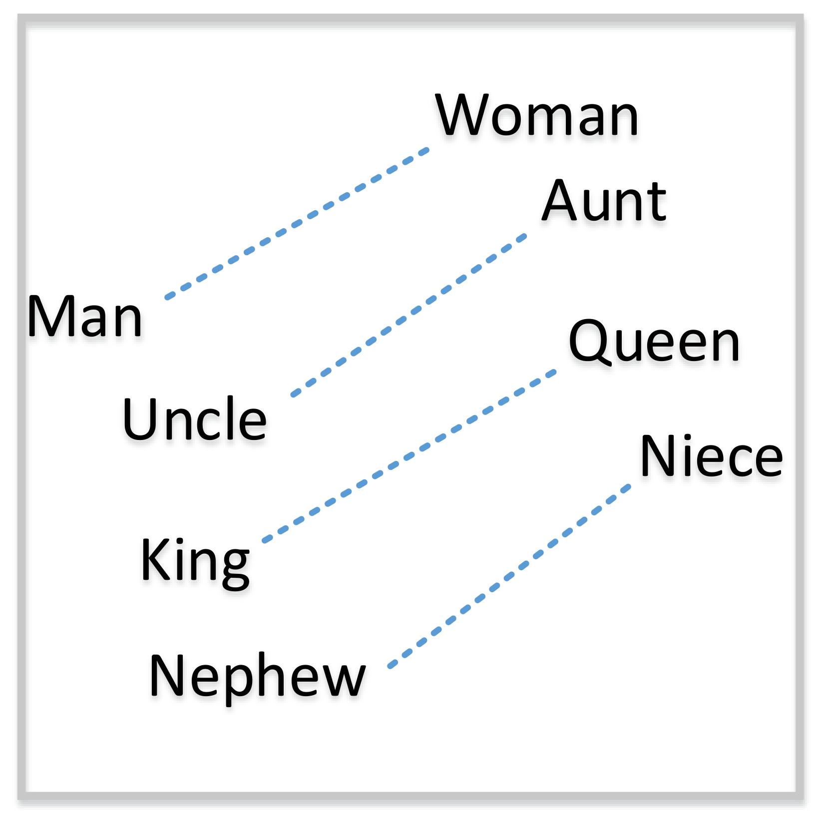
2.4. Word Embedding
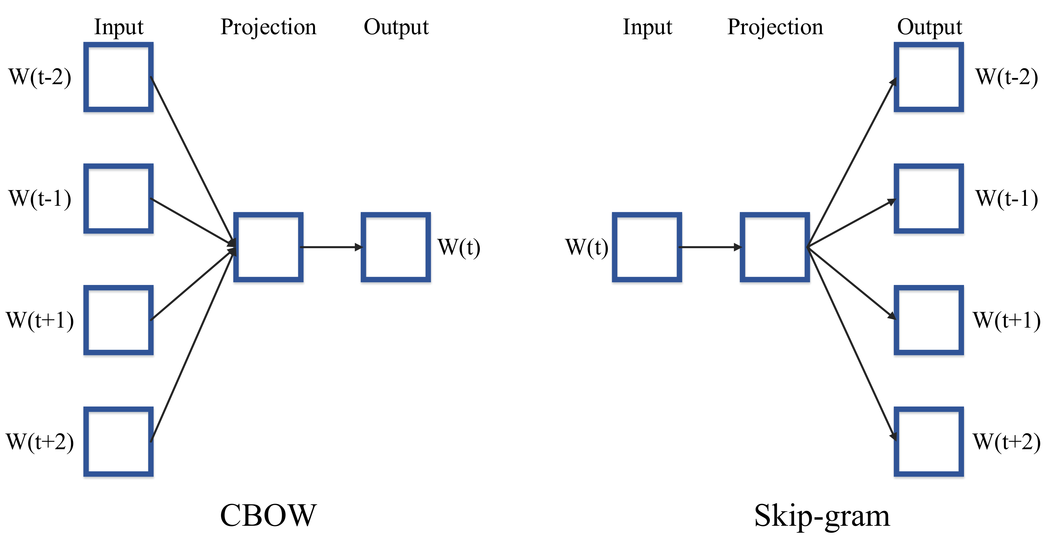
2.4.1. Word2Vec
Continuous Bag-of-Words Model
Continuous Skip-Gram Model
2.4.2. Global Vectors for Word Representation (GloVe)
2.4.3. FastText
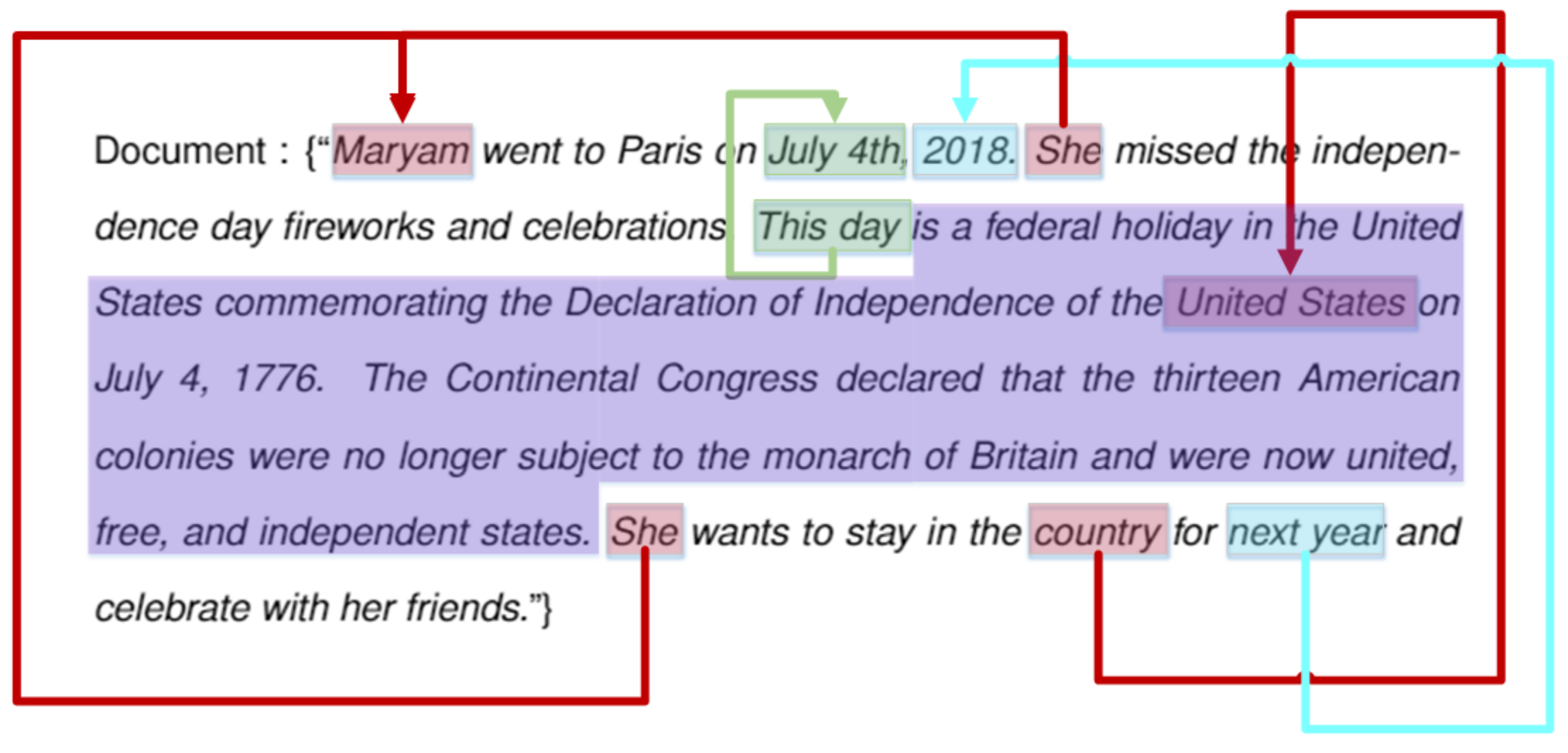
2.4.4. Contextualized Word Representations
2.5. Limitations
3. Dimensionality Reduction
3.1. Component Analysis
3.1.1. Principal Component Analysis (PCA)
3.1.2. Independent Component Analysis (ICA)
3.2. Linear Discriminant Analysis (LDA)
3.3. Non-Negative Matrix Factorization (NMF)
- (I)
- Extract index term after pre-processing stem like feature extraction and text cleaning as discussed in Section 2. Then we have n documents with m features;
- (II)
- Create n documents (), where vector where refers to local weights of term in document j, and is global weights for document i;
- (III)
- Apply NMF to all terms in all documents one by one;
- (IV)
- Project the trained document vector into r-dimensional space;
- (V)
- Using the same transformation, map the test set into the r-dimensional space;
- (VI)
- Calculate the similarity between the transformed document vectors and a query vector.
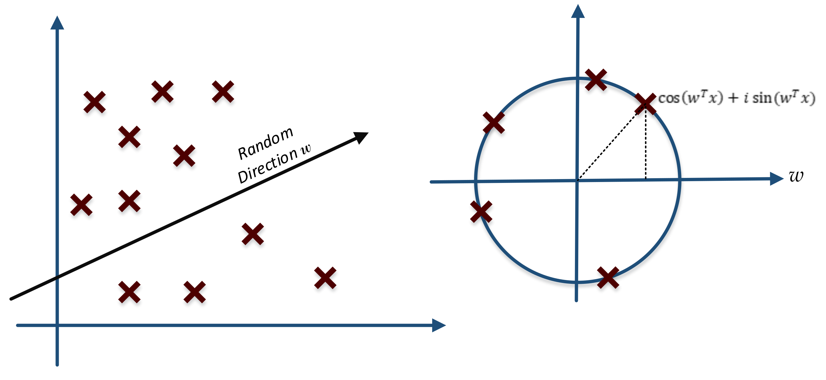
3.4. Random Projection
3.4.1. Random Kitchen Sinks
3.4.2. Johnson Lindenstrauss Lemma
Johnson Lindenstrauss Lemma Proof [89]:
Lemma 1 Proof [89]:
Lemma 2 Proof [89]:
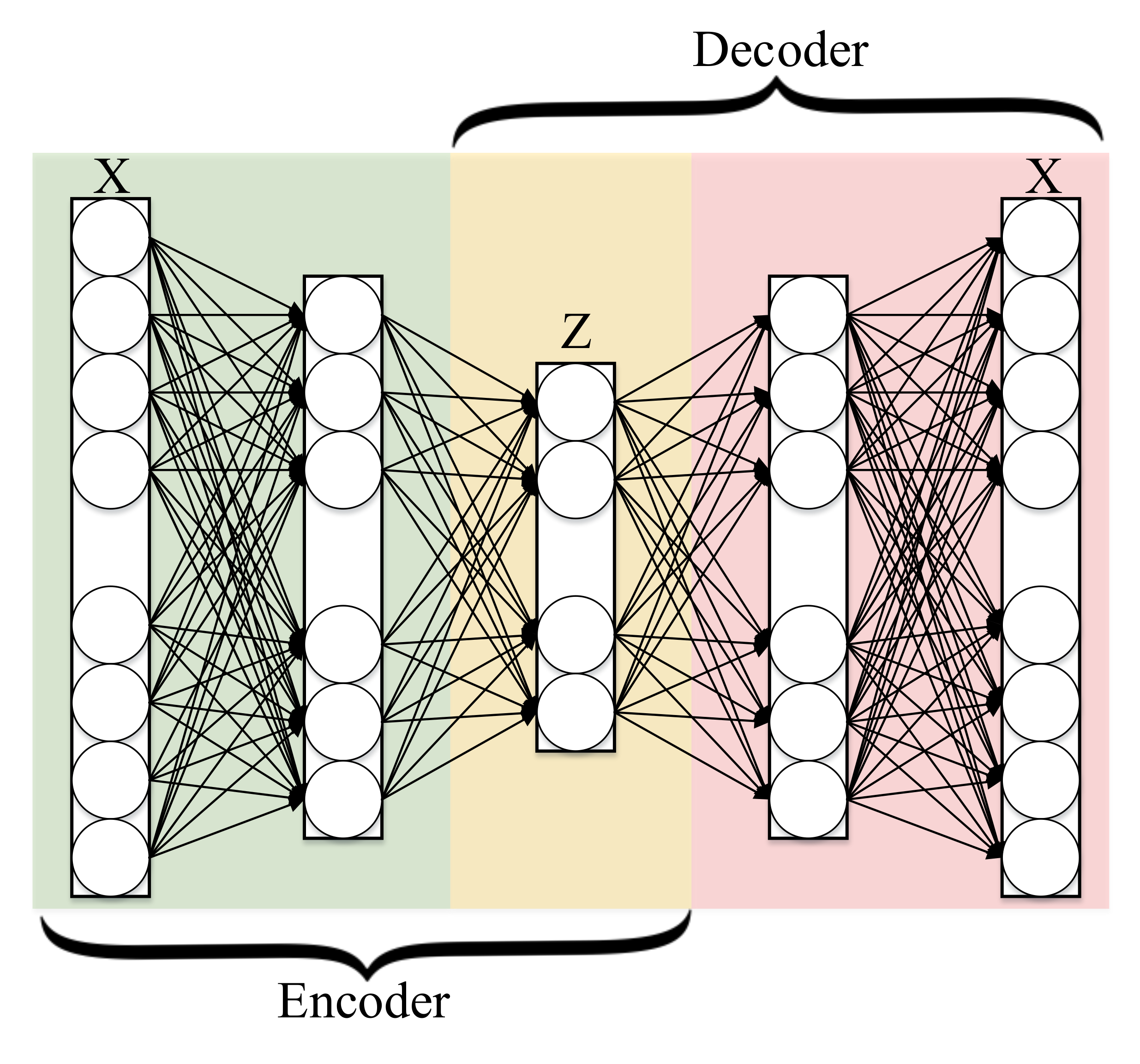
3.5. Autoencoder
3.5.1. General Framework
3.5.2. Conventional Autoencoder Architecture
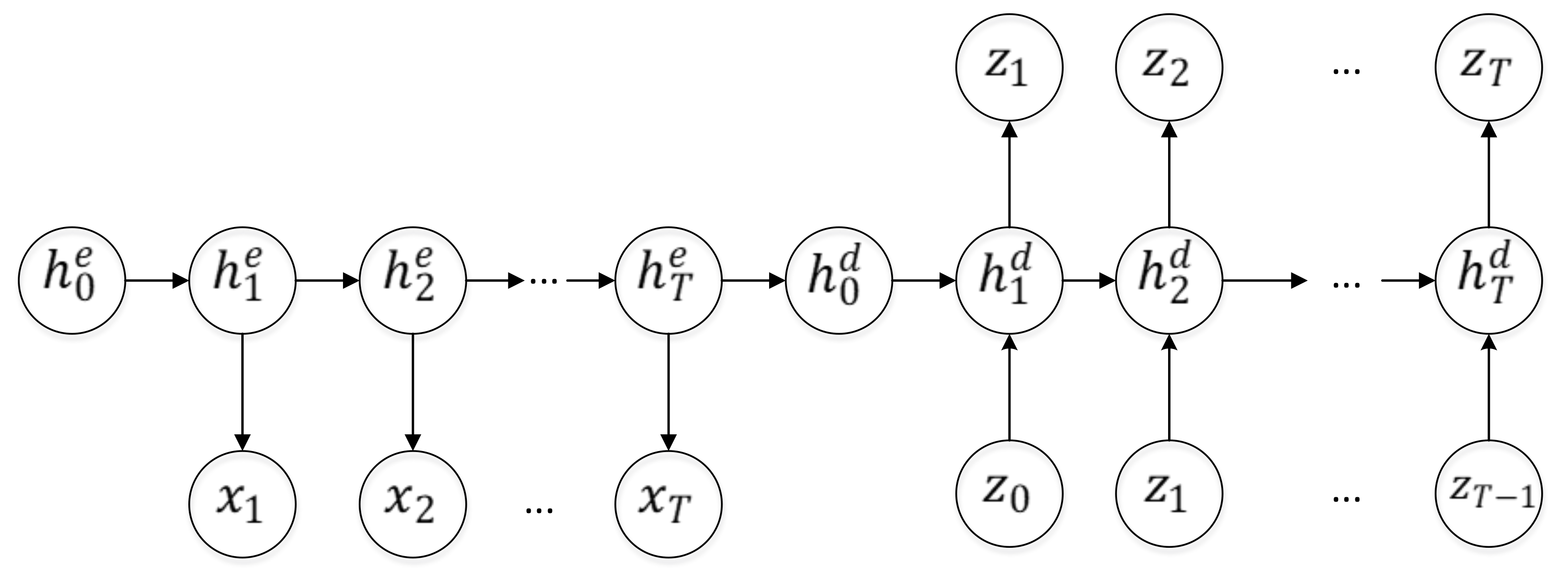
3.5.3. Recurrent Autoencoder Architecture
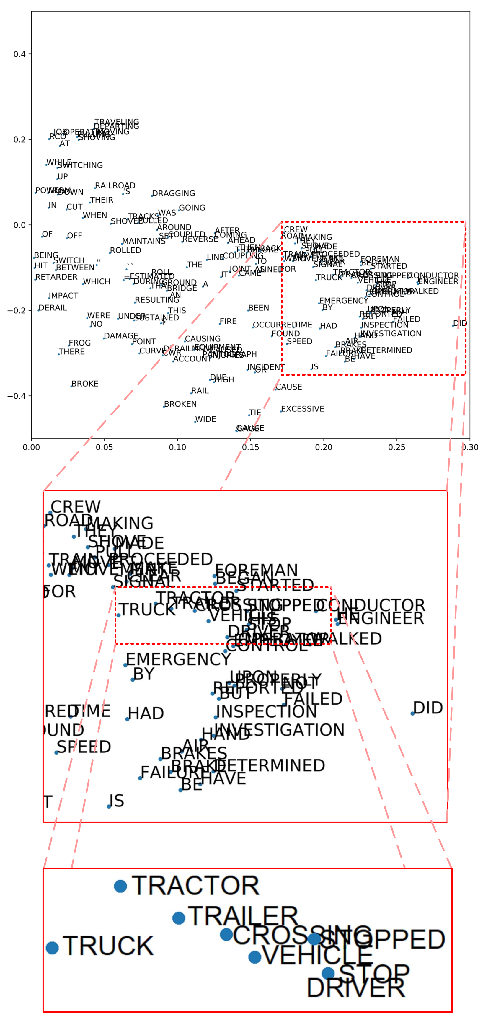
3.6. T-Distributed Stochastic Neighbor Embedding (t-SNE)
4. Existing Classification Techniques
4.1. Rocchio Classification
Limitation of Rocchio Algorithm
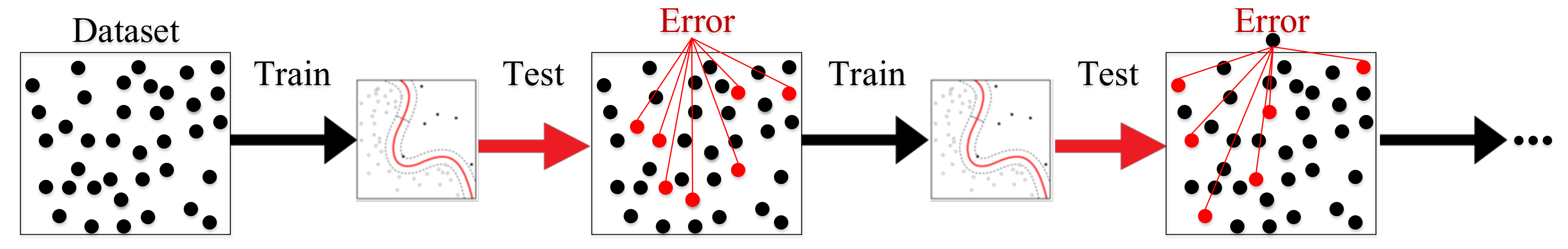
4.2. Boosting and Bagging
4.2.1. Boosting
| Algorithm 1 The AdaBoost method |
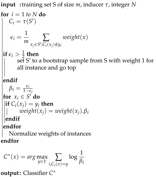 |
4.2.2. Bagging
| Algorithm 2 Bagging |
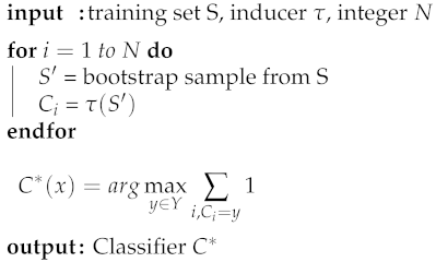 |
4.2.3. Limitation of Boosting and Bagging
4.3. Logistic Regression
4.3.1. Basic Framework
4.3.2. Combining Instance-Based Learning and LR
4.3.3. Multinomial Logistic Regression
4.3.4. Limitation of Logistic Regression
4.4. Naïve Bayes Classifier
4.4.1. High-Level Description of Naïve Bayes Classifier
4.4.2. Multinomial Naïve Bayes Classifier
4.4.3. Naïve Bayes Classifier for Unbalanced Classes
4.4.4. Limitation of Naïve Bayes Algorithm
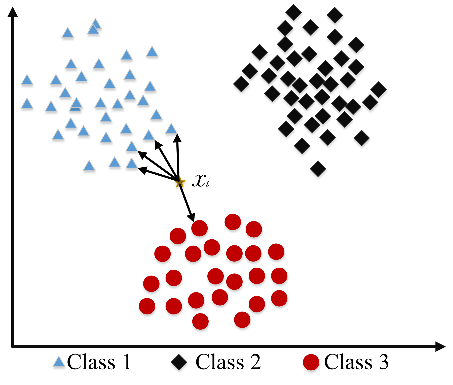
4.5. K-Nearest Neighbor
4.5.1. Basic Concept of KNN
4.5.2. Weight Adjusted K-Nearest Neighbor Classification
4.5.3. Limitation of K-Nearest Neighbor
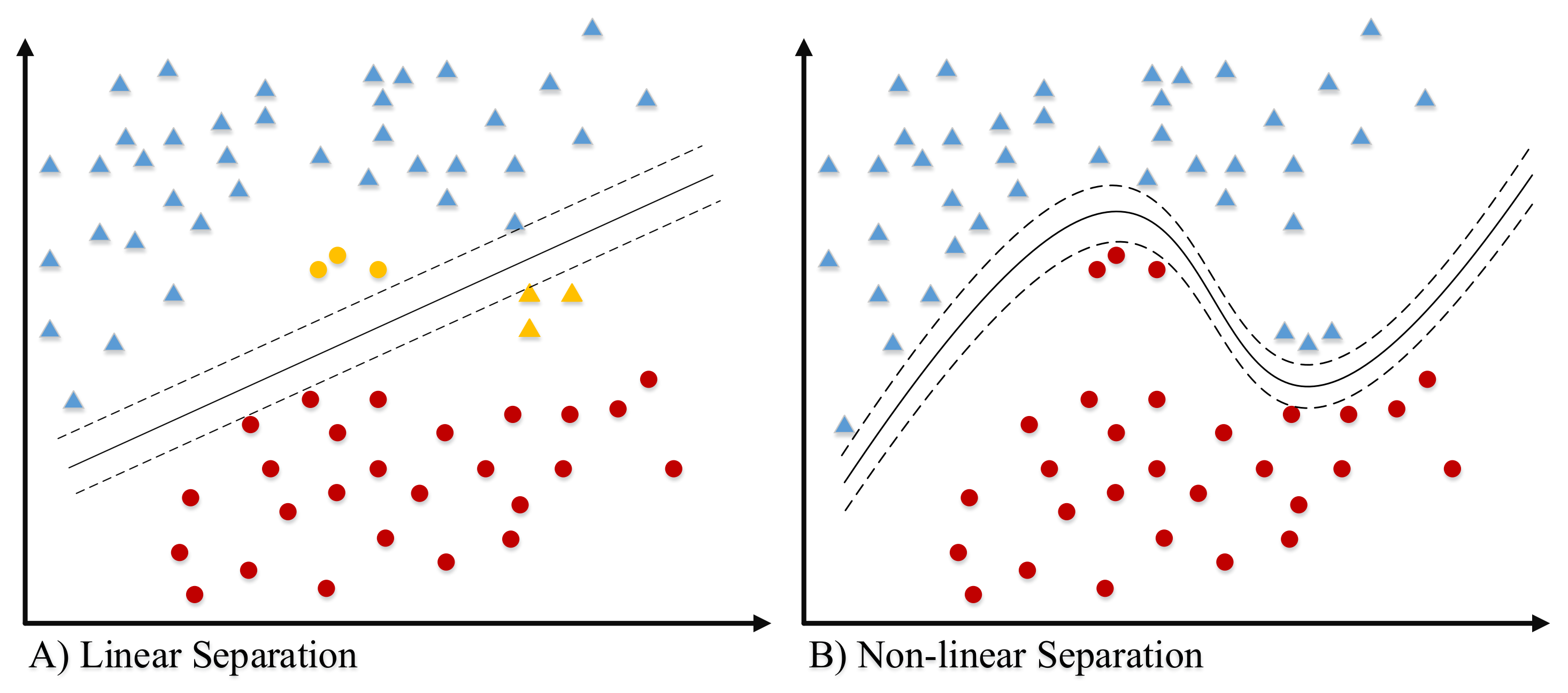
4.6. Support Vector Machine (SVM)
4.6.1. Binary-Class SVM
4.6.2. Multi-Class SVM
4.6.3. String Kernel
4.6.4. Stacking Support Vector Machine (SVM)
4.6.5. Multiple Instance Learning (MIL)
4.6.6. Limitation of Support Vector Machine (SVM)
4.7. Decision Tree
Limitation of Decision Tree Algorithm
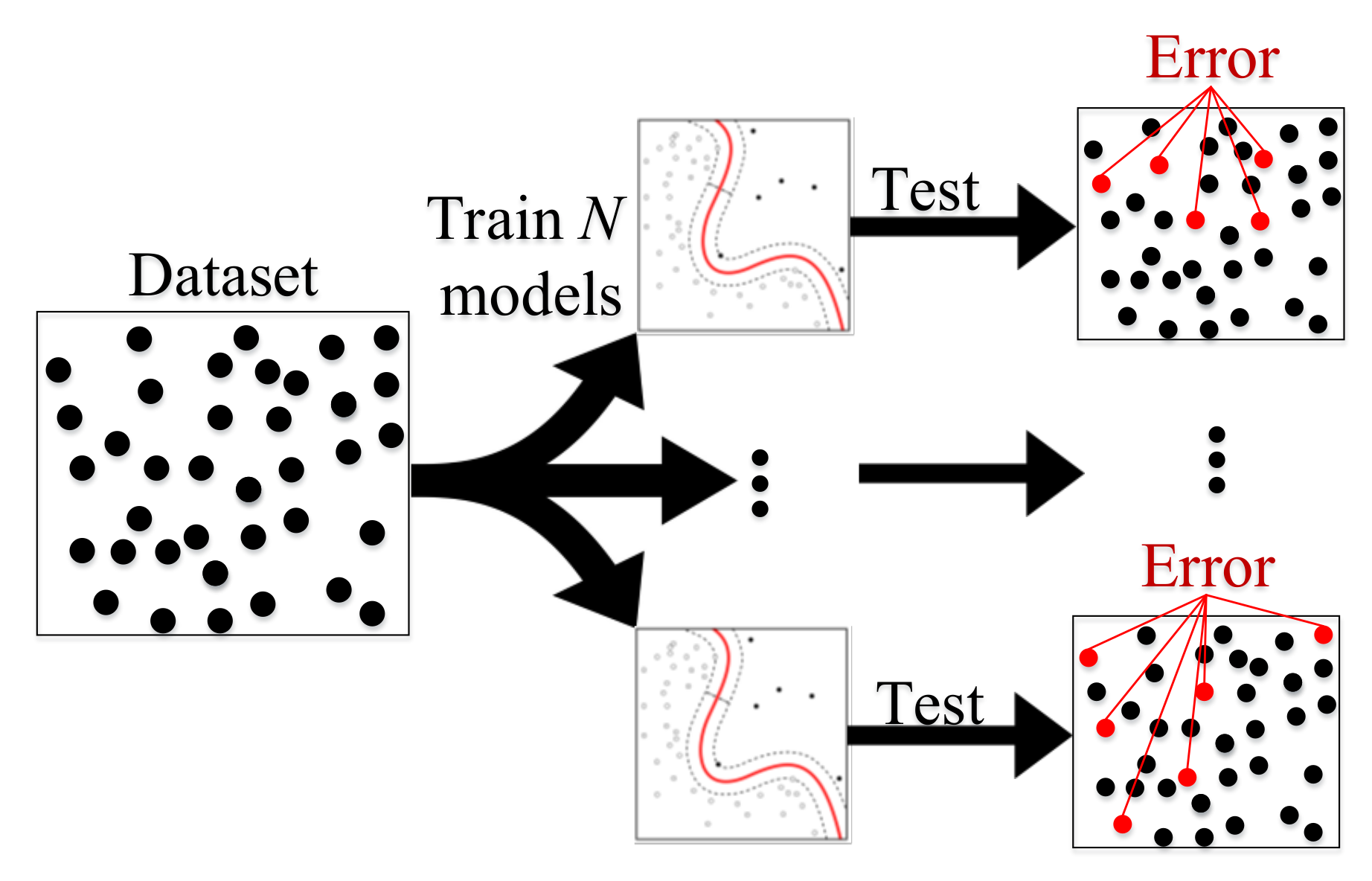
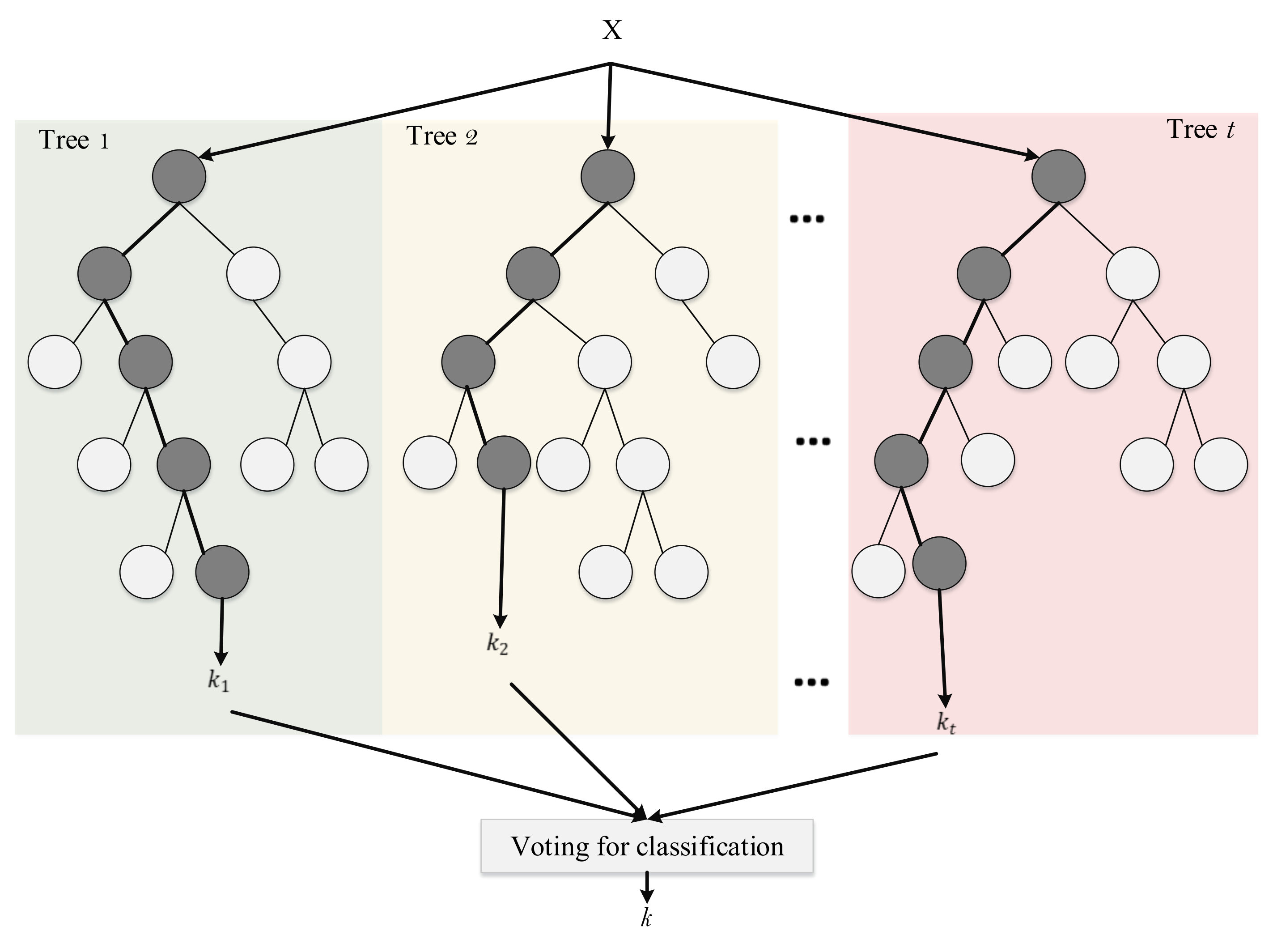
4.8. Random Forest
4.8.1. Voting
4.8.2. Limitation of Random Forests
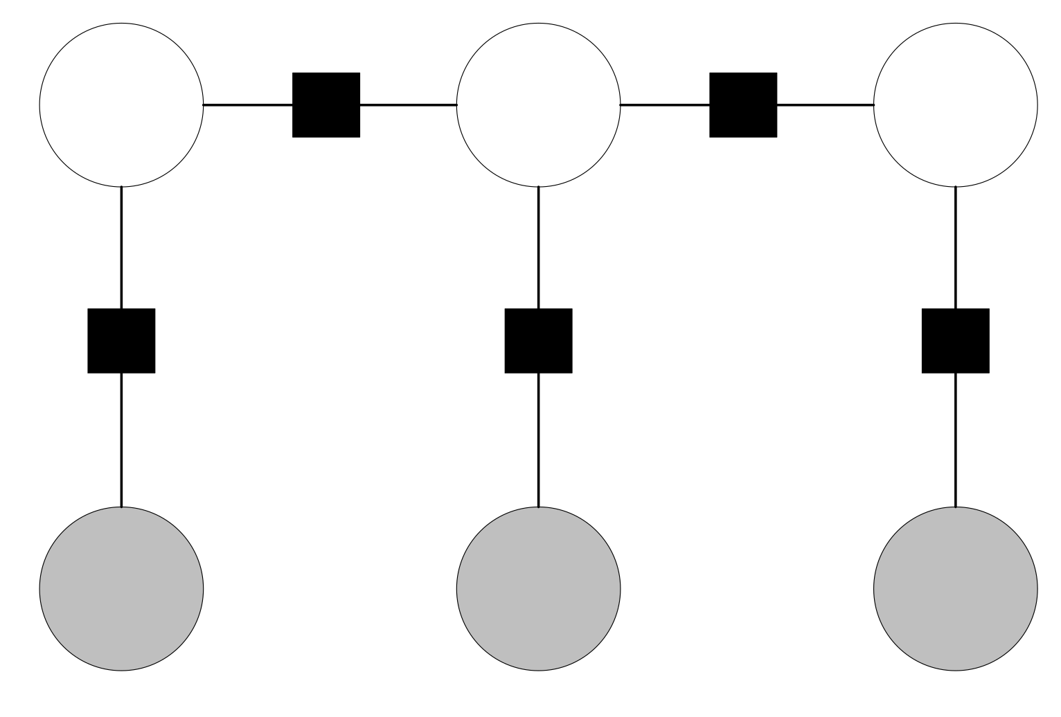
4.9. Conditional Random Field (CRF)
Limitation of Conditional Random Field (CRF)
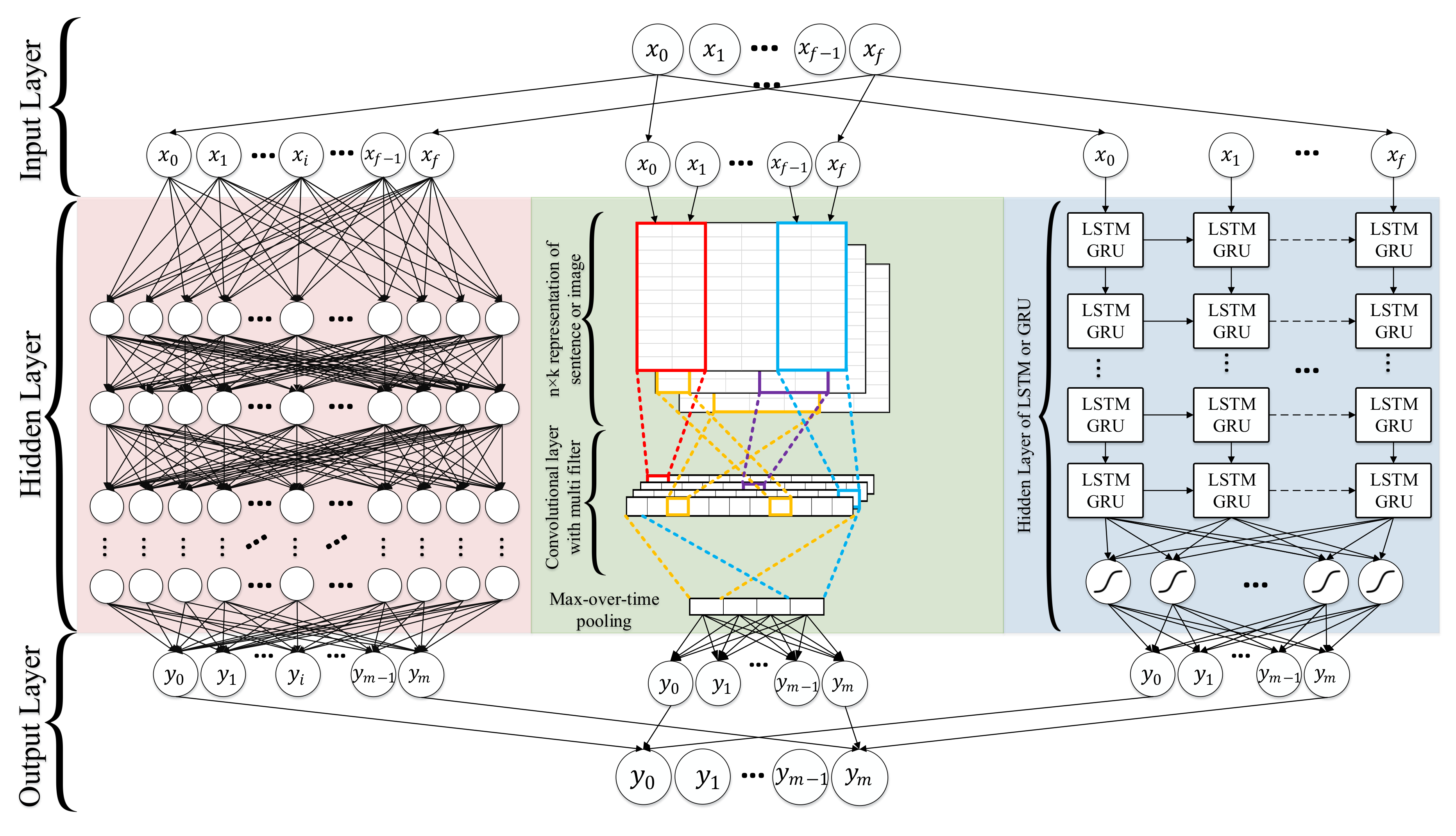
4.10. Deep Learning
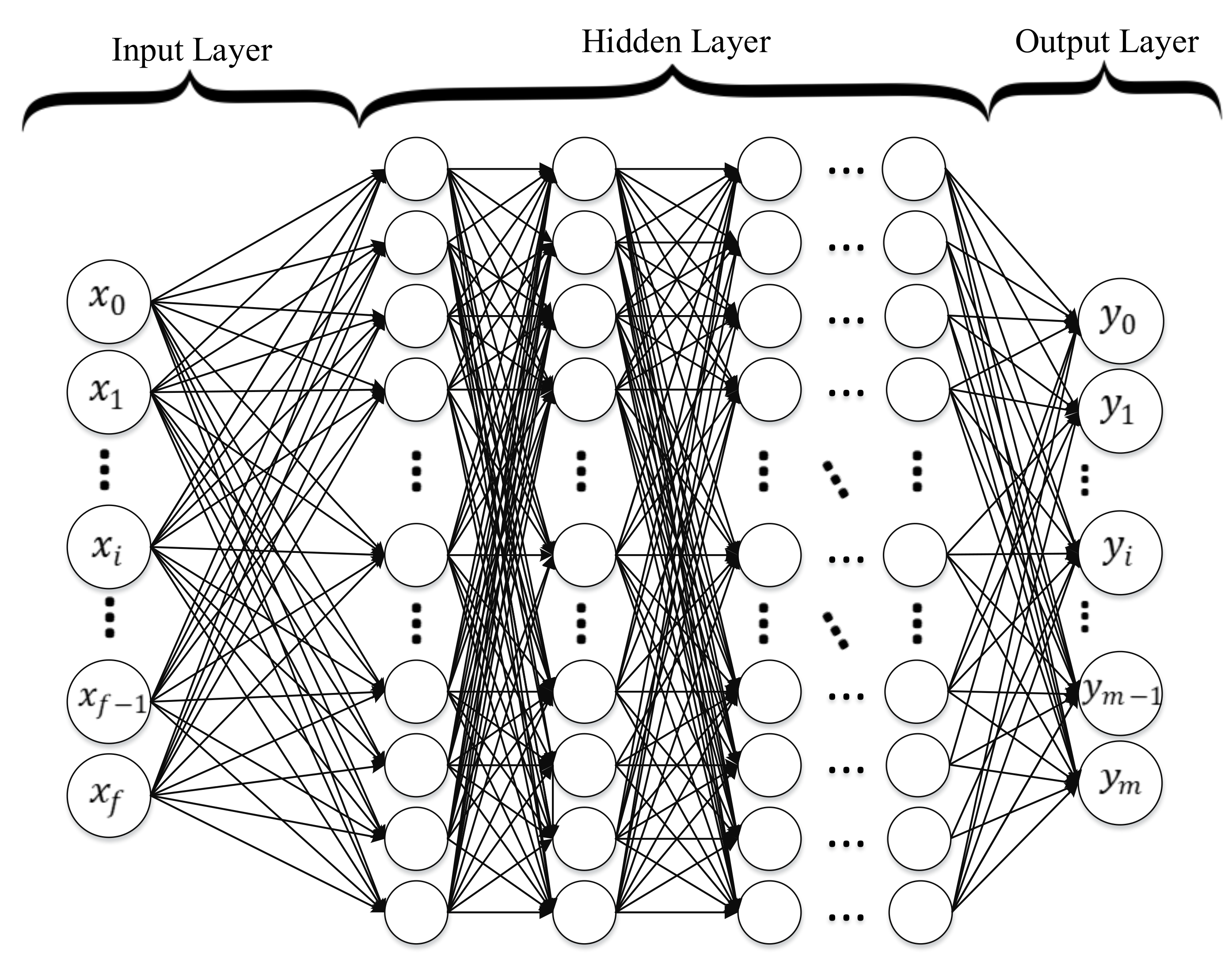
4.10.1. Deep Neural Networks
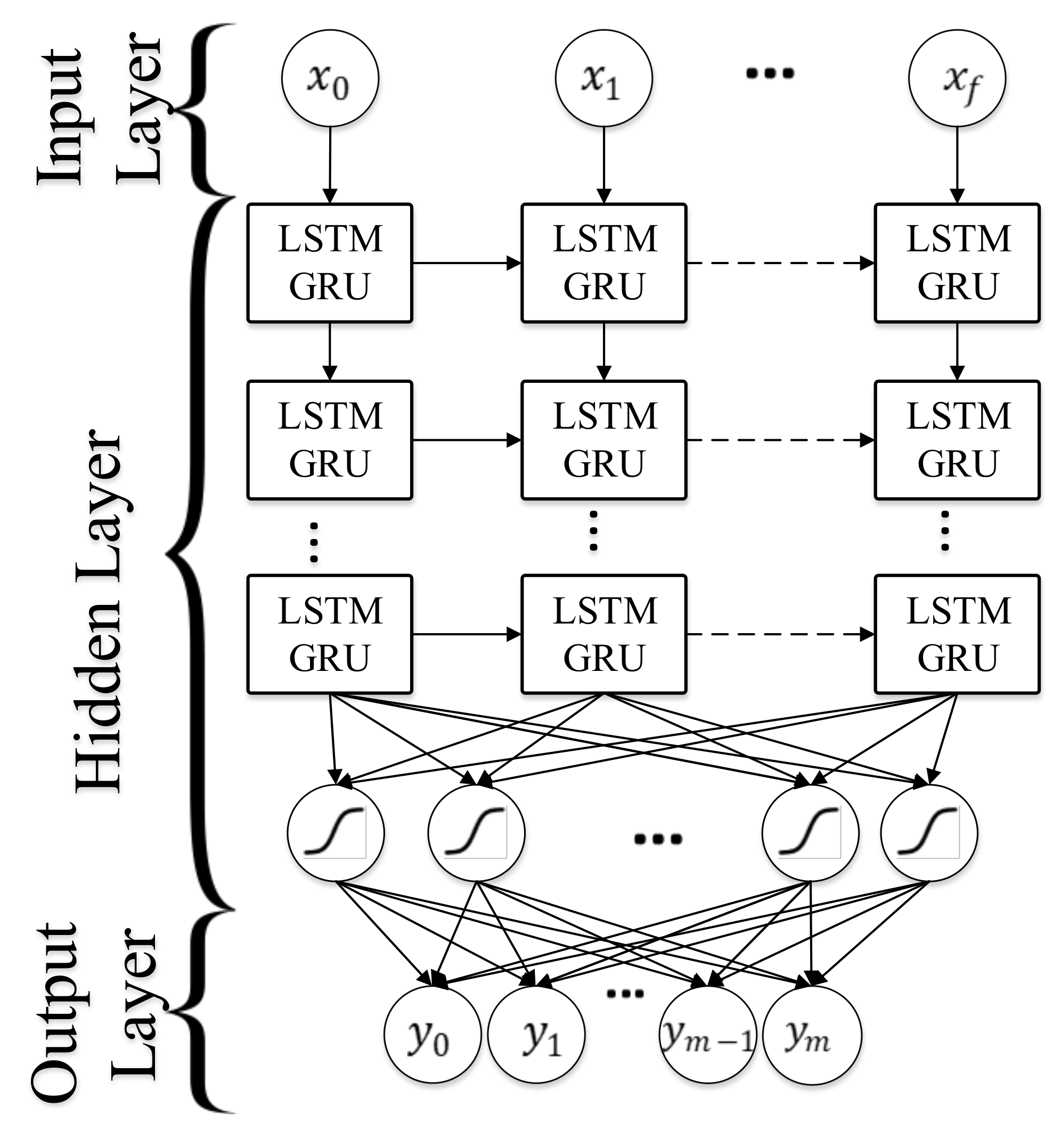
4.10.2. Recurrent Neural Network (RNN)
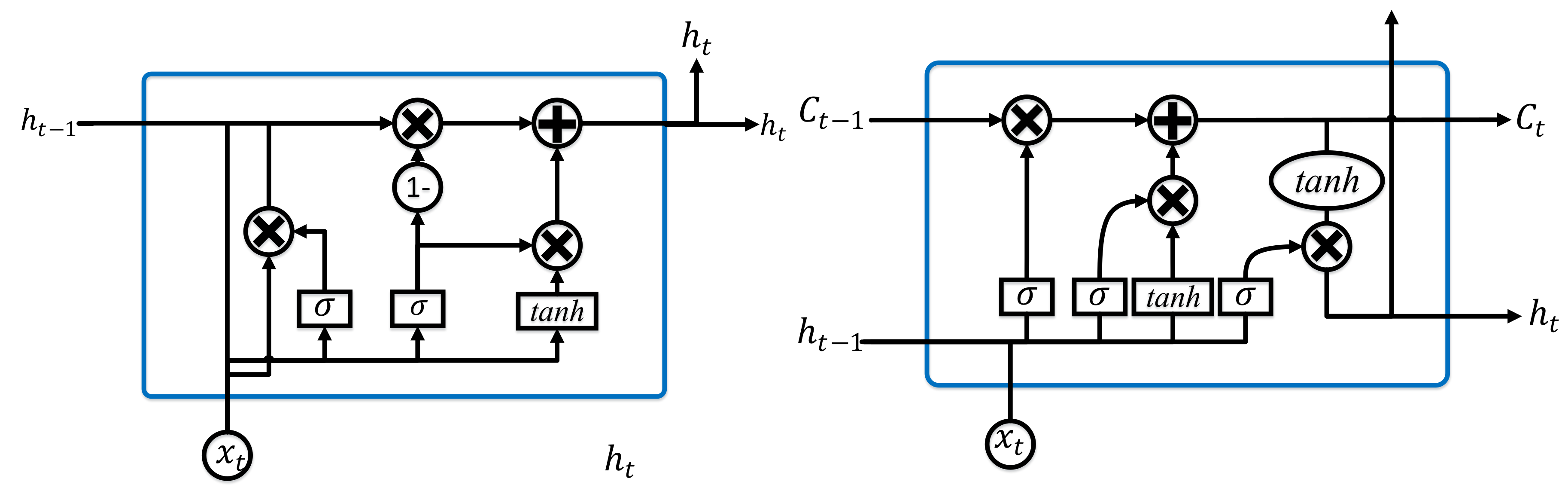
Long Short-Term Memory (LSTM)
Gated Recurrent Unit (GRU)
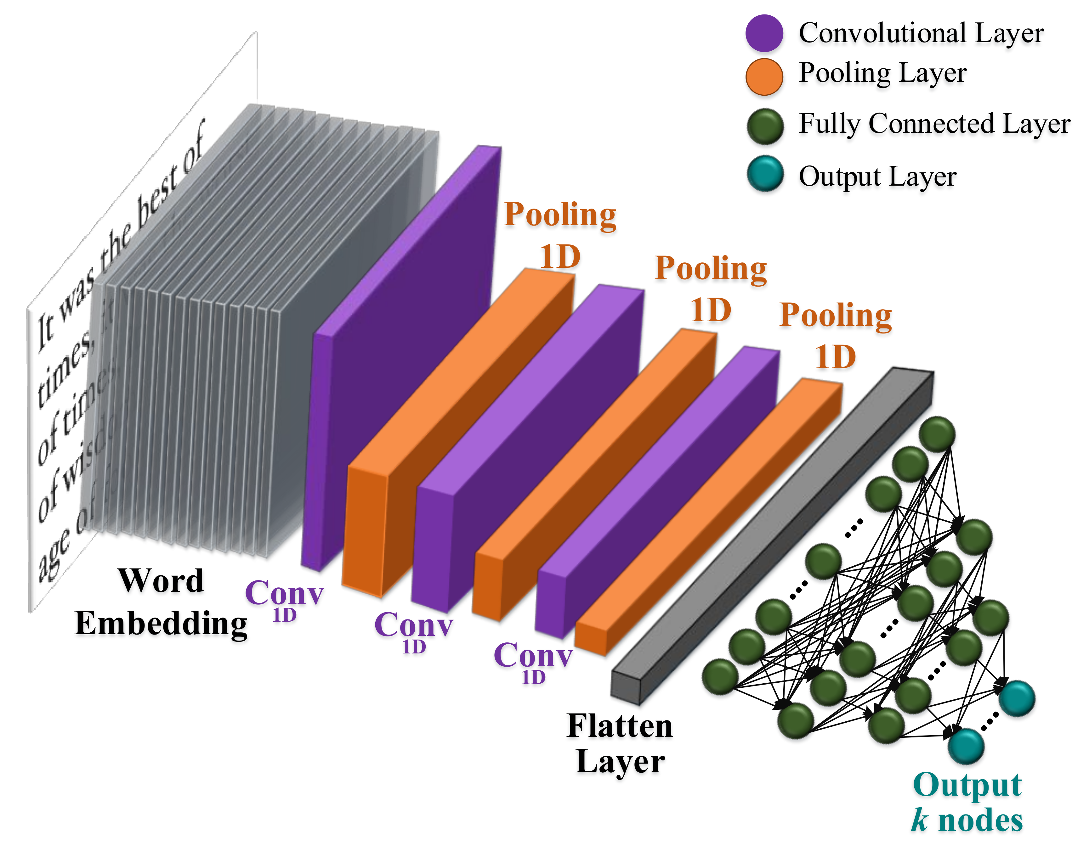
4.10.3. Convolutional Neural Networks (CNN)
4.10.4. Deep Belief Network (DBN)
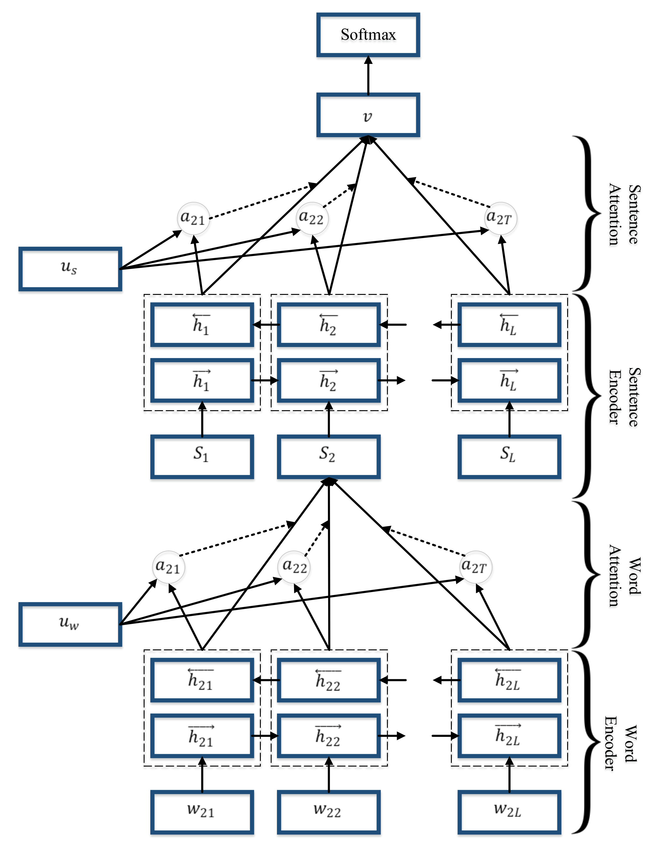
4.10.5. Hierarchical Attention Networks (HAN)
4.10.6. Combination Techniques
Random Multimodel Deep Learning (RMDL)
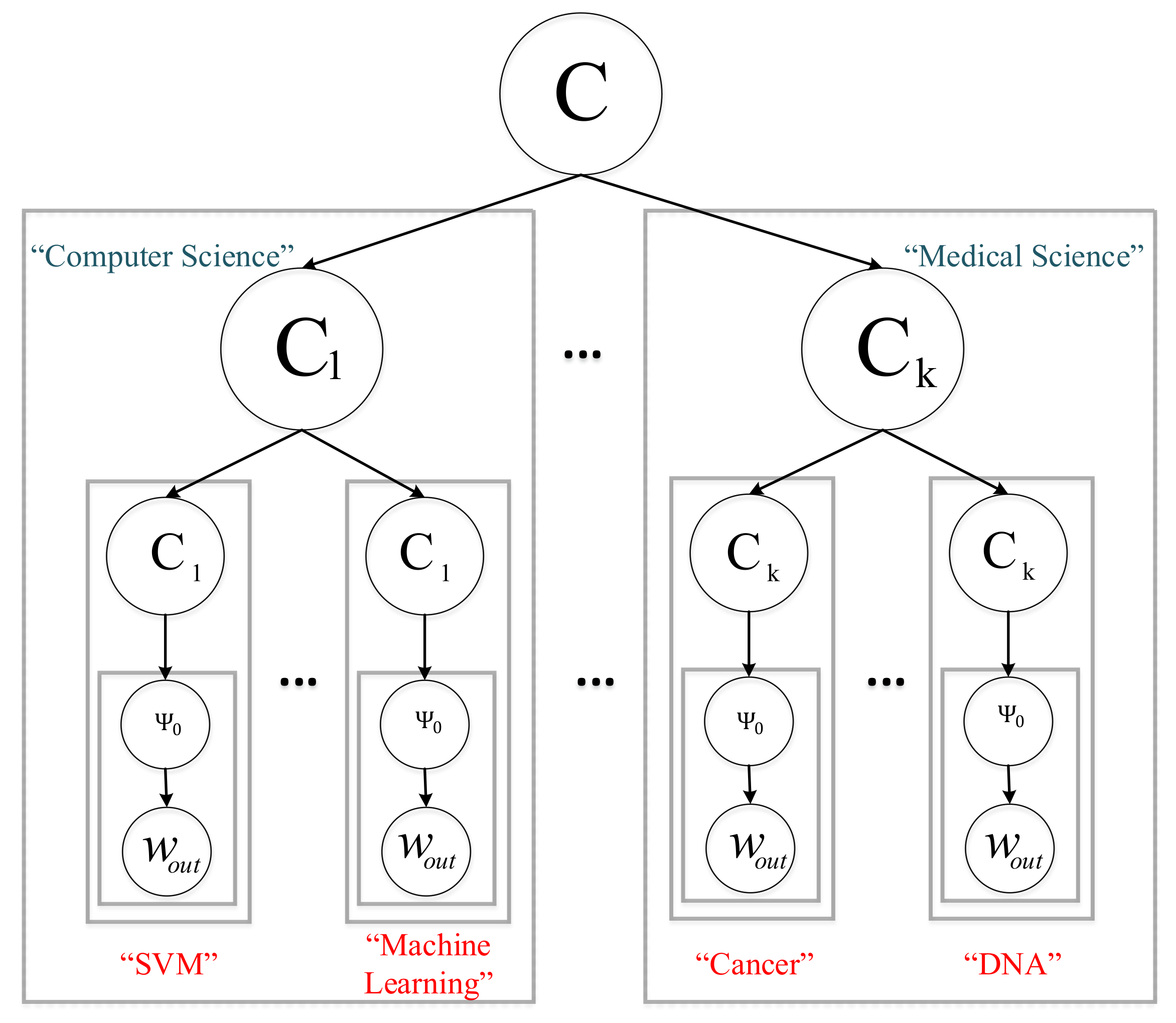
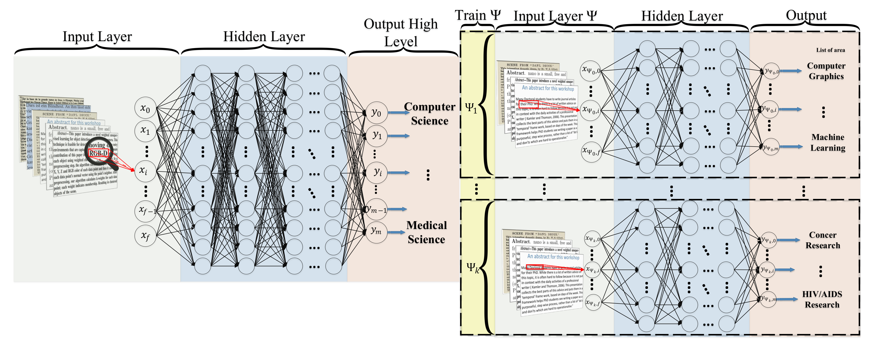
Hierarchical Deep Learning for Text (HDLTex)
- DNN:
- 8 hidden layers with 1024 cells in each hidden layer.
- RNN:
- GRU and LSTM are used in this implementation, 100 cells with GRU with two hidden layers.
- CNN:
- Filter sizes of and max-pool of 5, layer sizes of with max pooling of , the CNN contains 8 hidden layers.
Other Techniques
4.10.7. Limitation of Deep Learning
4.11. Semi-Supervised Learning for Text Classification
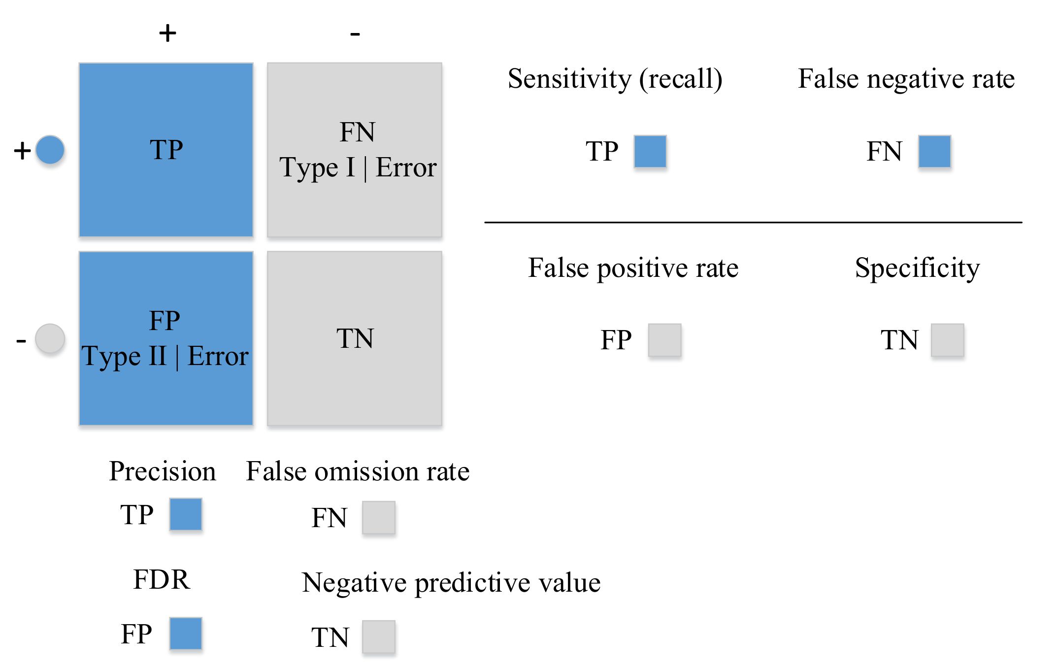
5. Evaluation
5.1. Macro-Averaging and Micro-Averaging
5.2. F Score
5.3. Matthews Correlation Coefficient (MCC)
5.4. Receiver Operating Characteristics (ROC)
5.5. Area Under ROC Curve (AUC)
- Comparative evaluation across methods and experiments which gives insight about factors underlying performance variations and will lead to better evaluation methodology in the future;
- Impact of collection variability such as including unlabeled documents in training or test set and treat them as negative instances can be a serious problem;
- Category ranking evaluation and binary classification evaluation show the usefulness of classifier in interactive applications and emphasize their use in a batch mode respectively. Having both types of performance measurements to rank classifiers is helpful in detecting the effects of thresholding strategies;
- Evaluation of the scalability of classifiers in large category spaces is a rarely investigated area.
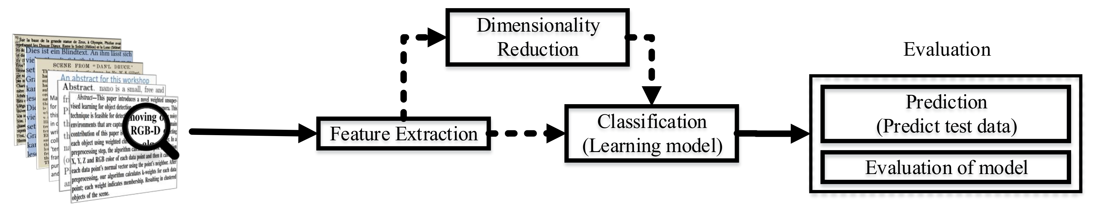
6. Discussion
6.1. Text and Document Feature Extraction
6.2. Dimensionality Reduction
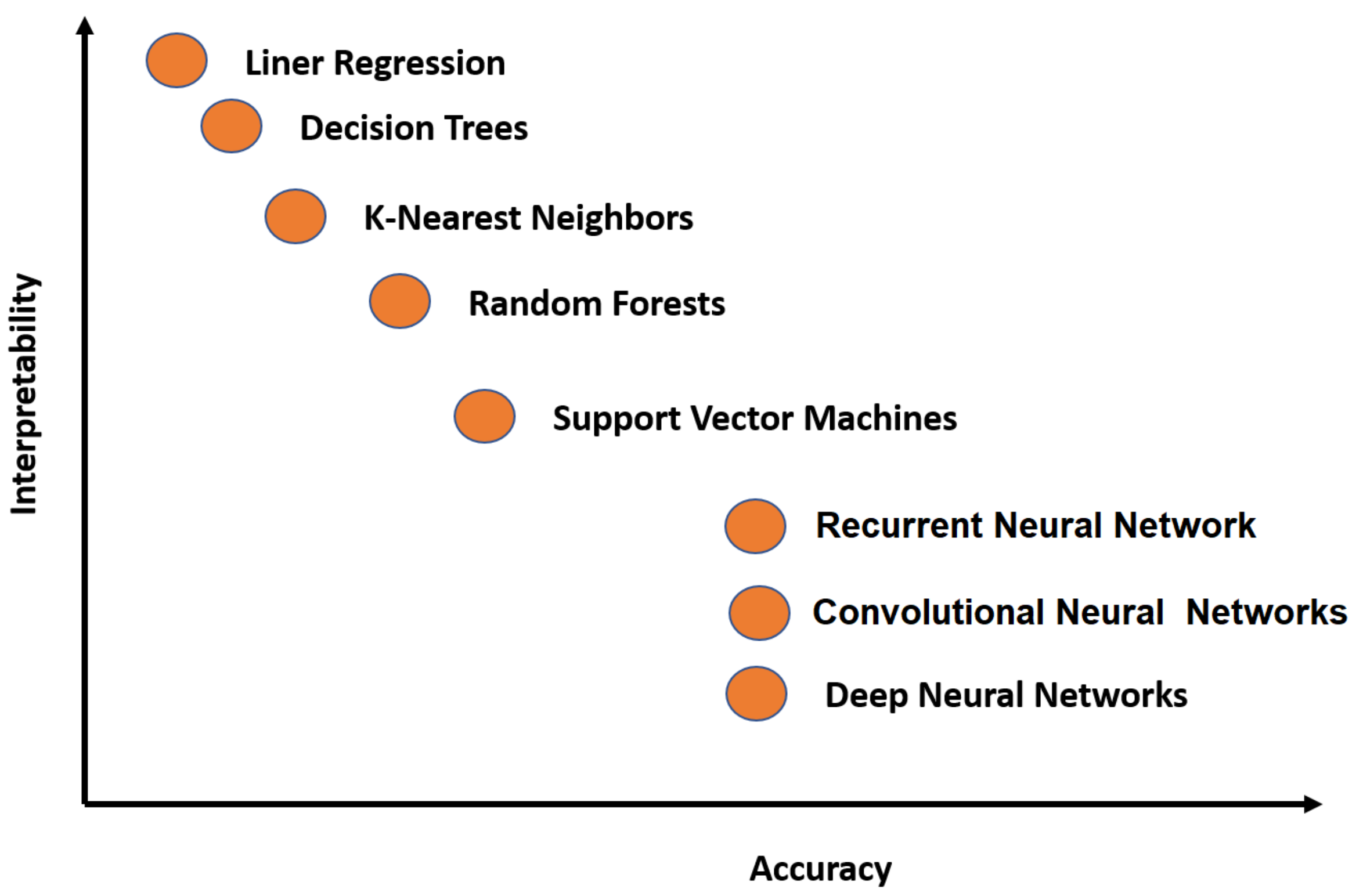
6.3. Existing Classification Techniques
6.3.1. Limitations and Advantages
6.3.2. State-of-the-Art Techniques’ Comparison
6.4. Evaluation
7. Text Classification Usage
7.1. Text Classification Applications
7.1.1. Information Retrieval
7.1.2. Information Filtering
7.1.3. Sentiment Analysis
7.1.4. Recommender Systems
7.1.5. Knowledge Management
7.1.6. Document Summarization
7.2. Text Classification Support
7.2.1. Health
7.2.2. Social Sciences
7.2.3. Business and Marketing
7.2.4. Law
8. Conclusions
Author Contributions
Funding
Acknowledgments
Conflicts of Interest
References
- Jiang, M.; Liang, Y.; Feng, X.; Fan, X.; Pei, Z.; Xue, Y.; Guan, R. Text classification based on deep belief network and softmax regression. Neural Comput. Appl. 2018, 29, 61–70. [Google Scholar] [CrossRef]
- Kowsari, K.; Brown, D.E.; Heidarysafa, M.; Jafari Meimandi, K.; Gerber, M.S.; Barnes, L.E. HDLTex: Hierarchical Deep Learning for Text Classification. Machine Learning and Applications (ICMLA). In Proceedings of the 2017 16th IEEE International Conference on Machine Learning and Applications (ICMLA), Cancun, Mexico, 18–21 December 2017. [Google Scholar]
- McCallum, A.; Nigam, K. A comparison of event models for naive bayes text classification. In Proceedings of the AAAI-98 Workshop on Learning for Text Categorization, Madison, WI, USA, 26–27 July 1998; Volume 752, pp. 41–48. [Google Scholar]
- Kowsari, K.; Heidarysafa, M.; Brown, D.E.; Jafari Meimandi, K.; Barnes, L.E. RMDL: Random Multimodel Deep Learning for Classification. In Proceedings of the 2018 International Conference on Information System and Data Mining, Lakeland, FL, USA, 9–11 April 2018. [Google Scholar] [CrossRef]
- Heidarysafa, M.; Kowsari, K.; Brown, D.E.; Jafari Meimandi, K.; Barnes, L.E. An Improvement of Data Classification Using Random Multimodel Deep Learning (RMDL). IJMLC 2018, 8, 298–310. [Google Scholar] [CrossRef]
- Lai, S.; Xu, L.; Liu, K.; Zhao, J. Recurrent Convolutional Neural Networks for Text Classification. In Proceedings of the Twenty-Ninth AAAI Conference on Artificial Intelligence, Austin, TX, USA, 25–30 January 2015; Volume 333, pp. 2267–2273. [Google Scholar]
- Aggarwal, C.C.; Zhai, C. A survey of text classification algorithms. In Mining Text Data; Springer: Berlin/Heidelberg, Germany, 2012; pp. 163–222. [Google Scholar]
- Aggarwal, C.C.; Zhai, C.X. Mining Text Data; Springer: Berlin/Heidelberg, Germany, 2012. [Google Scholar]
- Salton, G.; Buckley, C. Term-weighting approaches in automatic text retrieval. Inf. Process. Manag. 1988, 24, 513–523. [Google Scholar] [CrossRef]
- Goldberg, Y.; Levy, O. Word2vec explained: Deriving mikolov et al.’s negative-sampling word-embedding method. arXiv 2014, arXiv:1402.3722. [Google Scholar]
- Pennington, J.; Socher, R.; Manning, C.D. Glove: Global Vectors for Word Representation. In Proceedings of the 2014 Conference on Empirical Methods in Natural Language Processing (EMNLP), Doha, Qatar, 25–29 October 2014; Volume 14, pp. 1532–1543. [Google Scholar]
- Mamitsuka, N.A.H. Query learning strategies using boosting and bagging. In Machine Learning: Proceedings of the Fifteenth International Conference (ICML’98); Morgan Kaufmann Pub.: Burlington, MA, USA, 1998; Volume 1. [Google Scholar]
- Kim, Y.H.; Hahn, S.Y.; Zhang, B.T. Text filtering by boosting naive Bayes classifiers. In Proceedings of the 23rd Annual International ACM SIGIR Conference on Research and Development in Information Retrieval, Athens, Greece, 24–28 July 2000; pp. 168–175. [Google Scholar]
- Schapire, R.E.; Singer, Y. BoosTexter: A boosting-based system for text categorization. Mach. Learn. 2000, 39, 135–168. [Google Scholar] [CrossRef]
- Harrell, F.E. Ordinal logistic regression. In Regression Modeling Strategies; Springer: Berlin/Heidelberg, Germany, 2001; pp. 331–343. [Google Scholar]
- Hosmer, D.W., Jr.; Lemeshow, S.; Sturdivant, R.X. Applied Logistic Regression; John Wiley & Sons: Hoboken, NJ, USA, 2013; Volume 398. [Google Scholar]
- Dou, J.; Yamagishi, H.; Zhu, Z.; Yunus, A.P.; Chen, C.W. TXT-tool 1.081-6.1 A Comparative Study of the Binary Logistic Regression (BLR) and Artificial Neural Network (ANN) Models for GIS-Based Spatial Predicting Landslides at a Regional Scale. In Landslide Dynamics: ISDR-ICL Landslide Interactive Teaching Tools; Springer: Berlin/Heidelberg, Germany, 2018; pp. 139–151. [Google Scholar]
- Chen, W.; Xie, X.; Wang, J.; Pradhan, B.; Hong, H.; Bui, D.T.; Duan, Z.; Ma, J. A comparative study of logistic model tree, random forest, and classification and regression tree models for spatial prediction of landslide susceptibility. Catena 2017, 151, 147–160. [Google Scholar] [CrossRef]
- Larson, R.R. Introduction to information retrieval. J. Am. Soc. Inf. Sci. Technol. 2010, 61, 852–853. [Google Scholar] [CrossRef]
- Li, L.; Weinberg, C.R.; Darden, T.A.; Pedersen, L.G. Gene selection for sample classification based on gene expression data: Study of sensitivity to choice of parameters of the GA/KNN method. Bioinformatics 2001, 17, 1131–1142. [Google Scholar] [CrossRef]
- Manevitz, L.M.; Yousef, M. One-class SVMs for document classification. J. Mach. Learn. Res. 2001, 2, 139–154. [Google Scholar]
- Han, E.H.S.; Karypis, G. Centroid-based document classification: Analysis and experimental results. In European Conference on Principles of Data Mining and Knowledge Discovery; Springer: Berlin/Heidelberg, Germany, 2000; pp. 424–431. [Google Scholar]
- Xu, B.; Guo, X.; Ye, Y.; Cheng, J. An Improved Random Forest Classifier for Text Categorization. JCP 2012, 7, 2913–2920. [Google Scholar] [CrossRef]
- Lafferty, J.; McCallum, A.; Pereira, F.C. Conditional random fields: Probabilistic models for segmenting and labeling sequence data. In Proceedings of the 18th International Conference on Machine Learning 2001 (ICML 2001), Williamstown, MA, USA, 28 June–1 July 2001. [Google Scholar]
- Shen, D.; Sun, J.T.; Li, H.; Yang, Q.; Chen, Z. Document Summarization Using Conditional Random Fields. IJCAI 2007, 7, 2862–2867. [Google Scholar]
- Zhang, C. Automatic keyword extraction from documents using conditional random fields. J. Comput. Inf. Syst. 2008, 4, 1169–1180. [Google Scholar]
- LeCun, Y.; Bengio, Y.; Hinton, G. Deep learning. Nature 2015, 521, 436–444. [Google Scholar] [CrossRef] [PubMed]
- Huang, J.; Ling, C.X. Using AUC and accuracy in evaluating learning algorithms. IEEE Trans. Knowl. Data Eng. 2005, 17, 299–310. [Google Scholar] [CrossRef]
- Lock, G. Acute mesenteric ischemia: Classification, evaluation and therapy. Acta Gastro-Enterol. Belg. 2002, 65, 220–225. [Google Scholar]
- Matthews, B.W. Comparison of the predicted and observed secondary structure of T4 phage lysozyme. Biochim. Biophys. Acta (BBA)-Protein Struct. 1975, 405, 442–451. [Google Scholar] [CrossRef]
- Hanley, J.A.; McNeil, B.J. The meaning and use of the area under a receiver operating characteristic (ROC) curve. Radiology 1982, 143, 29–36. [Google Scholar] [CrossRef]
- Pencina, M.J.; D’Agostino, R.B.; Vasan, R.S. Evaluating the added predictive ability of a new marker: From area under the ROC curve to reclassification and beyond. Stat. Med. 2008, 27, 157–172. [Google Scholar] [CrossRef]
- Jacobs, P.S. Text-Based Intelligent Systems: Current Research and Practice in Information Extraction and Retrieval; Psychology Press: Hove, UK, 2014. [Google Scholar]
- Croft, W.B.; Metzler, D.; Strohman, T. Search Engines: Information Retrieval in Practice; Addison-Wesley Reading: Boston, MA, USA, 2010; Volume 283. [Google Scholar]
- Yammahi, M.; Kowsari, K.; Shen, C.; Berkovich, S. An efficient technique for searching very large files with fuzzy criteria using the pigeonhole principle. In Proceedings of the 2014 Fifth International Conference on Computing for Geospatial Research and Application, Washington, DC, USA, 4–6 August 2014; pp. 82–86. [Google Scholar]
- Chu, Z.; Gianvecchio, S.; Wang, H.; Jajodia, S. Who is tweeting on Twitter: Human, bot, or cyborg? In Proceedings of the 26th Annual Computer Security Applications Conference, Austin, TX, USA, 6–10 December 2010; pp. 21–30. [Google Scholar]
- Gordon, R.S., Jr. An operational classification of disease prevention. Public Health Rep. 1983, 98, 107. [Google Scholar] [PubMed]
- Nobles, A.L.; Glenn, J.J.; Kowsari, K.; Teachman, B.A.; Barnes, L.E. Identification of Imminent Suicide Risk Among Young Adults using Text Messages. In Proceedings of the 2018 CHI Conference on Human Factors in Computing Systems, Montreal, QC, Canada, 21–26 April 2018; p. 413. [Google Scholar]
- Gupta, G.; Malhotra, S. Text Document Tokenization for Word Frequency Count using Rapid Miner (Taking Resume as an Example). Int. J. Comput. Appl. 2015, 975, 8887. [Google Scholar]
- Verma, T.; Renu, R.; Gaur, D. Tokenization and filtering process in RapidMiner. Int. J. Appl. Inf. Syst. 2014, 7, 16–18. [Google Scholar] [CrossRef]
- Aggarwal, C.C. Machine Learning for Text; Springer: Berlin/Heidelberg, Germany, 2018. [Google Scholar]
- Saif, H.; Fernández, M.; He, Y.; Alani, H. On stopwords, filtering and data sparsity for sentiment analysis of twitter. In Proceedings of the Ninth International Conference on Language Resources and Evaluation (LREC 2014), Reykjavik, Iceland, 26–31 May 2014. [Google Scholar]
- Gupta, V.; Lehal, G.S. A survey of text mining techniques and applications. J. Emerg. Technol. Web Intell. 2009, 1, 60–76. [Google Scholar] [CrossRef]
- Dalal, M.K.; Zaveri, M.A. Automatic text classification: A technical review. Int. J. Comput. Appl. 2011, 28, 37–40. [Google Scholar] [CrossRef]
- Whitney, D.L.; Evans, B.W. Abbreviations for names of rock-forming minerals. Am. Mineral. 2010, 95, 185–187. [Google Scholar] [CrossRef]
- Helm, A. Recovery and reclamation: A pilgrimage in understanding who and what we are. In Psychiatric and Mental Health Nursing: The Craft of Caring; Routledge: London, UK, 2003; pp. 50–55. [Google Scholar]
- Dhuliawala, S.; Kanojia, D.; Bhattacharyya, P. SlangNet: A WordNet like resource for English Slang. In Proceedings of the LREC, Portorož, Slovenia, 23–28 May 2016. [Google Scholar]
- Pahwa, B.; Taruna, S.; Kasliwal, N. Sentiment Analysis-Strategy for Text Pre-Processing. Int. J. Comput. Appl. 2018, 180, 15–18. [Google Scholar] [CrossRef]
- Mawardi, V.C.; Susanto, N.; Naga, D.S. Spelling Correction for Text Documents in Bahasa Indonesia Using Finite State Automata and Levinshtein Distance Method. EDP Sci. 2018, 164. [Google Scholar] [CrossRef]
- Dziadek, J.; Henriksson, A.; Duneld, M. Improving Terminology Mapping in Clinical Text with Context-Sensitive Spelling Correction. In Informatics for Health: Connected Citizen-Led Wellness and Population Health; IOS Press: Amsterdam, The Netherlands, 2017; Volume 235, pp. 241–245. [Google Scholar]
- Mawardi, V.C.; Rudy, R.; Naga, D.S. Fast and Accurate Spelling Correction Using Trie and Bigram. TELKOMNIKA (Telecommun. Comput. Electron. Control) 2018, 16, 827–833. [Google Scholar] [CrossRef]
- Spirovski, K.; Stevanoska, E.; Kulakov, A.; Popeska, Z.; Velinov, G. Comparison of different model’s performances in task of document classification. In Proceedings of the 8th International Conference on Web Intelligence, Mining and Semantics, Novi Sad, Serbia, 25–27 June 2018; p. 10. [Google Scholar]
- Singh, J.; Gupta, V. Text stemming: Approaches, applications, and challenges. ACM Compu. Surv. (CSUR) 2016, 49, 45. [Google Scholar] [CrossRef]
- Sampson, G. The’Language Instinct’Debate: Revised Edition; A&C Black: London, UK, 2005. [Google Scholar]
- Plisson, J.; Lavrac, N.; Mladenić, D. A rule based approach to word lemmatization. In Proceedings of the 7th International MultiConference Information Society IS 2004, Ljubljana, Slovenia, 13–14 October 2004. [Google Scholar]
- Korenius, T.; Laurikkala, J.; Järvelin, K.; Juhola, M. Stemming and lemmatization in the clustering of finnish text documents. In Proceedings of the Thirteenth ACM International Conference on Information and Knowledge Management, Washington, DC, USA, 8–13 November 2004; pp. 625–633. [Google Scholar]
- Caropreso, M.F.; Matwin, S. Beyond the bag of words: A text representation for sentence selection. In Conference of the Canadian Society for Computational Studies of Intelligence; Springer: Berlin/Heidelberg, Germany, 2006; pp. 324–335. [Google Scholar]
- Sidorov, G.; Velasquez, F.; Stamatatos, E.; Gelbukh, A.; Chanona-Hernández, L. Syntactic dependency-based n-grams as classification features. In Mexican International Conference on Artificial Intelligence; Springer: Berlin/Heidelberg, Germany, 2012; pp. 1–11. [Google Scholar]
- Sparck Jones, K. A statistical interpretation of term specificity and its application in retrieval. J. Doc. 1972, 28, 11–21. [Google Scholar] [CrossRef]
- Tokunaga, T.; Makoto, I. Text categorization based on weighted inverse document frequency. Inf. Process. Soc. Jpn. SIGNL 1994, 94, 33–40. [Google Scholar]
- Mikolov, T.; Chen, K.; Corrado, G.; Dean, J. Efficient estimation of word representations in vector space. arXiv 2013, arXiv:1301.3781. [Google Scholar]
- Mikolov, T.; Sutskever, I.; Chen, K.; Corrado, G.S.; Dean, J. Distributed representations of words and phrases and their compositionality. Adv. Neural Inf. Process. Syst. 2013, 26, 3111–3119. [Google Scholar]
- Rong, X. word2vec parameter learning explained. arXiv 2014, arXiv:1411.2738. [Google Scholar]
- Maaten, L.V.D.; Hinton, G. Visualizing data using t-SNE. J. Mach. Learn. Res. 2008, 9, 2579–2605. [Google Scholar]
- Bojanowski, P.; Grave, E.; Joulin, A.; Mikolov, T. Enriching word vectors with subword information. arXiv 2016, arXiv:1607.04606. [Google Scholar] [CrossRef]
- Melamud, O.; Goldberger, J.; Dagan, I. context2vec: Learning generic context embedding with bidirectional lstm. In Proceedings of the 20th SIGNLL Conference on Computational Natural Language Learning, Berlin, Germany, 11–12 August 2016; pp. 51–61. [Google Scholar]
- Peters, M.E.; Neumann, M.; Iyyer, M.; Gardner, M.; Clark, C.; Lee, K.; Zettlemoyer, L. Deep contextualized word representations. arXiv 2018, arXiv:1802.05365. [Google Scholar]
- Abdi, H.; Williams, L.J. Principal component analysis. Wiley Interdiscip. Rev. Comput. Stat. 2010, 2, 433–459. [Google Scholar] [CrossRef]
- Jolliffe, I.T.; Cadima, J. Principal component analysis: A review and recent developments. Philos. Trans. R. Soc. A 2016, 374, 20150202. [Google Scholar] [CrossRef]
- Ng, A. Principal components analysis. Generative Algorithms, Regularization and Model Selection. CS 2015, 229, 71. [Google Scholar]
- Cao, L.; Chua, K.S.; Chong, W.; Lee, H.; Gu, Q. A comparison of PCA, KPCA and ICA for dimensionality reduction in support vector machine. Neurocomputing 2003, 55, 321–336. [Google Scholar] [CrossRef]
- Hérault, J. Réseaux de neurones à synapses modifiables: Décodage de messages sensoriels composites par une apprentissage non supervisé et permanent. CR Acad. Sci. Paris 1984, 299, 525–528. [Google Scholar]
- Jutten, C.; Herault, J. Blind separation of sources, part I: An adaptive algorithm based on neuromimetic architecture. Signal Process. 1991, 24, 1–10. [Google Scholar] [CrossRef]
- Hyvärinen, A.; Hoyer, P.O.; Inki, M. Topographic independent component analysis. Neural Comput. 2001, 13, 1527–1558. [Google Scholar] [CrossRef] [PubMed]
- Hyvärinen, A.; Oja, E. Independent component analysis: algorithms and applications. Neural Netw. 2000, 13, 411–430. [Google Scholar] [CrossRef]
- Sugiyama, M. Dimensionality reduction of multimodal labeled data by local fisher discriminant analysis. J. Mach. Learn. Res. 2007, 8, 1027–1061. [Google Scholar]
- Balakrishnama, S.; Ganapathiraju, A. Linear discriminant analysis-a brief tutorial. Inst. Signal Inf. Process. 1998, 18, 1–8. [Google Scholar]
- Sugiyama, M. Local fisher discriminant analysis for supervised dimensionality reduction. In Proceedings of the 23rd International Conference on Machine Learning, Pittsburgh, PA, USA, 25–29 June 2006; pp. 905–912. [Google Scholar]
- Pauca, V.P.; Shahnaz, F.; Berry, M.W.; Plemmons, R.J. Text mining using non-negative matrix factorizations. In Proceedings of the 2004 SIAM International Conference on Data Mining, Lake Buena Vista, FL, USA, 22–24 April 2004; pp. 452–456. [Google Scholar]
- Tsuge, S.; Shishibori, M.; Kuroiwa, S.; Kita, K. Dimensionality reduction using non-negative matrix factorization for information retrieval. In Proceedings of the 2001 IEEE International Conference on Systems, Man, and Cybernetics, Tucson, AZ, USA, 7–10 October 2001; Volume 2, pp. 960–965. [Google Scholar]
- Kullback, S.; Leibler, R.A. On information and sufficiency. Ann. Math. Stat. 1951, 22, 79–86. [Google Scholar] [CrossRef]
- Johnson, D.; Sinanovic, S. Symmetrizing the Kullback-Leibler DistanceIEEE Trans. Inf. Theory. 2001. Available online: https://scholarship.rice.edu/bitstream/handle/1911/19969/Joh2001Mar1Symmetrizi.PDF?sequence=1 (accessed on 23 April 2019).
- Bingham, E.; Mannila, H. Random projection in dimensionality reduction: Applications to image and text data. In Proceedings of the Seventh ACM SIGKDD International Conference on Knowledge Discovery and Data Mining, San Francisco, CA, USA, 26–29 August 2001; pp. 245–250. [Google Scholar]
- Chakrabarti, S.; Roy, S.; Soundalgekar, M.V. Fast and accurate text classification via multiple linear discriminant projections. VLDB J. 2003, 12, 170–185. [Google Scholar] [CrossRef]
- Rahimi, A.; Recht, B. Weighted sums of random kitchen sinks: Replacing minimization with randomization in learning. Adv. Neural Inf. Process. Syst. 2009, 21, 1313–1320. [Google Scholar]
- Morokoff, W.J.; Caflisch, R.E. Quasi-monte carlo integration. J. Comput. Phys. 1995, 122, 218–230. [Google Scholar] [CrossRef]
- Johnson, W.B.; Lindenstrauss, J.; Schechtman, G. Extensions of lipschitz maps into Banach spaces. Isr. J. Math. 1986, 54, 129–138. [Google Scholar] [CrossRef]
- Dasgupta, S.; Gupta, A. An elementary proof of a theorem of Johnson and Lindenstrauss. Random Struct. Algorithms 2003, 22, 60–65. [Google Scholar] [CrossRef]
- Vempala, S.S. The Random Projection Method; American Mathematical Society: Providence, RI, USA, 2005. [Google Scholar]
- Mao, X.; Yuan, C. Stochastic Differential Equations with Markovian Switching; World Scientific: Singapore, 2016. [Google Scholar]
- Goodfellow, I.; Bengio, Y.; Courville, A.; Bengio, Y. Deep Learning; MIT Press: Cambridge, MA, USA, 2016; Volume 1. [Google Scholar]
- Wang, W.; Huang, Y.; Wang, Y.; Wang, L. Generalized autoencoder: A neural network framework for dimensionality reduction. In Proceedings of the IEEE Conference on Computer Vision and Pattern Recognition Workshops, Columbus, OH, USA, 23–28 June 2014; pp. 490–497. [Google Scholar]
- Rumelhart, D.E.; Hinton, G.E.; Williams, R.J. Learning Internal Representations by Error Propagation; Technical Report; California University San Diego, Institute for Cognitive Science: La Jolla, CA, USA, 1985. [Google Scholar]
- Liang, H.; Sun, X.; Sun, Y.; Gao, Y. Text feature extraction based on deep learning: A review. EURASIP J. Wirel. Commun. Netw. 2017, 2017, 211. [Google Scholar] [CrossRef]
- Baldi, P. Autoencoders, unsupervised learning, and deep architectures. In Proceedings of the ICML Workshop on Unsupervised and Transfer Learning, Bellevue, WA, USA, 2 July 2011; pp. 37–49. [Google Scholar]
- AP, S.C.; Lauly, S.; Larochelle, H.; Khapra, M.; Ravindran, B.; Raykar, V.C.; Saha, A. An autoencoder approach to learning bilingual word representations. Adv. Neural Inf. Process. Syst. 2014, 27, 1853–1861. [Google Scholar]
- Masci, J.; Meier, U.; Cireşan, D.; Schmidhuber, J. Stacked convolutional auto-encoders for hierarchical feature extraction. In International Conference on Artificial Neural Networks; Springer: Berlin/Heidelberg, Germany, 2011; pp. 52–59. [Google Scholar]
- Chen, K.; Seuret, M.; Liwicki, M.; Hennebert, J.; Ingold, R. Page segmentation of historical document images with convolutional autoencoders. In Proceedings of the 2015 13th International Conference on Document Analysis and Recognition (ICDAR), Tunis, Tunisia, 23–26 August 2015; pp. 1011–1015. [Google Scholar]
- Geng, J.; Fan, J.; Wang, H.; Ma, X.; Li, B.; Chen, F. High-resolution SAR image classification via deep convolutional autoencoders. IEEE Geosci. Remote Sens. Lett. 2015, 12, 2351–2355. [Google Scholar] [CrossRef]
- Sutskever, I.; Vinyals, O.; Le, Q.V. Sequence to sequence learning with neural networks. Adv. Neural Inf. Process. Syst. 2014, 27, 3104–3112. [Google Scholar]
- Cho, K.; Van Merriënboer, B.; Gulcehre, C.; Bahdanau, D.; Bougares, F.; Schwenk, H.; Bengio, Y. Learning phrase representations using RNN encoder-decoder for statistical machine translation. arXiv 2014, arXiv:1406.1078. [Google Scholar]
- Hinton, G.E.; Roweis, S.T. Stochastic neighbor embedding. Adv. Neural Inf. Process. Syst. 2002, 15, 857–864. [Google Scholar]
- Joyce, J.M. Kullback-leibler divergence. In International Encyclopedia of Statistical Science; Springer: Berlin/Heidelberg, Germany, 2011; pp. 720–722. [Google Scholar]
- Rocchio, J.J. Relevance feedback in information retrieval. In The SMART Retrieval System: Experiments in Automatic Document Processing; Englewood Cliffs: Prentice-Hall, NJ, USA, 1971; pp. 313–323. [Google Scholar]
- Partalas, I.; Kosmopoulos, A.; Baskiotis, N.; Artieres, T.; Paliouras, G.; Gaussier, E.; Androutsopoulos, I.; Amini, M.R.; Galinari, P. LSHTC: A benchmark for large-scale text classification. arXiv 2015, arXiv:1503.08581. [Google Scholar]
- Sowmya, B.; Srinivasa, K. Large scale multi-label text classification of a hierarchical data set using Rocchio algorithm. In Proceedings of the 2016 International Conference on Computation System and Information Technology for Sustainable Solutions (CSITSS), Bangalore, India, 6–8 October 2016; pp. 291–296. [Google Scholar]
- Korde, V.; Mahender, C.N. Text classification and classifiers: A survey. Int. J. Artif. Intell. Appl. 2012, 3, 85. [Google Scholar]
- Selvi, S.T.; Karthikeyan, P.; Vincent, A.; Abinaya, V.; Neeraja, G.; Deepika, R. Text categorization using Rocchio algorithm and random forest algorithm. In Proceedings of the 2016 Eighth International Conference on Advanced Computing (ICoAC), Chennai, India, 19–21 January 2017; pp. 7–12. [Google Scholar]
- Albitar, S.; Espinasse, B.; Fournier, S. Towards a Supervised Rocchio-based Semantic Classification of Web Pages. In Proceedings of the KES, San Sebastian, Spain, 10–12 September 2012; pp. 460–469. [Google Scholar]
- Farzi, R.; Bolandi, V. Estimation of organic facies using ensemble methods in comparison with conventional intelligent approaches: A case study of the South Pars Gas Field, Persian Gulf, Iran. Model. Earth Syst. Environ. 2016, 2, 105. [Google Scholar] [CrossRef]
- Bauer, E.; Kohavi, R. An empirical comparison of voting classification algorithms: Bagging, boosting, and variants. Mach. Learn. 1999, 36, 105–139. [Google Scholar] [CrossRef]
- Schapire, R.E. The strength of weak learnability. Mach. Learn. 1990, 5, 197–227. [Google Scholar] [CrossRef]
- Freund, Y. An improved boosting algorithm and its implications on learning complexity. In Proceedings of the Fifth Annual Workshop on Computational Learning Theory, Pittsburgh, PA, USA, 27–29 July 1992; pp. 391–398. [Google Scholar]
- Bloehdorn, S.; Hotho, A. Boosting for text classification with semantic features. In International Workshop on Knowledge Discovery on the Web; Springer: Berlin/Heidelberg, Germany, 2004; pp. 149–166. [Google Scholar]
- Freund, Y.; Kearns, M.; Mansour, Y.; Ron, D.; Rubinfeld, R.; Schapire, R.E. Efficient algorithms for learning to play repeated games against computationally bounded adversaries. In Proceedings of the 36th Annual Symposium on Foundations of Computer Science, Milwaukee, WI, USA, 23–25 October 1995; pp. 332–341. [Google Scholar]
- Breiman, L. Bagging predictors. Mach. Learn. 1996, 24, 123–140. [Google Scholar] [CrossRef]
- Geurts, P. Some enhancements of decision tree bagging. In European Conference on Principles of Data Mining and Knowledge Discovery; Springer: Berlin/Heidelberg, Germany, 2000; pp. 136–147. [Google Scholar]
- Cox, D.R. Analysis of Binary Data; Routledge: London, UK, 2018. [Google Scholar]
- Fan, R.E.; Chang, K.W.; Hsieh, C.J.; Wang, X.R.; Lin, C.J. LIBLINEAR: A library for large linear classification. J. Mach. Learn. Res. 2008, 9, 1871–1874. [Google Scholar]
- Genkin, A.; Lewis, D.D.; Madigan, D. Large-scale Bayesian logistic regression for text categorization. Technometrics 2007, 49, 291–304. [Google Scholar] [CrossRef]
- Juan, A.; Vidal, E. On the use of Bernoulli mixture models for text classification. Pattern Recogn. 2002, 35, 2705–2710. [Google Scholar] [CrossRef]
- Cheng, W.; Hüllermeier, E. Combining instance-based learning and logistic regression for multilabel classification. Mach. Learn. 2009, 76, 211–225. [Google Scholar] [CrossRef]
- Krishnapuram, B.; Carin, L.; Figueiredo, M.A.; Hartemink, A.J. Sparse multinomial logistic regression: Fast algorithms and generalization bounds. IEEE Trans. Pattern Anal. Mach. Intell. 2005, 27, 957–968. [Google Scholar] [CrossRef]
- Huang, K. Unconstrained Smartphone Sensing and Empirical Study for Sleep Monitoring and Self-Management. Ph.D. Thesis, University of Massachusetts Lowell, Lowell, MA, USA, 2015. [Google Scholar]
- Guerin, A. Using Demographic Variables and In-College Attributes to Predict Course-Level Retention for Community College Spanish Students; Northcentral University: Scottsdale, AZ, USA, 2016. [Google Scholar]
- Kaufmann, S. CUBA: Artificial Conviviality and User-Behaviour Analysis in Web-Feeds. PhD Thesis, Universität Hamburg, Hamburg, Germany, 1969. [Google Scholar]
- Porter, M.F. An algorithm for suffix stripping. Program 1980, 14, 130–137. [Google Scholar] [CrossRef]
- Pearson, E.S. Bayes’ theorem, examined in the light of experimental sampling. Biometrika 1925, 17, 388–442. [Google Scholar] [CrossRef]
- Hill, B.M. Posterior distribution of percentiles: Bayes’ theorem for sampling from a population. J. Am. Stat. Assoc. 1968, 63, 677–691. [Google Scholar]
- Qu, Z.; Song, X.; Zheng, S.; Wang, X.; Song, X.; Li, Z. Improved Bayes Method Based on TF-IDF Feature and Grade Factor Feature for Chinese Information Classification. In Proceedings of the 2018 IEEE International Conference on Big Data and Smart Computing (BigComp), Shanghai, China, 15–17 January 2018; pp. 677–680. [Google Scholar]
- Kim, S.B.; Han, K.S.; Rim, H.C.; Myaeng, S.H. Some effective techniques for naive bayes text classification. IEEE Trans. Knowl. Data Eng. 2006, 18, 1457–1466. [Google Scholar]
- Frank, E.; Bouckaert, R.R. Naive bayes for text classification with unbalanced classes. In European Conference on Principles of Data Mining and Knowledge Discovery; Springer: Berlin/Heidelberg, Germany, 2006; pp. 503–510. [Google Scholar]
- Liu, Y.; Loh, H.T.; Sun, A. Imbalanced text classification: A term weighting approach. Expert Syst. Appl. 2009, 36, 690–701. [Google Scholar] [CrossRef]
- Soheily-Khah, S.; Marteau, P.F.; Béchet, N. Intrusion detection in network systems through hybrid supervised and unsupervised mining process-a detailed case study on the ISCX benchmark data set. HAL 2017. [Google Scholar] [CrossRef]
- Wang, Y.; Khardon, R.; Protopapas, P. Nonparametric bayesian estimation of periodic light curves. Astrophys. J. 2012, 756, 67. [Google Scholar] [CrossRef]
- Ranjan, M.N.M.; Ghorpade, Y.R.; Kanthale, G.R.; Ghorpade, A.R.; Dubey, A.S. Document Classification Using LSTM Neural Network. J. Data Min. Manag. 2017, 2. Available online: http://matjournals.in/index.php/JoDMM/article/view/1534 (accessed on 20 April 2019).
- Jiang, S.; Pang, G.; Wu, M.; Kuang, L. An improved K-nearest-neighbor algorithm for text categorization. Expert Syst. Appl. 2012, 39, 1503–1509. [Google Scholar] [CrossRef]
- Han, E.H.S.; Karypis, G.; Kumar, V. Text categorization using weight adjusted k-nearest neighbor classification. In Pacific-Asia Conference on Knowledge Discovery and Data Mining; Springer: Berlin/Heidelberg, Germany, 2001; pp. 53–65. [Google Scholar]
- Salton, G. Automatic Text Processing: The Transformation, Analysis, and Retrieval of; Addison-Wesley: Reading, UK, 1989. [Google Scholar]
- Sahgal, D.; Ramesh, A. On Road Vehicle Detection Using Gabor Wavelet Features with Various Classification Techniques. In Proceedings of the 14th International Conference on Digital Signal Processing Proceedings. DSP 2002 (Cat. No.02TH8628), Santorini, Greece, 1–3 July 2002. [Google Scholar] [CrossRef]
- Patel, D.; Srivastava, T. Ant Colony Optimization Model for Discrete Tomography Problems. In Proceedings of the Third International Conference on Soft Computing for Problem Solving; Springer: Berlin/Heidelberg, Germany, 2014; pp. 785–792. [Google Scholar]
- Sahgal, D.; Parida, M. Object Recognition Using Gabor Wavelet Features with Various Classification Techniques. In Proceedings of the Third International Conference on Soft Computing for Problem Solving; Springer: Berlin/Heidelberg, Germany, 2014; pp. 793–804. [Google Scholar]
- Sanjay, G.P.; Nagori, V.; Sanjay, G.P.; Nagori, V. Comparing Existing Methods for Predicting the Detection of Possibilities of Blood Cancer by Analyzing Health Data. Int. J. Innov. Res. Sci. Technol. 2018, 4, 10–14. [Google Scholar]
- Vapnik, V.; Chervonenkis, A.Y. A class of algorithms for pattern recognition learning. Avtomat. Telemekh 1964, 25, 937–945. [Google Scholar]
- Boser, B.E.; Guyon, I.M.; Vapnik, V.N. A training algorithm for optimal margin classifiers. In Proceedings of the Fifth Annual Workshop on Computational Learning Theory, Pittsburgh, PA, USA, 27–29 July 1992; pp. 144–152. [Google Scholar]
- Bo, G.; Xianwu, H. SVM Multi-Class Classification. J. Data Acquis. Process. 2006, 3, 017. [Google Scholar]
- Mohri, M.; Rostamizadeh, A.; Talwalkar, A. Foundations of Machine Learning; MIT Press: Cambridge, MA, USA, 2012. [Google Scholar]
- Chen, K.; Zhang, Z.; Long, J.; Zhang, H. Turning from TF-IDF to TF-IGM for term weighting in text classification. Expert Syst. Appl. 2016, 66, 245–260. [Google Scholar] [CrossRef]
- Weston, J.; Watkins, C. Multi-Class Support Vector Machines; Technical Report CSD-TR-98-04; Department of Computer Science, Royal Holloway, University of London: Egham, UK, 1998. [Google Scholar]
- Zhang, W.; Yoshida, T.; Tang, X. Text classification based on multi-word with support vector machine. Knowl.-Based Syst. 2008, 21, 879–886. [Google Scholar] [CrossRef]
- Lodhi, H.; Saunders, C.; Shawe-Taylor, J.; Cristianini, N.; Watkins, C. Text classification using string kernels. J. Mach. Learn. Res. 2002, 2, 419–444. [Google Scholar]
- Leslie, C.S.; Eskin, E.; Noble, W.S. The spectrum kernel: A string kernel for SVM protein classification. Biocomputing 2002, 7, 566–575. [Google Scholar]
- Eskin, E.; Weston, J.; Noble, W.S.; Leslie, C.S. Mismatch string kernels for SVM protein classification. Adv. Neural Inf. Process. Syst. 2002, 15, 1417–1424. [Google Scholar]
- Singh, R.; Kowsari, K.; Lanchantin, J.; Wang, B.; Qi, Y. GaKCo: A Fast and Scalable Algorithm for Calculating Gapped k-mer string Kernel using Counting. bioRxiv 2017. [Google Scholar] [CrossRef]
- Sun, A.; Lim, E.P. Hierarchical text classification and evaluation. In Proceedings of the IEEE International Conference on Data Mining (ICDM 2001), San Jose, CA, USA, 29 November–2 December 2001; pp. 521–528. [Google Scholar]
- Sebastiani, F. Machine learning in automated text categorization. ACM Comput. Surv. (CSUR) 2002, 34, 1–47. [Google Scholar] [CrossRef]
- Maron, O.; Lozano-Pérez, T. A framework for multiple-instance learning. Adv. Neural Inf. Process. Syst. 1998, 10, 570–576. [Google Scholar]
- Andrews, S.; Tsochantaridis, I.; Hofmann, T. Support vector machines for multiple-instance learning. Adv. Neural Inf. Process. Syst. 2002, 15, 577–584. [Google Scholar]
- Karamizadeh, S.; Abdullah, S.M.; Halimi, M.; Shayan, J.; Javad Rajabi, M. Advantage and drawback of support vector machine functionality. In Proceedings of the 2014 International Conference on Computer, Communications and Control Technology (I4CT), Langkawi, Malaysia, 2–4 September 2014; pp. 63–65. [Google Scholar]
- Guo, G. Soft biometrics from face images using support vector machines. In Support Vector Machines Applications; Springer: Berlin/Heidelberg, Germany, 2014; pp. 269–302. [Google Scholar]
- Morgan, J.N.; Sonquist, J.A. Problems in the analysis of survey data, and a proposal. J. Am. Stat. Assoc. 1963, 58, 415–434. [Google Scholar] [CrossRef]
- Safavian, S.R.; Landgrebe, D. A survey of decision tree classifier methodology. IEEE Trans. Syst. Man Cybern. 1991, 21, 660–674. [Google Scholar] [CrossRef]
- Magerman, D.M. Statistical decision-tree models for parsing. In Proceedings of the 33rd Annual Meeting on Association for Computational Linguistics, Cambridge, MA, USA, 26–30 June 1995; Association for Computational Linguistics: Stroudsburg, PA, USA, 1995; pp. 276–283. [Google Scholar]
- Quinlan, J.R. Induction of decision trees. Mach. Learn. 1986, 1, 81–106. [Google Scholar] [CrossRef]
- De Mántaras, R.L. A distance-based attribute selection measure for decision tree induction. Mach. Learn. 1991, 6, 81–92. [Google Scholar] [CrossRef]
- Giovanelli, C.; Liu, X.; Sierla, S.; Vyatkin, V.; Ichise, R. Towards an aggregator that exploits big data to bid on frequency containment reserve market. In Proceedings of the 43rd Annual Conference of the IEEE Industrial Electronics Society (IECON 2017), Beijing, China, 29 October–1 November 2017; pp. 7514–7519. [Google Scholar]
- Quinlan, J.R. Simplifying decision trees. Int. J. Man-Mach. Stud. 1987, 27, 221–234. [Google Scholar] [CrossRef]
- Jasim, D.S. Data Mining Approach and Its Application to Dresses Sales Recommendation. Available online: https://www.researchgate.net/profile/Dalia_Jasim/publication/293464737_main_steps_for_doing_data_mining_project_using_weka/links/56b8782008ae44bb330d2583/main-steps-for-doing-data-mining-project-using-weka.pdf (accessed on 23 April 2019).
- Ho, T.K. Random decision forests. In Proceedings of the 3rd International Conference on Document Analysis and Recognition, Montreal, QC, Canada 14–16 August 1995; Volume 1, pp. 278–282. [Google Scholar] [CrossRef]
- Breiman, L. Random Forests; UC Berkeley TR567; University of California: Berkeley, CA, USA, 1999. [Google Scholar]
- Wu, T.F.; Lin, C.J.; Weng, R.C. Probability estimates for multi-class classification by pairwise coupling. J. Mach. Learn. Res. 2004, 5, 975–1005. [Google Scholar]
- Bansal, H.; Shrivastava, G.; Nhu, N.; Stanciu, L. Social Network Analytics for Contemporary Business Organizations; IGI Global: Hershey, PA, USA, 2018. [Google Scholar]
- Sutton, C.; McCallum, A. An introduction to conditional random fields. Found. Trends® Mach. Learn. 2012, 4, 267–373. [Google Scholar] [CrossRef]
- Vail, D.L.; Veloso, M.M.; Lafferty, J.D. Conditional random fields for activity recognition. In Proceedings of the 6th International Joint Conference on Autonomous Agents and Multiagent Systems, Honolulu, HI, USA, 14–18 May 2007; p. 235. [Google Scholar]
- Chen, T.; Xu, R.; He, Y.; Wang, X. Improving sentiment analysis via sentence type classification using BiLSTM-CRF and CNN. Expert Syst. Appl. 2017, 72, 221–230. [Google Scholar] [CrossRef]
- Sutton, C.; McCallum, A. An introduction to conditional random fields for relational learning. In Introduction to Statistical Relational Learning; MIT Press: Cambridge, MA, USA, 2006; Volume 2. [Google Scholar]
- Tseng, H.; Chang, P.; Andrew, G.; Jurafsky, D.; Manning, C. A conditional random field word segmenter for sighan bakeoff 2005. In Proceedings of the Fourth SIGHAN Workshop on Chinese Language Processing, Jeju Island, Korea, 14–15 October 2005. [Google Scholar]
- Nair, V.; Hinton, G.E. Rectified linear units improve restricted boltzmann machines. In Proceedings of the 27th International Conference on Machine Learning (ICML-10), Haifa, Israel, 21–24 June 2010; pp. 807–814. [Google Scholar]
- Sutskever, I.; Martens, J.; Hinton, G.E. Generating text with recurrent neural networks. In Proceedings of the 28th International Conference on Machine Learning (ICML-11), Bellevue, WA, USA, 28 June–2 July 2011; pp. 1017–1024. [Google Scholar]
- Mandic, D.P.; Chambers, J.A. Recurrent Neural Networks for Prediction: Learning Algorithms, Architectures and Stability; Wiley Online Library: Hoboken, NJ, USA, 2001. [Google Scholar]
- Bengio, Y.; Simard, P.; Frasconi, P. Learning long-term dependencies with gradient descent is difficult. IEEE Trans. Neural Netw. 1994, 5, 157–166. [Google Scholar] [CrossRef]
- Hochreiter, S.; Schmidhuber, J. Long short-term memory. Neural Comput. 1997, 9, 1735–1780. [Google Scholar] [CrossRef] [PubMed]
- Graves, A.; Schmidhuber, J. Framewise phoneme classification with bidirectional LSTM and other neural network architectures. Neural Netw. 2005, 18, 602–610. [Google Scholar] [CrossRef] [PubMed]
- Pascanu, R.; Mikolov, T.; Bengio, Y. On the difficulty of training recurrent neural networks. ICML 2013, 28, 1310–1318. [Google Scholar]
- Chung, J.; Gulcehre, C.; Cho, K.; Bengio, Y. Empirical evaluation of gated recurrent neural networks on sequence modeling. arXiv 2014, arXiv:1412.3555. [Google Scholar]
- Jaderberg, M.; Simonyan, K.; Vedaldi, A.; Zisserman, A. Reading text in the wild with convolutional neural networks. Int. J. Comput. Vis. 2016, 116, 1–20. [Google Scholar] [CrossRef]
- LeCun, Y.; Bottou, L.; Bengio, Y.; Haffner, P. Gradient-based learning applied to document recognition. Proc. IEEE 1998, 86, 2278–2324. [Google Scholar] [CrossRef]
- Scherer, D.; Müller, A.; Behnke, S. Evaluation of pooling operations in convolutional architectures for object recognition. In Proceedings of the Artificial Neural Networks–ICANN 2010, Thessaloniki, Greece, 15–18 September 2010; pp. 92–101. [Google Scholar]
- Johnson, R.; Zhang, T. Effective use of word order for text categorization with convolutional neural networks. arXiv 2014, arXiv:1412.1058. [Google Scholar]
- Hinton, G.E. Training products of experts by minimizing contrastive divergence. Neural Comput. 2002, 14, 1771–1800. [Google Scholar] [CrossRef]
- Hinton, G.E.; Osindero, S.; Teh, Y.W. A fast learning algorithm for deep belief nets. Neural Comput. 2006, 18, 1527–1554. [Google Scholar] [CrossRef]
- Mohamed, A.R.; Dahl, G.E.; Hinton, G. Acoustic modeling using deep belief networks. IEEE Trans. Audio Speech Lang. Process. 2012, 20, 14–22. [Google Scholar] [CrossRef]
- Yang, Z.; Yang, D.; Dyer, C.; He, X.; Smola, A.J.; Hovy, E.H. Hierarchical Attention Networks for Document Classification. In Proceedings of the HLT-NAACL, San Diego, CA, USA, 12–17 June 2016; pp. 1480–1489. [Google Scholar]
- Seo, P.H.; Lin, Z.; Cohen, S.; Shen, X.; Han, B. Hierarchical attention networks. arXiv 2016, arXiv:1606.02393. [Google Scholar]
- Bottou, L. Large-scale machine learning with stochastic gradient descent. Proceedings of COMPSTAT’2010; Springer: Berlin/Heidelberg, Germany, 2010; pp. 177–186. [Google Scholar]
- Tieleman, T.; Hinton, G. Lecture 6.5-rmsprop: Divide the gradient by a running average of its recent magnitude. COURSERA Neural Netw. Mach. Learn. 2012, 4, 26–31. [Google Scholar]
- Kingma, D.; Ba, J. Adam: A method for stochastic optimization. arXiv 2014, arXiv:1412.6980. [Google Scholar]
- Duchi, J.; Hazan, E.; Singer, Y. Adaptive subgradient methods for online learning and stochastic optimization. J. Mach. Learn. Res. 2011, 12, 2121–2159. [Google Scholar]
- Zeiler, M.D. ADADELTA: An adaptive learning rate method. arXiv 2012, arXiv:1212.5701. [Google Scholar]
- Wang, B.; Xu, J.; Li, J.; Hu, C.; Pan, J.S. Scene text recognition algorithm based on faster RCNN. In Proceedings of the 2017 First International Conference on Electronics Instrumentation & Information Systems (EIIS), Harbin, China, 3–5 June 2017; pp. 1–4. [Google Scholar]
- Zhou, C.; Sun, C.; Liu, Z.; Lau, F. A C-LSTM neural network for text classification. arXiv 2015, arXiv:1511.08630. [Google Scholar]
- Shwartz-Ziv, R.; Tishby, N. Opening the black box of deep neural networks via information. arXiv 2017, arXiv:1703.00810. [Google Scholar]
- Gray, A.; MacDonell, S. Alternatives to Regression Models for Estimating Software Projects. Available online: https://www.researchgate.net/publication/2747623_Alternatives_to_Regression_Models_for_Estimating_Software_Projects (accessed on 23 April 2019).
- Shrikumar, A.; Greenside, P.; Kundaje, A. Learning important features through propagating activation differences. arXiv 2017, arXiv:1704.02685. [Google Scholar]
- Anthes, G. Deep learning comes of age. Commun. ACM 2013, 56, 13–15. [Google Scholar] [CrossRef]
- Lampinen, A.K.; McClelland, J.L. One-shot and few-shot learning of word embeddings. arXiv 2017, arXiv:1710.10280. [Google Scholar]
- Severyn, A.; Moschitti, A. Learning to rank short text pairs with convolutional deep neural networks. In Proceedings of the 38th International ACM SIGIR Conference on Research and Development in Information Retrieval, Santiago, Chile, 9–13 August 2015; pp. 373–382. [Google Scholar]
- Gowda, H.S.; Suhil, M.; Guru, D.; Raju, L.N. Semi-supervised text categorization using recursive K-means clustering. In International Conference on Recent Trends in Image Processing and Pattern Recognition; Springer: Berlin/Heidelberg, Germany, 2016; pp. 217–227. [Google Scholar]
- Kowsari, K. Investigation of Fuzzyfind Searching with Golay Code Transformations. Ph.D. Thesis, Department of Computer Science, The George Washington University, Washington, DC, USA, 2014. [Google Scholar]
- Kowsari, K.; Yammahi, M.; Bari, N.; Vichr, R.; Alsaby, F.; Berkovich, S.Y. Construction of fuzzyfind dictionary using golay coding transformation for searching applications. arXiv 2015, arXiv:1503.06483. [Google Scholar] [CrossRef]
- Chapelle, O.; Zien, A. Semi-Supervised Classification by Low Density Separation. In Proceedings of the AISTATS, The Savannah Hotel, Barbados, 6–8 January 2005; pp. 57–64. [Google Scholar]
- Nigam, K.; McCallum, A.; Mitchell, T. Semi-supervised text classification using EM. In Semi-Supervised Learning; MIT Press: Cambridge, MA, USA, 2006; pp. 33–56. [Google Scholar]
- Shi, L.; Mihalcea, R.; Tian, M. Cross language text classification by model translation and semi-supervised learning. In Proceedings of the 2010 Conference on Empirical Methods in Natural Language Processing, Cambridge, MA, USA, 9–11 October 2010; Association for Computational Linguistics: Stroudsburg, PA, USA, 2010; pp. 1057–1067. [Google Scholar]
- Zhou, S.; Chen, Q.; Wang, X. Fuzzy deep belief networks for semi-supervised sentiment classification. Neurocomputing 2014, 131, 312–322. [Google Scholar] [CrossRef]
- Yang, Y. An evaluation of statistical approaches to text categorization. Inf. Retr. 1999, 1, 69–90. [Google Scholar] [CrossRef]
- Lever, J.; Krzywinski, M.; Altman, N. Points of significance: Classification evaluation. Nat. Methods 2016, 13, 603–604. [Google Scholar] [CrossRef]
- Manning, C.D.; Raghavan, P.; Schütze, H. Matrix decompositions and latent semantic indexing. In Introduction to Information Retrieval; Cambridge University Press: Cambridge, UK, 2008; pp. 403–417. [Google Scholar]
- Tsoumakas, G.; Katakis, I.; Vlahavas, I. Mining multi-label data. In Data Mining and Knowledge Discovery Handbook; Springer: Berlin/Heidelberg, Germany, 2009; pp. 667–685. [Google Scholar]
- Yonelinas, A.P.; Parks, C.M. Receiver operating characteristics (ROCs) in recognition memory: A review. Psychol. Bull. 2007, 133, 800. [Google Scholar] [CrossRef]
- Japkowicz, N.; Stephen, S. The class imbalance problem: A systematic study. Intell. Data Anal. 2002, 6, 429–449. [Google Scholar] [CrossRef]
- Bradley, A.P. The use of the area under the ROC curve in the evaluation of machine learning algorithms. Pattern Recogn. 1997, 30, 1145–1159. [Google Scholar] [CrossRef]
- Hand, D.J.; Till, R.J. A simple generalisation of the area under the ROC curve for multiple class classification problems. Mach. Learn. 2001, 45, 171–186. [Google Scholar] [CrossRef]
- Wu, H.C.; Luk, R.W.P.; Wong, K.F.; Kwok, K.L. Interpreting tf-idf term weights as making relevance decisions. ACM Trans. Inf. Syst. (TOIS) 2008, 26, 13. [Google Scholar] [CrossRef]
- Rezaeinia, S.M.; Ghodsi, A.; Rahmani, R. Improving the Accuracy of Pre-trained Word Embeddings for Sentiment Analysis. arXiv 2017, arXiv:1711.08609. [Google Scholar]
- Sharma, A.; Paliwal, K.K. Fast principal component analysis using fixed-point algorithm. Pattern Recogn. Lett. 2007, 28, 1151–1155. [Google Scholar] [CrossRef]
- Putthividhya, D.P.; Hu, J. Bootstrapped named entity recognition for product attribute extraction. In Proceedings of the Conference on Empirical Methods in Natural Language Processing, Edinburgh, UK, 27–31 July 2011; Association for Computational Linguistics: Stroudsburg, PA, USA, 2011; pp. 1557–1567. [Google Scholar]
- Banerjee, M. A Utility-Aware Privacy Preserving Framework for Distributed Data Mining with Worst Case Privacy Guarantee; University of Maryland: Baltimore County, MD, USA, 2011. [Google Scholar]
- Chen, J.; Yan, S.; Wong, K.C. Verbal aggression detection on Twitter comments: Convolutional neural network for short-text sentiment analysis. Neural Comput. Appl. 2018, 1–10. [Google Scholar] [CrossRef]
- Zhang, X.; Zhao, J.; LeCun, Y. Character-level convolutional networks for text classification. Adv. Neural Inf. Process. Syst. 2015, 28, 649–657. [Google Scholar]
- Schütze, H.; Manning, C.D.; Raghavan, P. Introduction to Information Retrieval; Cambridge University Press: Cambridge, UK, 2008; Volume 39. [Google Scholar]
- Hoogeveen, D.; Wang, L.; Baldwin, T.; Verspoor, K.M. Web forum retrieval and text analytics: A survey. Found. Trends® Inf. Retr. 2018, 12, 1–163. [Google Scholar] [CrossRef]
- Dwivedi, S.K.; Arya, C. Automatic Text Classification in Information retrieval: A Survey. In Proceedings of the Second International Conference on Information and Communication Technology for Competitive Strategies, Udaipur, India, 4–5 March 2016; p. 131. [Google Scholar]
- Jones, K.S. Automatic keyword classification for information retrieval. Libr. Q. 1971, 41, 338–340. [Google Scholar] [CrossRef]
- O’Riordan, C.; Sorensen, H. Information filtering and retrieval: An overview. In Proceedings of the 16th Annual International Conference of the IEEE, Atlanta, GA, USA, 28–31 October 1997; p. 42. [Google Scholar]
- Buckley, C. Implementation of the SMART Information Retrieval System; Technical Report; Cornell University: Ithaca, NY, USA, 1985. [Google Scholar]
- Pang, B.; Lee, L. Opinion mining and sentiment analysis. Found. Trends® Inf. Retr. 2008, 2, 1–135. [Google Scholar] [CrossRef]
- Liu, B.; Zhang, L. A survey of opinion mining and sentiment analysis. In Mining Text Data; Springer: Berlin/Heidelberg, Germany, 2012; pp. 415–463. [Google Scholar]
- Pang, B.; Lee, L.; Vaithyanathan, S. Thumbs up?: Sentiment classification using machine learning techniques. In ACL-02 Conference on Empirical Methods in Natural Language Processing; Association for Computational Linguistics: Stroudsburg, PA, USA, 2002; Volume 10, pp. 79–86. [Google Scholar]
- Aggarwal, C.C. Content-based recommender systems. In Recommender Systems; Springer: Berlin/Heidelberg, Germany, 2016; pp. 139–166. [Google Scholar]
- Pazzani, M.J.; Billsus, D. Content-based recommendation systems. In The Adaptive Web; Springer: Berlin/Heidelberg, Germany, 2007; pp. 325–341. [Google Scholar]
- Sumathy, K.; Chidambaram, M. Text mining: Concepts, applications, tools and issues—An overview. Int. J. Comput. Appl. 2013, 80, 29–32. [Google Scholar]
- Heidarysafa, M.; Kowsari, K.; Barnes, L.E.; Brown, D.E. Analysis of Railway Accidents’ Narratives Using Deep Learning. In Proceedings of the 2018 17th IEEE International Conference on Machine Learning and Applications (ICMLA), Orlando, FL, USA, 17–20 December 2018. [Google Scholar]
- Mani, I. Advances in Automatic Text Summarization; MIT Press: Cambridge, MA, USA, 1999. [Google Scholar]
- Cao, Z.; Li, W.; Li, S.; Wei, F. Improving Multi-Document Summarization via Text Classification. In Proceedings of the AAAI, San Francisco, CA, USA, 4–9 February 2017; pp. 3053–3059. [Google Scholar]
- Lauría, E.J.; March, A.D. Combining Bayesian text classification and shrinkage to automate healthcare coding: A data quality analysis. J. Data Inf. Qual. (JDIQ) 2011, 2, 13. [Google Scholar] [CrossRef]
- Zhang, J.; Kowsari, K.; Harrison, J.H.; Lobo, J.M.; Barnes, L.E. Patient2Vec: A Personalized Interpretable Deep Representation of the Longitudinal Electronic Health Record. IEEE Access 2018, 6, 65333–65346. [Google Scholar] [CrossRef]
- Trieschnigg, D.; Pezik, P.; Lee, V.; De Jong, F.; Kraaij, W.; Rebholz-Schuhmann, D. MeSH Up: Effective MeSH text classification for improved document retrieval. Bioinformatics 2009, 25, 1412–1418. [Google Scholar] [CrossRef] [PubMed]
- Ofoghi, B.; Verspoor, K. Textual Emotion Classification: An Interoperability Study on Cross-Genre data sets. In Australasian Joint Conference on Artificial Intelligence; Springer: Berlin/Heidelberg, Germany, 2017; pp. 262–273. [Google Scholar]
- Pennebaker, J.; Booth, R.; Boyd, R.; Francis, M. Linguistic Inquiry and Word Count: LIWC2015; Pennebaker Conglomerates: Austin, TX, USA, 2015; Available online: www.LIWC.net (accessed on 10 January 2019).
- Paul, M.J.; Dredze, M. Social Monitoring for Public Health. Synth. Lect. Inf. Concepts Retr. Serv. 2017, 9, 1–183. [Google Scholar] [CrossRef]
- Yu, B.; Kwok, L. Classifying business marketing messages on Facebook. In Proceedings of the Association for Computing Machinery Special Interest Group on Information Retrieval, Bejing, China, 24–28 July 2011. [Google Scholar]
- Kang, M.; Ahn, J.; Lee, K. Opinion mining using ensemble text hidden Markov models for text classification. Expert Syst. Appl. 2018, 94, 218–227. [Google Scholar] [CrossRef]
- Turtle, H. Text retrieval in the legal world. Artif. Intell. Law 1995, 3, 5–54. [Google Scholar] [CrossRef]
- Bergman, P.; Berman, S.J. Represent Yourself in Court: How to Prepare & Try a Winning Case; Nolo: Berkeley, CA, USA, 2016. [Google Scholar]


| Model | Advantages | Limitation |
|---|---|---|
| Weighted Words |
|
|
| TF-IDF |
|
|
| Word2Vec |
|
|
| GloVe (Pre-Trained) |
|
|
| GloVe(Trained) |
|
|
| FastText |
|
|
| Contextualized Word Representations |
|
|
| Model | Advantages | Pitfall |
|---|---|---|
| Rocchio Algorithm |
|
|
| Boosting and Bagging |
|
|
| Logistic Regressio |
|
|
| Naïve Bayes Classifier |
|
|
| K-Nearest Neighbor |
|
|
| Support Vector Machine (SVM) |
|
|
| Model | Advantages | Pitfall |
|---|---|---|
| Decision Tree |
|
|
| Conditional Random Field (CRF) |
|
|
| Random Forest |
|
|
| Deep Learning |
|
|
| Model | Author(s) | Architecture | Novelty | Feature Extraction | Details | Corpus | Validation Measure | Limitation |
|---|---|---|---|---|---|---|---|---|
| Rocchio Algorithm | B.J. Sowmya et al. [106] | Hierarchical Rocchio | Classificationon hierarchical data | TF-IDF | Use CUDA on GPU to compute and compare the distances. | Wikipedia | F1-Macro | Works only on hierarchical data sets and retrieves a few relevant documents |
| Boosting | S. Bloehdorn et al. [114] | AdaBoost for with semantic features | BOW | Ensemble learning algorithm | Reuters-21578 | F1-Macro and F1-Micro | Computational complexity and loss of interpretability | |
| Logistic Regression | A. Genkin et al. [120] | Bayesian Logistic Regression | Logistic regression analysis of high-dimensional data | TF-IDF | It is based on Gaussian Priors and Ridge Logistic Regression | RCV1-v2 | F1-Macro | Prediction outcomes is based on a set of independent variables |
| Naïve Bayes | Kim, S.B et al. [131] | Weight Enhancing Method | Multivariate poisson model for text Classification | Weights words | Per-document term frequency normalization to estimate the Poisson parameter | Reuters-21578 | F1-Macro | This method makes a strong assumption about the shape of the data distribution |
| SVM and KNN | K. Chen et al. [148] | Inverse Gravity Moment | Introduced TFIGM (term frequency & inverse gravity moment) | TF-IDF and TFIGM | Incorporates a statistical model to precisely measure the class distinguishing power of a term | 20 Newsgroups and Reuters-21578 | F1-Macro | Fails to capture polysemy and also still semantic and sentatics is not solved |
| Support Vector Machines | H. Lodhi et al. [151] | String Subsequence Kernel | Use of a special kernel | Similarity using TF-IDF | The kernel is an inner product in the feature space generated by all subsequences of length k | Reuters-21578 | F1-Macro | The lack of transparency in the results |
| Conditional Random Field (CRF) | T. Chen et al. [175] | BiLSTM-CRF | Apply a neural network based sequence model to classify opinionated sentences into three types according to the number of targets appearing in a sentence | Word embedding | Improve sentence-level sentiment analysis via sentence type classification | Customer reviews | Accuracy | High computational complexity and this algorithm does not perform with unseen words |
| Model | Author(s) | Architecture | Novelty | Feature Extraction | Details | Corpus | Validation Measure | Limitation |
|---|---|---|---|---|---|---|---|---|
| Deep Learning | Z. Yang et al. [193] | Hierarchical Attention Networks | It has a hierarchical structure | Word embedding | Two levels of attention mechanisms applied at the word and sentence-level | Yelp, IMDB review, and Amazon review | Accuracy | Works only for document-level |
| Deep Learning | J. Chen et al. [228] | Deep Neural Networks | Convolutional neural networks (CNN) using 2-dimensional TF-IDF features | 2D TF-IDF | A new solution to the verbal aggression detection task | Twitter comments | F1-Macro and F1-Micro | Data dependent for designed a model architecture |
| Deep Learning | M. Jiang et al. [1] | Deep Belief Network | Hybrid text classification model based on deep belief network and softmax regression. | DBN | DBN completes the feature learning to solve the high dimension and sparse matrix problem and softmax regression is employed to classify the texts | Reuters-21578 and 20-Newsgroup | Error-rate | Computationally is expensive and model interpretability is still a problem of this model |
| Deep Learning | X. Zhang et al. [229] | CNN | Character-level convolutional networks (ConvNets) for text classification | Encoded Characters | Character-level ConvNet contains 6 convolutional layers and 3 fully-connected layers | Yelp, Amazon review and Yahoo! Answers data set | Relative errors | This model is only designed to discover position-invariant features of their inputs |
| Deep Learning | K. Kowsari [4] | Ensemble deep learning algorithm (CNN, DNN and RNN) | Solves the problem of finding the best deep learning structure and architecture | TF-IDF and GloVe | Random Multimodel Deep Learning (RDML) | IMDB review, Reuters-21578, 20NewsGroup, and WOS | Accuracy | Computationally is expensive |
| Deep Learning | K. Kowsari [2] | Hierarchical structure | Employs stacks of deep learning architectures to provide specialized understanding at each level of the document hierarchy | TF-IDF and GloVe | Hierarchical Deep Learning for Text Classification (HDLTex) | Web of science data set | Accuracy | Works only for hierarchical data sets |
| Limitation | |
|---|---|
| Accuracy | Gives us no information on False Negative (FN) and False Positive (FP) |
| Sensitivity | Does not evaluate True Negative (TN) and FP and any classifier that predicts data points as positives considered to have high sensitivity |
| Specificity | Similar to sensitivity and does not account for FN and TP |
| Precision | Does not evaluate TN and FN and considered to be very conservative and goes for a case which is most certain to be positive |
© 2019 by the authors. Licensee MDPI, Basel, Switzerland. This article is an open access article distributed under the terms and conditions of the Creative Commons Attribution (CC BY) license (http://creativecommons.org/licenses/by/4.0/).
Share and Cite
Kowsari, K.; Jafari Meimandi, K.; Heidarysafa, M.; Mendu, S.; Barnes, L.; Brown, D. Text Classification Algorithms: A Survey. Information 2019, 10, 150. https://doi.org/10.3390/info10040150
Kowsari K, Jafari Meimandi K, Heidarysafa M, Mendu S, Barnes L, Brown D. Text Classification Algorithms: A Survey. Information. 2019; 10(4):150. https://doi.org/10.3390/info10040150
Chicago/Turabian StyleKowsari, Kamran, Kiana Jafari Meimandi, Mojtaba Heidarysafa, Sanjana Mendu, Laura Barnes, and Donald Brown. 2019. "Text Classification Algorithms: A Survey" Information 10, no. 4: 150. https://doi.org/10.3390/info10040150
APA StyleKowsari, K., Jafari Meimandi, K., Heidarysafa, M., Mendu, S., Barnes, L., & Brown, D. (2019). Text Classification Algorithms: A Survey. Information, 10(4), 150. https://doi.org/10.3390/info10040150