Data Consistency Theory and Case Study for Scientific Big Data

Abstract

Big data technique is a series of novel technologies to deal with large amounts of data from various sources. Unfortunately, it is inevitable that the data from different sources conflict with each other from the aspects of format, semantics, and value. To solve the problem of conflicts, the paper proposes data consistency theory for scientific big data, including the basic concepts, properties, and quantitative evaluation method. Data consistency can be divided into different grades as complete consistency, strong consistency, weak consistency, and conditional consistency according to consistency degree and application demand. The case study is executed on material creep testing data. The analysis results show that the theory can solve the problem of conflicts in scientific big data.

1. Introduction

Big data is regarded as a huge data set costing time beyond what we can tolerate to capture, manage, and process by normal methods [1]. In general, big data possesses 3V characteristics (Volume/Variety/Velocity) [2]. Volume refers to the large amount of data. Variety indicates that the types and source of data are quite different. Velocity emphasizes the speed requirements of data processing. To solve the problem, big data technique is proposed to deal with large amounts of data from various sources [3]. Storage formats are diversified, semantic expressions vary from person to person, and numerical values are diverse, which lead to data inconsistency in big data.

From the perspective of database development, data consistency is mainly reflected in distributed systems and relational databases [4]. Data consistency in distributed systems is different from the data consistency described in this paper. It refers to the correct and complete logical relationship between related data in relational databases [5]. When users access the same database at the same time and operate on the same data, four things can happen: lost update, undetermined correlations, inconsistent analysis, and read fantasy [6]. Consistency in distributed systems indicates that each copy of data is consistent after concurrent operations [7,8]. When one data in one node is changed, the system needs to change all the corresponding data in other nodes synchronously [9,10]. Since inconsistent data can lead to inconsistencies, we need to ensure that the data is consistent. For example, the creep performance of the same type material may be different because of testing errors or materials’ microdifference. The inconsistent data may cause lots of problems, especially for scientific big data. However, more research is now being done on the consistency of shared data.

From the perspective of computing strategy, data consistency is mainly reflected in the consistent hashing algorithm. The consistent hashing algorithm was proposed by Karger et al. in solving distributed cache in 1997 [11]. The design goal of the consistent hashing algorithm is to solve the hot spot problem on the internet, which is similar to CARP (Common Access Redundancy Protocol). The consistent hashing algorithm fixes the problems that can be caused by the simple hashing algorithm used in the CARP [12]. Therefore, DHT (Distributed Hash Table) can be applied in the P2P environment. The consistency hashing algorithm proposes four adaptive conditions that hashing algorithm should meet in the dynamic cache environment: Balance, Monotonicity, Spread, and Load [13]. The consistent hashing algorithm basically solves the most critical problem in the P2P environment, that is, how to distribute storage and routing in the dynamic network topology [14]. Each node only needs to maintain a small amount of information about its neighbors, and only a small number of nodes participate in the maintenance of the topology when the nodes join or exit the system. All this makes consistent hashing the first practical DHT algorithm.

From the perspective of data science, data consistency is mainly reflected in data integration. Since big data comes from various sources, its contents probably have a large difference in the format, representation, and value [15]. More important, scientific big data contains more conflicts because of the errors from the tests. Although data integration technology provides some methods to integrate the contents from different sources into one uniform format [16], it only solves the problem of data heterogeneity, including semantic or format heterogeneity. Data value conflict cannot be solved by data integration methods. Some researchers gave some rules for data collection to improve observer accuracy and decrease the value conflicts [17]. Therefore, data conflict in science big data is inevitable and should be solved by other ways.

To solve the problem above, data consistency theory and a case study are proposed in the paper. The contributions of this paper can be summarized as follows.

(1)

Data consistency theory for scientific big data is proposed.

(2)

Consistency degree and its quantization method are proposed to measure the quality of data.

(3)

A case study on material creep performance is operated to guide the application for other domains.

This paper is organized as follows: Section 2 first analyzes the causes of data inconstancy and then proposes the basic theory of data consistency and its evaluation method. Section 3 gives the results of the case study of data consistency theory on material creep testing data. The theory and application are described and discussed in Section 4. And last, Section 5 summarizes the paper and points out the future work.

2. Materials and Methods

2.1. Phenomena and Causes of Data Inconsistency

Data inconsistency indicates that some data conflicts with others. Here we take personal information collection as an example. Due to the collection being executed in different ways, such as Web questionnaire, email, or table, the data are in different formats. It is called format inconsistency. At the same time, people may fill up “gender” in different words for the same meaning, such as “female” and “woman”. This will cause different semantic expressions, called semantic inconsistency. In addition, the same birth place may be filled up by different strings because the place name has been changed by the government. The data values are different, called value inconsistency in this situation.

From the case above, it can be concluded that the phenomena of data inconsistency can occur everywhere. Especially, it can occur and bring trouble in scientific areas because the scientific actions need more objective data. Based on the analysis of data conflict, scientific data inconsistency comes from three causes: the difference of storage format, semantic expression, and value.

• Storage format indicates the types of medium and file where data is stored [18]. The same data can be stored as different formats. From the opinion of digital data management, data can be divided into three types: structured, semistructured, and unstructured [19]. Structured data mainly indicates a two-dimensional table in relational databases [20]. Semistructured data refers to the field that can be expanded according to need, such as “XML”, “HTML”, tree structure, and graph structure [21]. Unstructured data indicates that their storage format is irregular [22], including text, document, image, audio, video, and so on. Unfortunately, the data with the same type may also cause data inconsistency because one type of data includes many kinds of electronic file formats. For example, the tables of MySQL and Oracle have different file names and encoding mechanisms. To solve this problem, some software tools or manual operations can be adopted to translate one file format into another. In this paper, the consistency of storage format is called format consistency.
• Semantic expression means the way one object is described. An object can be expressed in different ways with no error because of synonyms. For example, temperature can be expressed by different words: ‘temperature’, ‘temper’, and ‘T’. Semantic dictionary is an effective way to solve the problem caused by inconsistent semantic expressions. Yao proposed a hashing method to ensure semantic consistency for cross-modal retrieval [23]. The consistency of semantic expression is called semantic consistency.
• The value of data represents a measured result of physical quantity. There are many inevitable impacts on data value because of the factors during measurement. Some impacts are from man-made factors, including reading error, recording wrong, or operation error. Others are objective factors, such as precision error of experimental equipment and the difference among tested objects. The consistency of value is called value consistency. It should be clear that different values in science data just show the different results of objective conditions and phenomena. It cannot directly lead to an error.

2.2. Preliminaries

2.2.1. Definitions of Scientific Data Types

Data is the general name for numbers and letters which have certain significance. For further analysis, the concept of data is classified into three types: atomic data, data unit, and data set.

Definition 1.

Atomic data. Atomic data is the smallest identity item with independent meaning [24]. Atomic data cannot be divided into smaller meaningful items. An atomic data includes not only the value, but also its physical unit.

Definition 2.

Data unit. Data unit is a combination of atomic data that describes the complete meaning of a phenomenon. It consists of one or more data items and only has a certain meaning when the data items are put together. Data unit cannot be divided again in the physical sense. A data unit can accurately describe a basic meaning only when these items are grouped together.

Definition 3.

Data set. Data set is a set of data units. It contains one or several data units. One data unit in a data set is called an element of the data set.

To make the concepts more understandable, some material creep testing data are taken as an example, shown in

Table 1. Creep testing data of T90 ¹.

Stress (MPa)	Temperature (K)	Time (h)
140	600	2616.51
130	600	1225.67
100	600	687.7
90	600	3572

¹ Specimen from China product.

. Material creep refers to the slow plastic deformation under the action of longtime constant temperature and constant stress. Creep testing shows one kind of stress performance and service life in a certain temperature, especially in high temperature [25]. A typical creep testing is executed by adding a fixed stress to a specimen at a fixed temperature. The testing result is the rupture time of the specimen.

In Table 1, each cell is an atomic data. For example, Stress = 140 MPa is an atomic data.

From the definition, a data unit must represent the complete physical meaning. Since the creep performance of a material must be described by stress, temperature, and time together, every row in Table 1 can be regarded as a data unit. For example, the set [Stress = 140 MPa, Temperature = 600 K, Time = 2616.51 h] is a data unit. From the definition, an atomic data with complete physical meaning is also a data unit. For some simple physical issue, an atomic data can completely represent its physical meaning. It can be regarded as a data unit. For example, the mass of a material Mass = 10 g is both an atomic data and a data unit.

Several data units consist of a data set. For example, all the contents in Table 1 can be regarded as a data set: {[Stress = 140 MPa, Temperature = 600 K, Time = 2616.51 h], [Stress = 130 MPa, Temperature = 600 K, Time = 1225.67 h], [Stress = 100 MPa, Temperature = 600 K, Time = 687.7 h], [Stress = 90 MPa, Temperature = 600 K, Time = 3572 h]}. Each row (data unit) in Table 1 is an element of the data set.

2.2.2. Definition of Data Consistency

Definition 4.

Data consistency. Data consistency is a data characteristic that contradictory conclusions cannot be derived from the given data.

Data consistency is characterized by defining a method of set constraint. Assuming that the invariant constraint set of data is R, the consistency determination function of data is defined as:

$$ConsistData(D,R)=\{\begin{array}{l}True,\mathrm{meet}\mathrm{all}\mathrm{constraints}\mathrm{in}\mathrm{R}\\ False,\mathrm{otherwise}\end{array},$$

(1)

Since atomic data is simple and easy to distinguish, this paper did not describe atomic data too much. This paper mainly studies the consistency of data units and data sets.

2.2.3. Primary Properties of Data Consistency

Through the above definition and analysis, we can get some data consistency attributes. The proof is omitted because of the paper length. Set different data units are A = {x_i}, i = 1,2,...n, B = {y_i}, i = 1,2,...n, C = {z_i}, i = 1,2,...n.

Theorem 1.

Data consistency is reflexive. Any data unit A is consistent with itself.

Theorem 2.

Data consistency is symmetric. If data unit A is consistent with B, B is also consistent with A.

Theorem 3.

Data consistency is transitive. If data unit A is consistent with B and B is consistent with C, data unit A is consistent with C. (Complete consistency and strong consistency are transitive, weak consistency and conditional consistency are not transitive).

2.3. Consistency Quantification

2.3.1. Consistency Degree

To describe the degree of consistency between two data units, the concept of consistency degree is proposed.

Definition 5.

Consistency degree. Consistency degree is a measure to quantify the degree of consistency between two data. To normalize the consistency degree, we define the value of consistency degree C which is between 0 and 1, that is, C ∈ [0,1]. The higher the consistency degree is, the more consistent the two data are.

Since the data inconsistency comes from the storage format, semantic expressions, and numerical values, after defining the degree of consistency, a method of consistent quantification is proposed to quantitatively assess the degree of data consistency. Here, the idea of vector can be applied [26]. Consistency degree is quantified by a three-dimensional vector. Consistency degree C can be denoted by a vector C = (C_v, C_s, C_f). Here, C_v, C_s, and C_f represent the consistency degree of data value, semantic expression, and storage format, respectively.

2.3.2. Degree Calculation Method

In order to express more clearly, the value of each dimension is specified as an integer between 0 and 9. The bigger the value is, the more consistent the data are. The detailed quantification theory and calculation method for C_v, C_s, C_f are shown as follows.

Calculation of C_v Based on Deviation

Assuming there are two data units and each unit contains m items, the data units can be regarded as two points in an m-dimensional space. The distance between the two points can describe the deviation between two data units [27]. Here, d_ij denotes the deviation between data unit i and data unit j. Deviation should meet the following conditions:

Non-negativity, that is, d_ij ≥ 0. If and only if the m variables of the two items are equal, the equation equal sign is true.

Symmetry, that is, d_{i j} = d_ji.

Satisfying the triangle inequality, that is, d_ij ≤ d_ik + d_kj.

The deviation between two units is [0, +∞). The smaller the deviation is, the closer two units are. Deviation formula is shown as Equation (2).

$$d_{ij}=\frac{{\displaystyle \sum _{k=1}^m\frac{|x_{ik}-x_{jk}|}{x_{ik}}}}{m},$$

(2)

Here, m is the total number of items in the data unit. x_ik and x_jk are the value of the kth data item in data unit i and j, respectively.

In order to ensure data accuracy, it is necessary to define a reference value to describe the deviation range, denoted as ε. This paper sets ε = 10%. ε can also be defined as another value for personalized demand, but it should not be more than 50%. The consistency degree of value of two data can be quantified only when d_ij < ε. When the relative error is big, that is, this article ε > 10%, we believe that this data is inconsistent and should be discarded. The quantified C_v and the corresponding deviation range is shown in

Table 2. Correspondence between deviation range and C_v value.

dij	Cv
0~1%	9
1%~2%	8
2%~3%	7
3%~4%	6
4%~5%	5
5%~6%	4
6%~7%	3
7%~8%	2
8%~10%	1

.

Calculation of C_s Based on Semantic Expression

Semantics indicate the meaning of a word. One meaning can be expressed by different words or styles. Semantic expression is adopted to calculate the similarity of two words. It can be represented by sim(ω₁, ω₂). In general, sim(ω₁, ω₂) ∈ [0,1]. This paper introduces a method of calculating lexical similarity based on a synonym word forest [28].

Computation formula is as Equation (3).

$$sim(w_1,w_2)=\frac{\alpha }{\alpha +d},$$

(3)

Here, α is an adjustable parameter and d is the path length from A to B in the semantic dictionary structure. WordNet and Tonyicicilin are available semantic dictionaries in English and Chinese, respectively [29,30].

C_s can be calculated according to the correspondence of lexical similarity ranges and C_s values are shown in

Table 3. Corresponding relation between lexical similarity range and C_s value.

sim(ω1, ω2)	Cs
0.9~1	9
0.8~0.9	8
0.7~0.8	7
0.6~0.7	6
0.5~0.6	5
0.4~0.5	4
0.3~0.4	3
0.2~0.3	2
0~0.2	1

.

Calculation of C_f Based on Storage Format

The calculation of C_f is based on storage format difference. Firstly, the value of C_f of the same storage format is 9. To quantify the value of different formats, some rules are defined for structured data, semistructured data, and unstructured data. Structured storage format mainly indicates the files of relational databases, including MySQL, Oracle, SQLServer, Sybase, and other database files. Semistructured storage format mainly includes XML, HTML, and others. Unstructured storage format includes documents, images, audio, video, and so on. Rules of C_f quantification are defined as follows:

• C_f = 9, when the data belongs to structured data and belongs to the same type of database.
• C_f = 9, when the data belongs to semistructured data and belongs to the same semistructured data type.
• C_f = 9, when the data belongs to unstructured data and belongs to the same data format of the same unstructured data type.
• C_f = 8, when the data belongs to structured data and belongs to different types of database.
• C_f = 8, when the data belongs to semistructured data and belongs to different semistructured data types.
• C_f = 8, when the data belongs to unstructured data and belongs to different data formats of the same unstructured data type.
• C_f = 6, when one data is semistructured and the other is unstructured data of file type.
• C_f = 5, when one is semistructured data and the other is unstructured data of image type.
• C_f = 4, when one data is semistructured and the other is unstructured data of audio type.
• C_f = 4, when one data is structured data and the other is unstructured data of file type.
• C_f = 4, when the data belongs to unstructured data and belongs to different unstructured data types.
• C_f = 3, when one data is semistructured and the other is unstructured data of video type.
• C_f = 3, when one is structured data and the other is unstructured data of image type.
• C_f = 2, when one data is structured data and the other is unstructured data of audio type.
• C_f = 1, when one data is structured data and the other is unstructured data of video type.

The details are shown in Figure 1.

2.4. Grade of Data Consistency

According to the consistency degree, different grades of consistency can be derived for various applications. According to the influence on application and general presentation customs, data consistency is divided into complete consistency, strong consistency, weak consistency, and conditional consistency. For easier description, only the relationship between two data units are proposed here. Other advanced relationships will be described in Section 2.5.

2.4.1. Complete Consistency

Definition 6.

Complete consistency. Two data units satisfy complete consistency if their semantic expressions, storage formats, and data values are all the same.

If two data are consistent completely, their storage formats, data values, and semantic expressions must be exactly the same. According to the definition of complete consistency, data meet the requirement of the complete consistency only when C_v = 9, C_s = 9, C_f = 9. In other words, if the value of C is 999, the two data are completely consistent.

Data can be considered reliable if data from different sources is completely consistent. Completely consistent data is not common in experimental results. Usually, the completely consistent data comes from the same source.

2.4.2. Strong Consistency

Definition 7.

Strong consistency. Two data units satisfy strong consistency if their semantic meanings and data values are the same. It is also called semantic consistency. Two strongly consistent data units can use different semantic expressions.

According to the definition of strong consistency, data meets the requirement of strong consistency when C_v = 9, C_s ∈ [0,9], and C_f ∈ [0,9] (C_s and C_f are not 9 at the same time). That is, if C ∈ [900,999), the data has strong consistency.

Strong consistency requires that data units have the same value. Strong consistency data may come from the same source but with different treatment.

2.4.3. Weak Consistency

Definition 8.

Weak consistency. Two data units satisfy weak consistency if their values have a certain deviation. Two weakly consistent data units can utilize different storage formats and semantic expressions.

According to the definition of weak consistency, data meets the requirement of weak consistency when C_v ∈ [0,9), C_s ∈ [0,9], C_f ∈ [0,9]. That is, if C ∈ [000,900), two data units are weakly consistent.

Weak consistency in material science is common. Test data is influenced by various factors and data collected from different sources has different parameters, so the trend of similar data can be compared through collecting the same kind of material and the same performance data [31].

2.4.4. Conditional Consistency

Definition 9.

Conditional consistency. Two data units satisfy conditional consistency if their values meet the requirements of predefined conditions. Conditional consistency is associated with specific application. Conditions are based on the user’s application requirements. Conditions can be experimental parameter, equipment, data model, and so on. Usually, conditional consistency needs to define a descriptive condition or a threshold, such as the absolute error, relative error, and so forth.

Here, creep testing data of materials is taken as an example of conditional consistency. Slow plastic deformation occurs to T91 under the condition of 450 °C and 471 MPa stress. Experiments should be operated many times in order to avoid error. The creep test data is consistent under this condition only when these creep curves can maintain consistency.

Based on the above definition and analysis, the range of values for vector C and consistency grade can be derived, as shown in

Table 4. Corresponding relationship between the value range of vector C and consistency grade.

The Value of Vector C	Consistency Grade
[000,900)	Weak consistency
[900,999)	Strong consistency
999	Complete consistency

.

2.5. Advanced Consistency Relationships

Besides the consistency of two atomic data, there are some advanced consistency relationships. They mainly include the consistency relationship between two data units, data unit and data set, two data sets.

2.5.1. Consistency between Data Unit and Data Set

When a data set is composed of multiple data units, the relationship between one data unit and one data set needs to be considered. The relationship between one data unit and one data set is defined based on the relationship between data units, which is also divided into four categories: complete consistency, strong consistency, weak consistency, and conditional consistency. In order to describe more clearly in the formal definition, the following specific definition is based on the data unit a and data set B = {b_i} (i = 1,2... ,n, a∉B) as an example. Here, data set B is not inconsistent, that is, each pair of elements in B is consistent.

Definition 10.

Complete consistency between data unit and data set. If there is one element b_i being completely consistent with a, the relationship between data unit a and data set B is complete consistency.

Definition 11.

Strong consistency between data unit and data set. If there is one element b_i being strongly consistent with a, the relationship between data unit a and data set B is strong consistency.

This means that the storage format and semantic expression of data unit a and b_i are allowed to be different. After format conversion and semantic conflict processing, the values of a and b_i are exactly the same.

Definition 12.

Weak consistency between data unit and data set. If there is one element b_i being weakly consistent with a, the relationship between data unit a and data set B is weak consistency.

Weak consistency and strong consistency between data units and data sets are similar. The storage format and semantic expression of data unit a and data set B are allowed to be different. However, after format conversion and semantic conflict processing, the numerical deviation between a and b_i is within the error range defined by the user.

Definition 13.

Conditional consistency between data unit and data set. The prerequisite of conditional consistency is that all data units in data set B are in the same rule, such as being fitted with a certain shape. If the distance between data unit a and the shape is within the user-defined threshold, the data unit and the data set are called conditionally consistent.

2.5.2. Consistency between Two Data Sets

The consistency relation between two data sets is defined on the basis of the consistency between data unit and data set, which is also divided into four categories: complete consistency, strong consistency, weak consistency, and conditional consistency. In order to describe more clearly the formal definition, the following specific definition is based on the data set A = {a_i} (i = 1,2...,m) and data set B = {b_j} (j = 1,2...,n) as an example. Here, we also assume that data set A and B are not inconsistent, that is, each pair of elements in A and B is consistent, respectively.

Definition 14.

Complete consistency between data sets. When all data units a_i in A have completely consistent elements corresponding to them in data set B, the relationship of data set A and data set B is called complete consistency.

The requirement of complete consistency is strict. As long as there is a data unit in A that is not completely consistent with the data unit in B, the two data sets are not considered to be completely consistent. In fact, if two data sets are completely consistent, one data set must be a subset of the other.

Definition 15.

Strong consistency between data sets. When there are only two relationships between a_i and b_j, complete consistency and strong consistency, A and B have a strong consistency relationship.

Generally speaking, when data set A and data set B are strongly consistent, they can be divided into two situations:

(1)

All data units in A are strongly consistent with those in B.

(2)

Some data units in A are strongly consistent with those in B, and the rest are completely consistent.

Definition 16.

Weak consistency between data sets. As long as there is a data unit in data set A that is weakly consistent with the data unit in B, the relationship between the two data sets is weak consistency.

When data set A and data set B have weak consistency, they can be divided into the following situations:

(1)

There are three relations between data units in A and B: complete consistency, strong consistency, and weak consistency.

(2)

There are two relations between the data unit in A and the data unit in B, which can be divided into two situations:

• The first kind: complete consistency and weak consistency.
• The second kind: strong consistency and weak consistency.

(3)

There is only a weak consistency between the data unit in A and the data unit in B.

Definition 17.

Conditional consistency between data sets. Conditional consistency of two data sets means that all data units in data set A can be combined with data units in B to form one united shape.

The conditional consistency of two data sets means that the data in the two sets obeys the same rule.

3. Results of Case Study

Based on the data consistency theory above, the evaluation of data consistency can be implemented in different domains. Here, we take material creep testing as a case to show the application of data consistency theory.

Table 5. Creep-to-rupture data of T91 at 650 °C.

Number of Data Unit	Stress (MPa)	Time (tR) (h)	Source
1	160	16.2	[32]
2	160	21
3	160	29.9
4	160	35.4
5	160	65
6	160	80
7	150	60.3	[32]
8	150	60.3	[33]
9	140	115	Meiling Wang, University of Science and Technology Beijing
10	120	200
11	100	686
12	90	3570

shows the creep testing data of T91 at 650 °C, collected from different sources.

The consistency degree of the data in the table can be calculated as follows. Firstly, deviation between two data units is calculated. Here, data unit 1 and 2 in Table 5 are taken as an example. The calculation of the deviation between data unit 1 and 2 is shown in Equation (4).

$$d_{12}=\frac{{\displaystyle \sum _{k=1}^3\frac{|x_{1k}-x_{2k}|}{x_{1k}}}}{3}=\frac{\frac{|650-650|}{650}+\frac{|160-160|}{160}+\frac{|16.2-21|}{16.2}}{3}\approx 0.10$$

(4)

Secondly, the consistency vector C = (C_v, C_s, C_f) can be quantified as the defined rules (cf. Section 2.3). Because data unit 1 and 2 come from the same source, their storage formats and semantics are the same. So, the value of C_s and C_f are both 9 and the value of C_v can be obtained according to Table 2. Then, the grade of consistency can be obtained according to Table 4. Since 199 belongs to [0,900), the two data units meet the requirement of weak consistency. Weak consistency in scientific testing data is common. Testing data is influenced by various factors and data collected from different sources has different parameters, so the trend of similar data can be compared through collecting the same kind of material and the same performance data.

Only when stress, temperature, and rupture time are exactly the same together, two data units meet the requirement of complete consistency. The completely consistent data probably come from the same database because the test result is highly affected by a certain specimen and external environment.

When stress and temperature are the same, the deviation between data point i and j, that is, d_ij, can be calculated. Data is inconsistent when the deviation between two data is greater than 10%, according to the rule in Section 2.3.2.

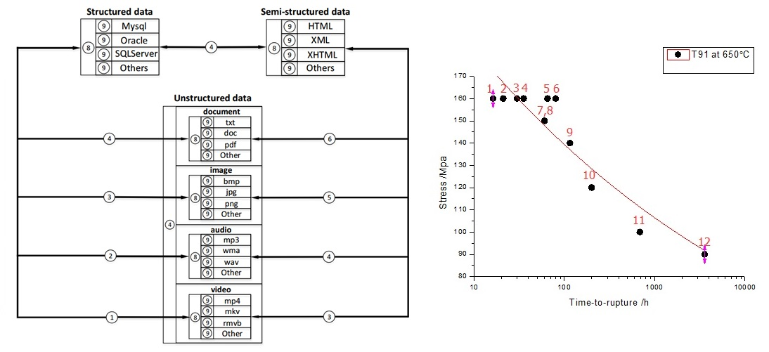
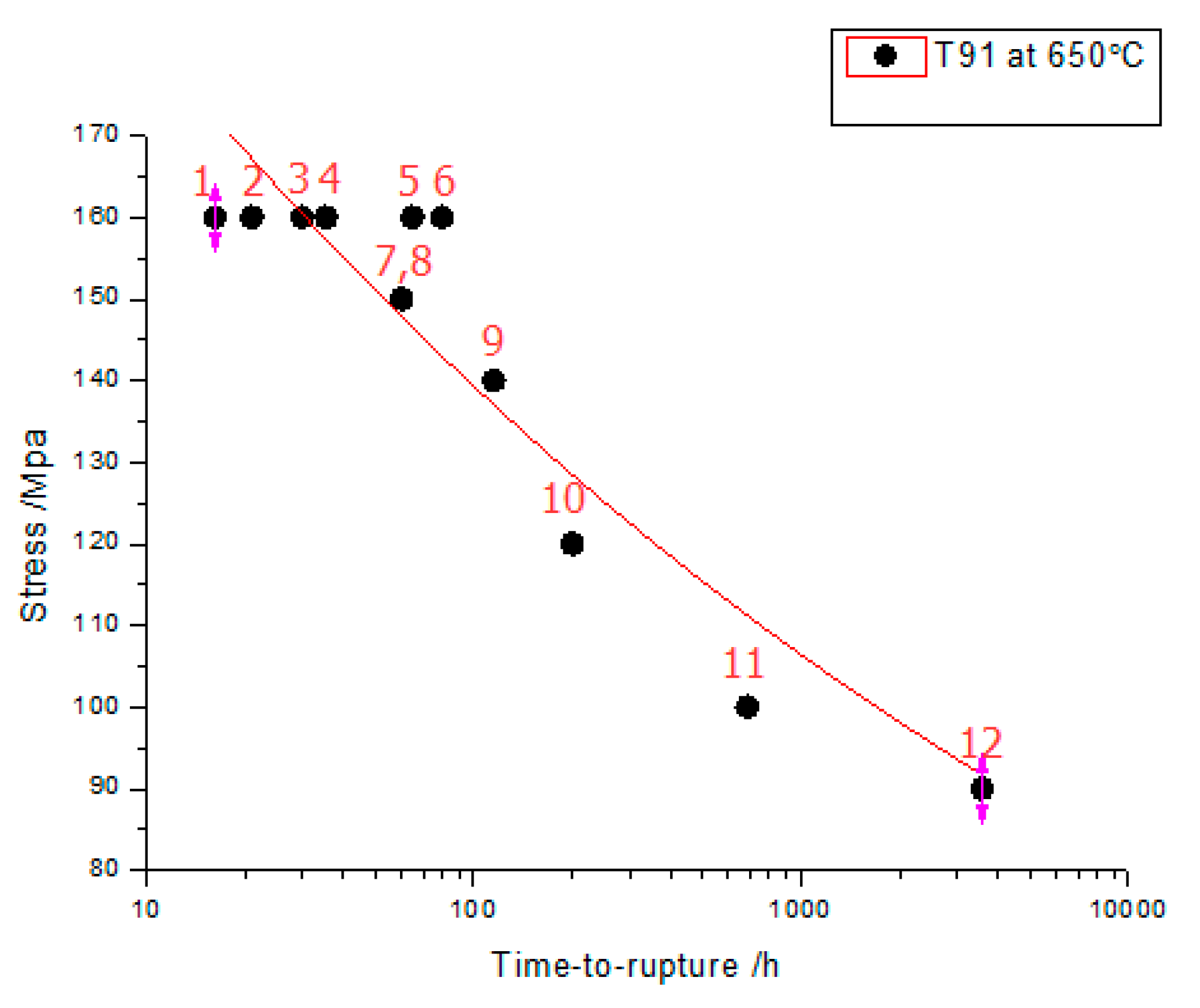
Conditional consistency refers to those which conform to the trend of creep data. Here, creep curve can be seen as the condition. The creep curve in Figure 2 can be more intuitive to analyze data consistency.

As shown in Figure 2, data point 3 is very close to data point 4, so they are consistent. Data point 4 is far from data point 5, so they are inconsistent. Data point 7 and data point 8 overlap and they meet the requirement of strong consistency. If the creep curve is used as a condition, the data points 9, 10, 11, and 12 distributed around the fitted curve are conditionally consistent. Conditional consistency requires that the values of two data meet predefined conditional requirements. It is associated with a particular application, and there needs to be clear knowledge on the logical relationships between data. The conditional consistency here indicates that the points 9, 10, 11, and 12 are probably four different values of the same material performance curve.

Table 6. Deviation between two units in Table 5.

Deviation	1	2	3	4	5	6	7	8	9	10	11	12
1	0.00	0.10	0.28	0.40	1.00	1.31	0.89	0.89	1.99	3.70	13.66	72.98
2	0.10	0.00	0.14	0.23	0.70	0.94	0.60	0.60	1.45	2.76	10.43	56.19
3	0.28	0.14	0.00	0.06	0.39	0.56	0.32	0.32	0.91	1.81	7.19	39.32
4	0.40	0.23	0.06	0.00	0.28	0.42	0.21	0.21	0.71	1.47	6.00	33.14
5	1.00	0.70	0.39	0.28	0.00	0.18	0.06	0.06	0.58	1.59	7.38	41.87
6	1.31	0.94	0.56	0.42	0.18	0.00	0.23	0.23	0.36	1.25	6.51	37.86
7	0.89	0.60	0.32	0.21	0.06	0.23	0.00	0.00	1.09	2.76	12.63	71.60
8	0.89	0.60	0.32	0.21	0.06	0.23	0.00	0.00	1.39	3.52	16.23	92.24
9	1.99	1.45	0.91	0.71	0.58	0.36	1.09	1.39	0.00	0.93	6.37	38.83
10	3.70	2.76	1.81	1.47	1.59	1.25	2.76	3.52	0.93	0.00	2.62	18.19
11	13.66	10.43	7.19	6.00	7.38	6.51	12.63	16.23	6.37	2.62	0.00	3.16
12	72.98	56.19	39.32	33.14	41.87	37.86	71.60	92.24	38.83	18.19	3.16	0.00

shows the deviations between two units in Table 5. Each pair of data units with the same testing condition is treated by Equation (2). In Table 6, 0.10 in the first row and second column is the calculation result of Formula (4). It can be seen that the data in the table is symmetric, which is caused by the symmetric property of data consistency. Larger deviation means larger error between two data units.

Table 7. Consistency degree and relationships of the data in Table 5.

Data Point	1	2	3	4	5	6	7	8	9	10	11	12
1	999/C 1	199/W 2	I 3	I	I	I	I	I	I	I	I	I
2	199/W	999/C	I	I	I	I	I	I	I	I	I	I
3	I	I	999/C	499/W	I	I	I	I	I	I	I	I
4	I	I	499/W	999/C	I	I	I	I	I	I	I	I
5	I	I	I	I	999/C	I	499/W	499/W	I	I	I	I
6	I	I	I	I	I	999/C	I	I	I	I	I	I
7	I	I	I	I	499/W	I	999/C	999/C	I	I	I	I
8	I	I	I	I	499/W	I	999/C	999/C	I	I	I	I
9	I	I	I	I	I	I	I	I	Con 4
10	I	I	I	I	I	I	I	I
11	I	I	I	I	I	I	I	I
12	I	I	I	I	I	I	I	I

¹ C represents complete consistency; ² W represents weak consistency; ³ I represents inconsistency; ⁴ Con represents conditional consistency.

shows the consistency degree and relationships of the data in Table 5. There are the relationships of complete consistency, strong consistency, weak consistency, and inconsistency.

The judgment of conditional consistency depends on the domain knowledge and the conditions set ahead. It reflects the degree to which the data obeys the rules.

4. Discussion

From the data consistency theory and case study on creep testing data, we can see the different physical meanings and application areas of different grades of consistency.

Complete consistency requires that all the parameters of data unit and data set are the same. In fact, completely consistent data probably come from the same source. Because the test result is highly affected by the certain specimen and external environment, it is hard to produce the totally same result for two scientific tests.

Strong consistency requires that the data values of two data are the same under the semantic meaning. The two data that conform to strong consistency may have different storage formats and semantic representations, so their direct sources may be different, but the original source of two data likely is the same.

Weak consistency requires the difference of data values of two data within an acceptable error. Weak consistency in scientific testing data is common. Testing data is influenced by various factors and data collected from different sources has different parameters, so the trend of similar data can be compared through collecting the same kind of material and the same performance data.

Conditional consistency requires that the values of two data meet predefined conditional requirements. It is associated with a particular application, and there needs to be clear knowledge on the logical relationships between data.

The data consistency theory proposed in this paper can effectively evaluate the quality of scientific big data from various sources. It provides a good theoretical foundation for sample data screening of data analysis and data mining.

5. Conclusions

This paper analyzes the causes of the inconsistency phenomenon in scientific big data and proposes data consistency theory for scientific big data. In order to describe the level of consistency, data consistency is divided into complete consistency, strong consistency, weak consistency, and conditional consistency. To evaluate the data quality, the quantitative calculating method of consistency degree is presented. The case study on material creep testing data shows that the theory can evaluate the quality of data. It can be expected that the theory and evaluating method can improve the further application of big data.

The data consistency theory in this paper is only a preliminary system and needs further investigation. Future work will focus on the consistency evaluation of data sets. Another important issue is to study the best consistency degree calculating method. The implementation of the theory and method will be further modified to solve the challenges of the big data age.

References

1. Li, S.; Dragicevic, S.; Anton, F.; Sester, M.; Winter, S.; Coltekin, A.; Pettit, C.; Jiang, B.; Haworth, J.; Stein, A.; et al. Geospatial big data handling theory and methods: A review and research challenges. ISPRS J. Photogramm. Remote Sens. 2016, 115, 119–133. [Google Scholar] [CrossRef] [Green Version]
2. Ishwarappa; Anuradha, J. A Brief Introduction on Big Data 5Vs Characteristics and Hadoop Technology. Procedia Comput. Sci. 2015, 48, 319–324. [Google Scholar] [CrossRef] [Green Version]
3. Gandomi, A.; Haider, M. Beyond the hype: Big data concepts, methods, and analytics. Int. J. Inf. Manag. 2015, 35, 137–144. [Google Scholar] [CrossRef] [Green Version]
4. Fortier, P.J.; Michel, H.E. Database Systems Performance Analysis. In Computer Systems Performance Evaluation and Prediction; Digital Press; Elsevier Science: Amsterdam, The Netherlands, 2003; pp. 409–444. [Google Scholar]
5. Tosun Umut. Distributed Database Design: A Case Study. Procedia Comp. Sci. 2014, 37, 447–450. [Google Scholar] [CrossRef] [Green Version]
6. Gao, H.; Duan, Y.; Miao, H.; Yin, Y. An Approach to Data Consistency Checking for the Dynamic Replacement of Service Process. IEEE Access 2017, 5, 11700–11711. [Google Scholar] [CrossRef]
7. Zhu, Y.; Wang, J. Client-centric consistency formalization and verification for system with large-scale distributed data storage. Future Gener. Comput. Syst. 2010, 26, 1180–1188. [Google Scholar] [CrossRef]
8. Chihoub, H.E. Managing Consistency for Big Data Applications: Tradeoffs and Self-Adaptiveness; Databases [cs.DB]; École Normale Supérieure de Cachan-ENS Cachan: Paris, France, 2013. (In English) [Google Scholar]
9. Liu, J.; Li, J.; Li, W.; Wu, J. Rethinking big data: A review on the data quality and usage issues. ISPRS J. Photogramm. Remote Sens. 2016, 115, 134–142. [Google Scholar] [CrossRef]
10. Gorton, I.; Klein, J. Distribution, data, deployment: Software architecture convergence in big data systems. IEEE Softw. 2015, 32, 78–85. [Google Scholar] [CrossRef]
11. Karger, D. Consistent hashing and random trees: Distributed caching protocols for relieving hot spots on the World Wide Web. ACM Symp. Theory Comput. 1997, 97, 654–663. [Google Scholar]
12. Albanese, M.; Erbacher, R.F.; Jajodia, S.; Molinaro, C.; Persia, F.; Picariello, A.; Sperlì, G.; Subrahmanian, V.S. Recognizing unexplained behavior in network traffic. Netw. Sci. Cybersecur. 2014, 55, 39–62. [Google Scholar]
13. Schutt, T.; Schintke, F.; Reinefeld, A. Structured Overlay without Consistent Hashing: Empirical Results. In Proceedings of the IEEE International Symposium on Cluster Computing and the Grid, Singapore, 16–19 May 2006. [Google Scholar]
14. Flora, A.; Vincenzo, M.; Antonio, P.; Giancarl, S. Diffusion Algorithms in Multimedia Social Networks: A preliminary model. In Proceedings of the 2017 IEEE/ACM International Conference on Advances in Social Networks Analysis and Mining, Sydney, Australia, 31 July–3 August 2017; pp. 844–851. [Google Scholar]
15. Liu, D.; Xu, W.; Du, W.; Wang, F. How to Choose Appropriate Experts for Peer Review: An Intelligent Recommendation Method in a Big Data Context. Data Sci. J. 2015, 14, 16. [Google Scholar] [CrossRef]
16. Pang, L.Y.; Zhong, R.Y.; Fang, J.; Huang, G.Q. Data-source interoperability service for heterogeneous information integration in ubiquitous enterprises. Adv. Eng. Inform. 2015, 29, 549–561. [Google Scholar] [CrossRef]
17. Hinz, K.L.; Mcgee, H.M.; Huitema, B.E.; Dickinson, A.M.; Van Enk, R.A. Observer accuracy and behavior analysis: Data collection procedures on hand hygiene compliance in a neurovascular unit. Am. J. Infect. Control 2014, 42, 1067–1073. [Google Scholar] [CrossRef]
18. Laure, E.; Vitlacil, D. Data storage and management for global research data infrastructures—Status and perspectives. Data Sci. J. 2013, 12, GRDI37–GRDI42. [Google Scholar] [CrossRef]
19. Jiang, D. The electronic data and retrieval of the secret history of the mongols. Data Sci. J. 2007, 6, S393–S399. [Google Scholar] [CrossRef]
20. Aswathy, R.K.; Mathew, S. On different forms of self similarity. Chaos Solitons Fractals 2016, 87, 102–108. [Google Scholar] [CrossRef]
21. Finney, K. Managing antarctic data-a practical use case. Data Sci. J. 2015, 13, PDA8–PDA14. [Google Scholar] [CrossRef]
22. Martínez-Rocamora, A.; Solís-Guzmán, J.; Marrero, M. LCA databases focused on construction materials: A review. Renew. Sustain. Energy Rev. 2016, 58, 565–573. [Google Scholar] [CrossRef]
23. Yao, T.; Kong, X.; Fu, H.; Tian, Q. Semantic consistency hashing for cross-modal retrieval. Neurocomputing 2014, 193, 250–259. [Google Scholar] [CrossRef]
24. Thorsen, H.V. Computer-Implemented Control of Access to Atomic Data Items. U.S. Patent 6052688A, 18 April 2000. [Google Scholar]
25. Yang, S.; Ling, X.; Zheng, Y.; Ma, R. Creep life analysis by an energy model of small punch creep test. Mater. Des. 2016, 91, 98–103. [Google Scholar] [CrossRef]
26. Beliakov, G.; Pagola, M.; Wilkin, T. Vector valued similarity measures for Atanassov’s intuitionistic fuzzy sets. Inf. Sci. 2016, 280, 352–367. [Google Scholar] [CrossRef]
27. He, Y.; Xu, M.; Chen, X. Distance-based relative orbital elements determination for formation flying system. Acta Astronaut. 2016, 118, 109–122. [Google Scholar] [CrossRef]
28. Li, P.F.; Zhu, Q.M.; Zhou, G.D. Using compositional semantics and discourse consistency to improve Chinese trigger identification. Inf. Process. Manag. 2014, 50, 399–415. [Google Scholar] [CrossRef]
29. WordNet. Available online: https://wordnet.princeton.edu (accessed on 8 April 2019).
30. Tongyici Cilin (Extended). Available online: http://www.bigcilin.com/browser/ (accessed on 8 April 2019).
31. Vera-Baquero, A.; Colomo-Palacios, R.; Molloy, O. Real-time business activity monitoring and analysis of process performance on big-data domains. Telemat. Inf. 2016, 33, 793–807. [Google Scholar] [CrossRef]
32. Yurechko, M.; Schroer, C.; Wedemeyer, O.; Skrypnik, A.; Konys, J. Creep-to-rupture of 9% Cr steel T91 in air and oxygen-controlled lead at 650 °C. In Proceedings of the NuMat 2010 Conference, Karlsruhe, Germany, 4–7 October 2010. [Google Scholar]
33. NIMS Database. Available online: https://smds.nims.go.jp/creep/index_en.html (accessed on 8 April 2019).
Figure 1. The calculation rule of Cf value.
Information 10 00137 g001
Figure 2. Creep curve of T91 at 650 °C.
Information 10 00137 g002