Article

Predict Electric Power Demand with Extended Goal Graph and Heterogeneous Mixture Modeling

Faculty of Computer Science and Systems Engineering, Kyushu Institute of Technology, 680-4, Kawazu, Iizuka, Fukuoka 820-8502, Japan
*
Author to whom correspondence should be addressed.
Information 2019, 10(4), 134; https://doi.org/10.3390/info10040134
Submission received: 29 January 2019 / Revised: 4 April 2019 / Accepted: 8 April 2019 / Published: 10 April 2019
(This article belongs to the Special Issue MoDAT: Designing the Market of Data)

Abstract

:
In this study, methods for predicting energy demand on hourly consumption data are established for realizing an energy management system for buildings. The methods consist of an energy prediction algorithm that automatically separates the datasets to partitions (gate) and creates a linear regression model (local expert) for each partition on the heterogeneous mixture modeling, and an extended goal graph that extracts candidates of variables both for data partitioning and for linear regression for the energy prediction algorithm. These methods were implemented as tools and applied to create the energy prediction model on two years’ hourly consumption data for a building. We validated the methods by comparing accuracies with those of different machine learning algorithms applied to the same datasets.

1. Introduction

There is a growing interest in introducing energy management systems in buildings to reduce greenhouse gas emissions [1]. Improving energy efficiency is often described as “low hanging fruit” for reducing the requisite greenhouse gas emissions [2]. The infrastructure for realizing building energy management systems, e.g., field network, standardized protocol for the systems, is already fixed [3]. Nevertheless, the penetration of the systems is far behind the progress of the infrastructure due to lack of building energy modeling [4], which is a crucial tool for predicting power demand and developing informed decisions for reducing energy in buildings.
There are two general types of models for predicting power demands: “linear” and “non-linear” models. In the respect of accuracy in energy prediction, the model extracted from the “non-linear” techniques, e.g., Feed Forward Neural Network (FFNN) [5], and Support Vector Machine (SVM) [6], generally achieves high accuracy. The model extracted from “linear” technique, e.g., Piecewise Liner Regression (PLR) [7], sometimes fails to achieve high enough accuracy, because the “linear” modeling requires explicit domain knowledge about the particular application area for applying. In the building energy modeling, highly interpretable representation becomes also a crucial factor for choosing prediction method [4], because engineers or the energy management system should develop informed decisions for determining an appropriate energy conservation method based on the model. The “linear” model has important advantages over the “non-linear” models in this respect.
We tried to establish methods for predicting power demand on hourly consumption data with the “linear” modeling technique. The methods consist of an energy prediction algorithm that automatically separates the datasets to partitions (gate) and creates a linear regression model (local expert) for each partition on the Heterogeneous Mixture Modeling (HMM) [8,9,10], and an Extended Goal Graph (EGG) [11,12] that extracts candidates of variables both for data partitioning and for linear regression in the HMM algorithm. These methods were implemented as tools and applied to create the energy prediction model on two years’ hourly consumption data for a building.
We validated these methods by comparing accuracies with those of different machine learning algorithms applied to the same datasets. The result was that we confirmed that the EGG tool was succeeded in extracting all-inclusive variables for the gates and the experts, and the energy prediction tool on the HMM created the accurate prediction model by choosing appropriate variables from the candidates without the explicit domain knowledge.

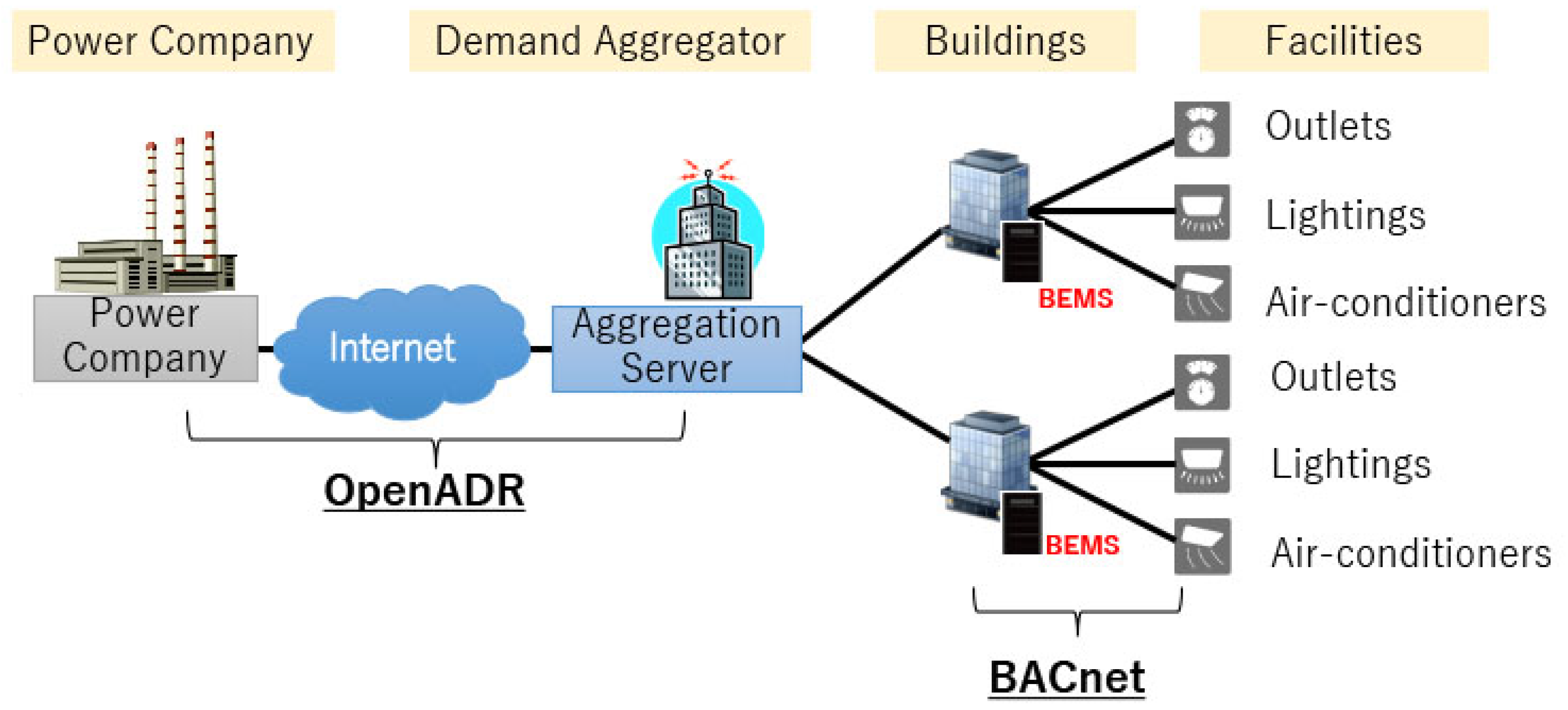
2. Overviews of Building Energy Management System and Energy Demand Prediction Methods

Figure 1 depicts the configuration of a demand management system for buildings. In the system, a Building Energy Management System (BEMS) manages facilities (outlets, lightings, and air conditioners) equipped in each building. The facilities’ management data including hourly power consumption for each facility are transmitted from the BEMS to an aggregation server. The aggregation server receives demand requests from a power company in arbitrary timing and creates demand management plans based on the demand time and the demand value included in the above requests from the power company. Thereafter, the aggregation server orders each BEMS to reduce energy consumption based on the plans and the BEMS controls the facilities for satisfying the plans.
The interface protocol between the power company and the aggregation server is standardized as OpenADR protocol [13] and the interface between the BEMS and the facilities is also standardized as BACnet protocol [14]. For controlling facilities in each building, several kinds of facility control systems were already commercialized as facility control subsystems, e.g., HVAC (Heating, Ventilation, and Air Conditioning) control subsystem, lighting control subsystem, by each facilities’ manufacturer.
The infrastructure for realizing building energy management systems already exists. Nevertheless, the penetration of the systems is far behind the progress of the infrastructure, due to lack of building energy modeling. The building energy modeling is a crucial technique for predicting power demand and developing informed plans for reducing energy consumption without wasteful control actions, which often deteriorate the comfortability and productivity of residents in buildings [15]. Therefore, an accurate and interpretable demand forecasting technique is required for making the demand management plans in the aggregation server so as to reduce wasteful control actions for the facilities equipped in the buildings.

3. Issues and Solutions for Energy Prediction Technique

In recent years, several approaches to establish the energy prediction technique have been considered. As already mentioned in Section 1, these approaches are classified into two groups. One is a group originated from the “linear” regression technique, e.g., multivariate regression [16]. The other is a group that uses a “non-linear” regression technique, e.g., Kernel Machine (KM) [17]. The prediction model extracted from the “non-linear” regression, achieves high predictive performance in comparison with those of “linear” techniques. However, the model from the “non-linear” regression often losses interpretability. The predicted models are utilized as a base for determining control methods of facilities equipped in buildings for reducing energy consumption. Therefore, the model should be easy to be interpreted by engineers and/or the energy management system. The “linear” regression technique has priority compared with the “non-linear” regression technique in this respect.
The partition-wise linear model (PLM) technique [2] was introduced to improve the accuracy in the “linear” regression model. The PLM assigns linear experts to individual partitions on feature space and expresses whole models as patches of local experts. The PLMs have been widely used in many enterprise machine learning problems because it is compact and interpretable representation in terms of both partitions and experts as well as high predictive performance. However, there are two big issues for introducing the PLM into the energy demand prediction in buildings. The first issue is how to extract candidates of variables both for data partitioning (gate) and individual linear regression models (experts) for each gate from huge field data accumulated in the BEMS. The second issue is how to choose appropriate variables for each gate and expert from the candidates without requiring explicit domain knowledge and consuming much processing time.
Support tools to solve the above issues are indispensable for introducing the PLM into the energy demand prediction in buildings. The extended goal graph (EGG) tool helps to extract candidates of variables for the gates and explanatory variables for the experts for each partition from domain experts in building energy management, and the energy prediction (EP) tool on the heterogeneous mixture modeling (HMM) [9,10] realizes to create an accurate prediction model by selecting the most appropriate variables from the candidates extracted in the EGG automatically. The details of these tools are explained in the following sections.

4. Extended Goal Graph (EGG) Tool

The EGG Tool is used to extract candidates of variables for the data partitions and the local experts from the domain engineers’ knowledge. The basic notation methods in the EGG tool are originated from the SysML [18]. The EGG is composed of two planes: a functional structure plane and a data structure plane [12] (Figure 2). The functional structure plane describes the whole structure of the targeted system. In the case of the power demand forecasting in buildings, building facilities like air conditioners (HVAC), lightings, outlets (plug load), are regarded as elements of the functional structure. In each facility, the variables, which affect power consumption for the facility, are enumerated as candidates of variables. For examples, the number of connected devices to the outlet, and operation methods of the device (normally On or Off) are regarded as variables, which affect the power consumption in the outlet. The data structure plane designates data sources and calculation algorithms for providing concrete values to the variables. In the case of the power demand forecasting in buildings, the huge datasets accumulated in BEMS, Security System (SS) and Facility Management System (FMS), are regarded as data sources (Figure 2).
Each data source has datasets, e.g., power consumption at every 30 min in BEMS, the number of passing people of the gate in SS, and average power consumption for each person in FMS. When a variable in the functional structure plane is linked directly to the datasets in the data structure plane, the values to the variable are provided from the datasets in the functional structure plane. When a variable is not obtained directly from the datasets in the data structure plane, the values of the variable are calculated indirectly through a calculation algorithm by combining plural datasets.
For example, “number of person in a room” cannot obtain directly, the values of “number of person in a room” are calculated indirectly from “power consumption at every 30 min” in BEMS, and “average power consumption for each person” in FMS on the ground that the power consumption of outlet is proportional to the number of person in a room (Figure 3). The calculated algorithm is also provided as an element in the data structure plane like the Formula (1):
N u m b e r o f P e r s o n s = P o w e r C o n s u m p t i o n a t e v e r y 30 m i n A v e r a g e p o w e r c o n s u m p t i o n f o r e a c h p e r s o n
The EGG is created through the following steps (Figure 4):
Step1: 
Analyze the functional structure of a targeted system with brainstorming and affinity map [19] among domain engineers (Figure 4 left)
Step2: 
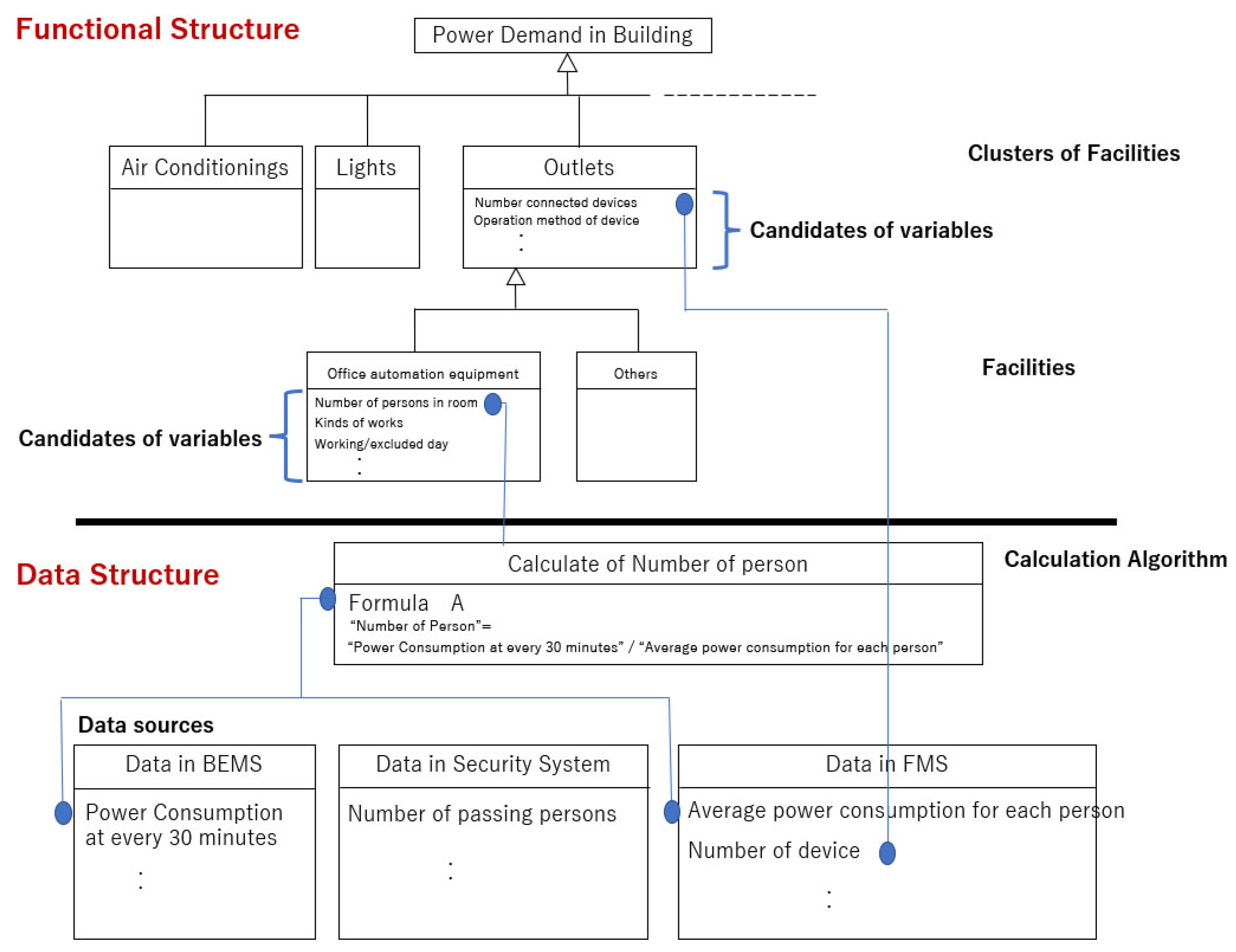
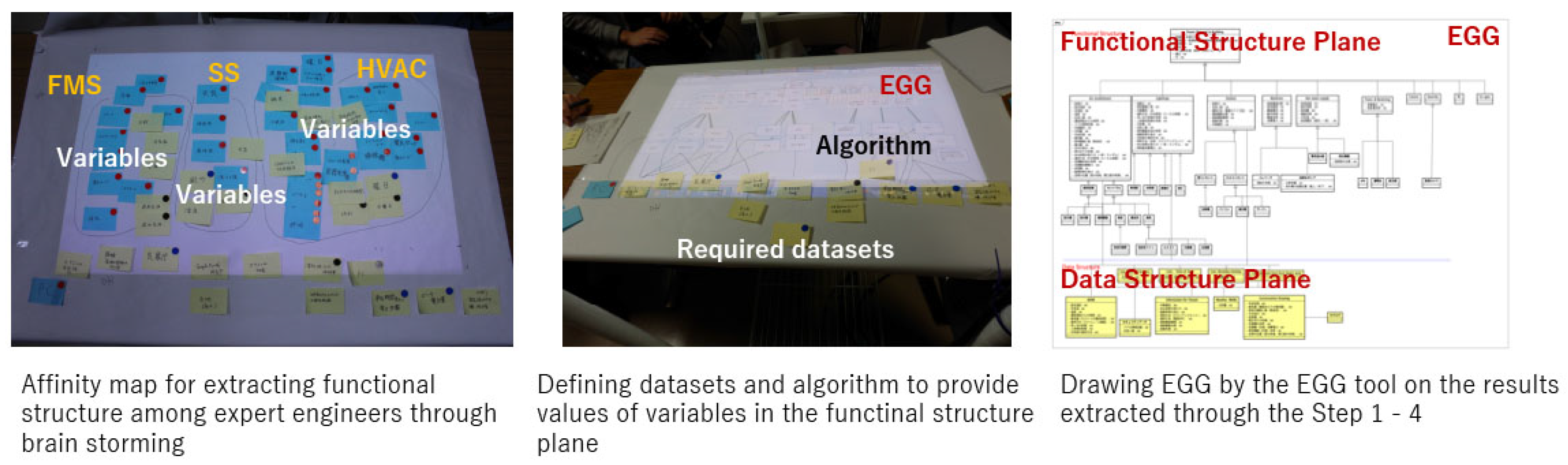
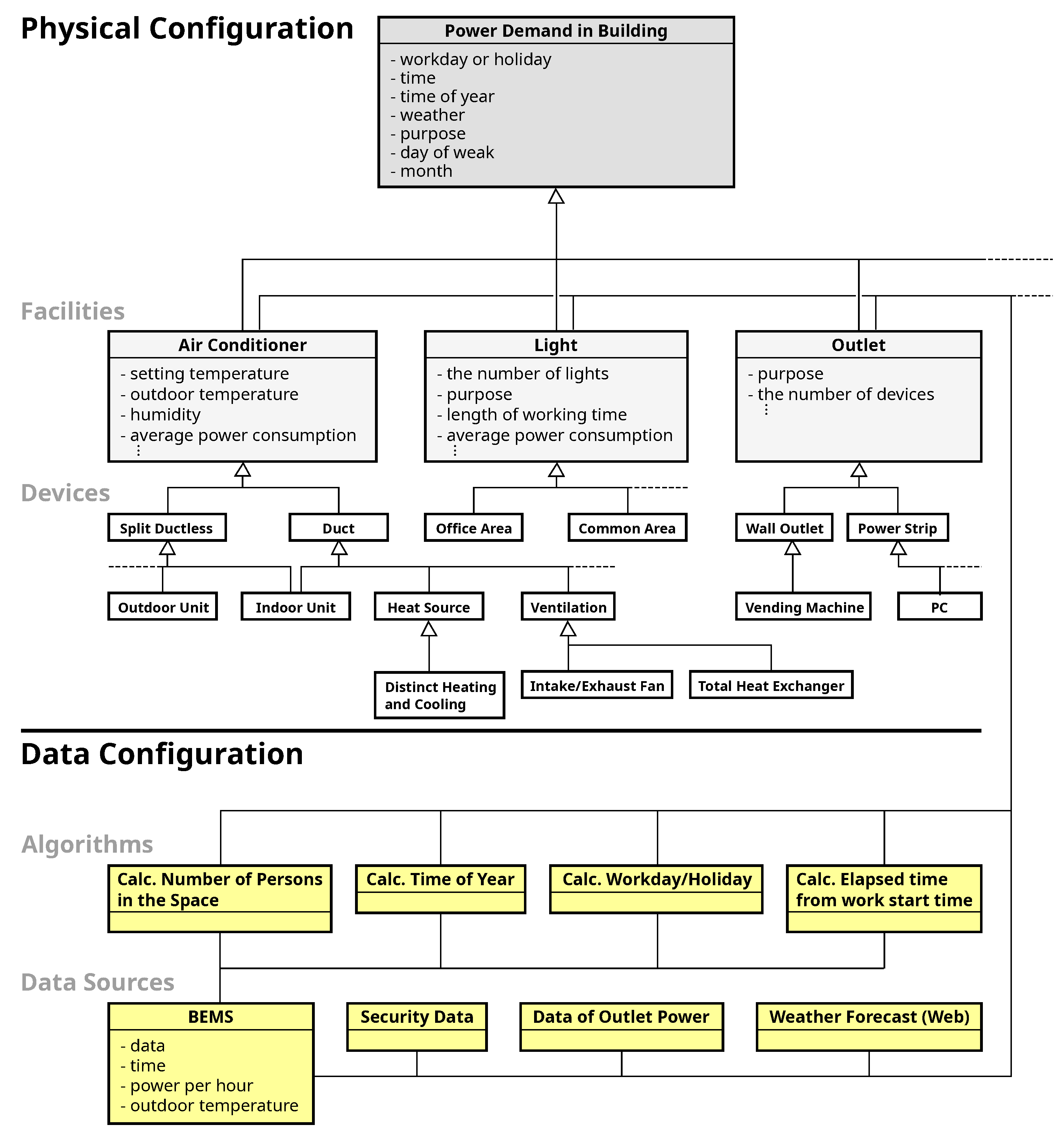
Extract variables to each element in the functional structure plane with brainstorming among domain engineers
Step3: 
Collect required datasets including the variables (Figure 4 middle)
Step4: 
Design algorithm for calculating variables indirectly from raw data included in the above datasets
Step5: 
Draw EGG by using the EGG tool based on the results extracted through Step1–Step4 (Figure 4 right).

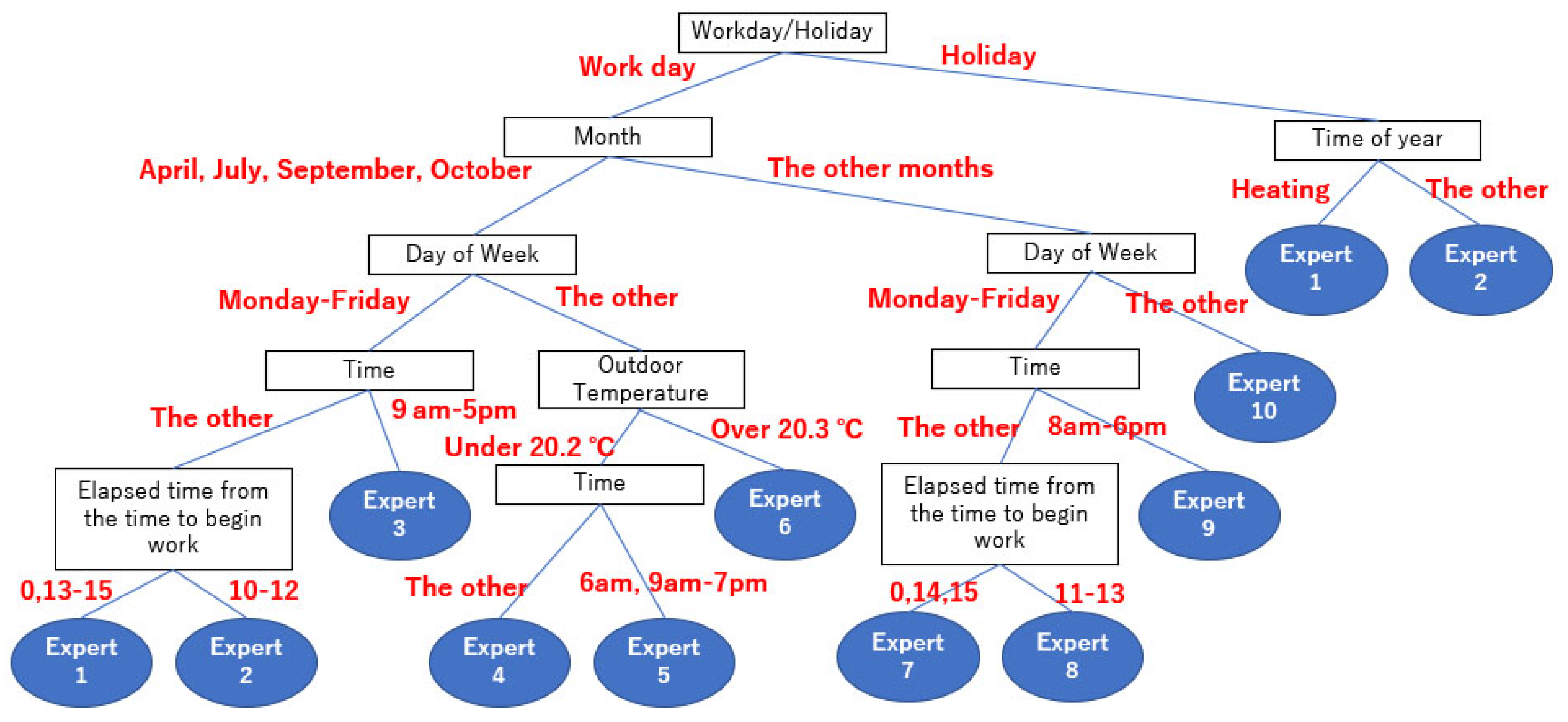
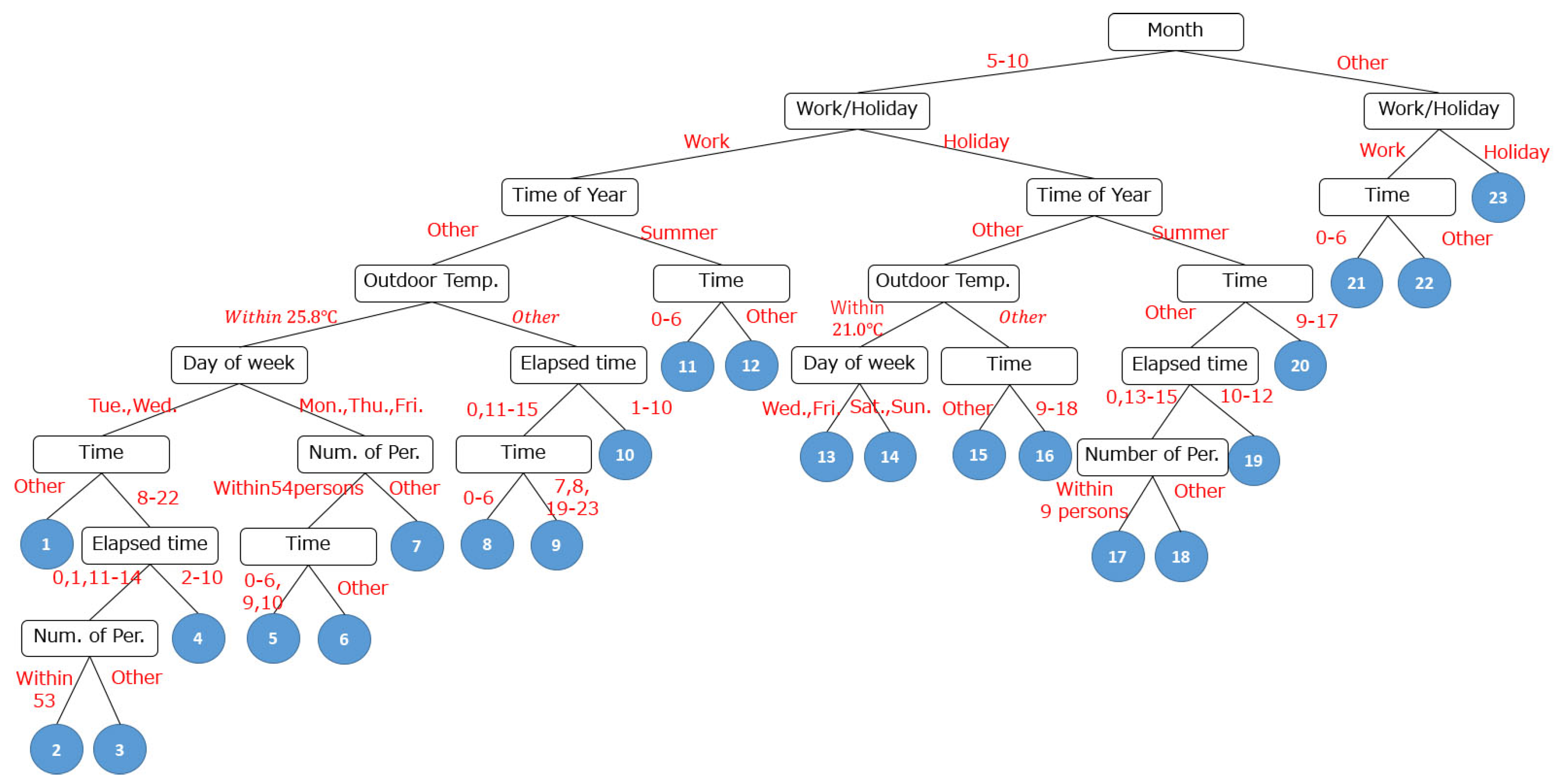
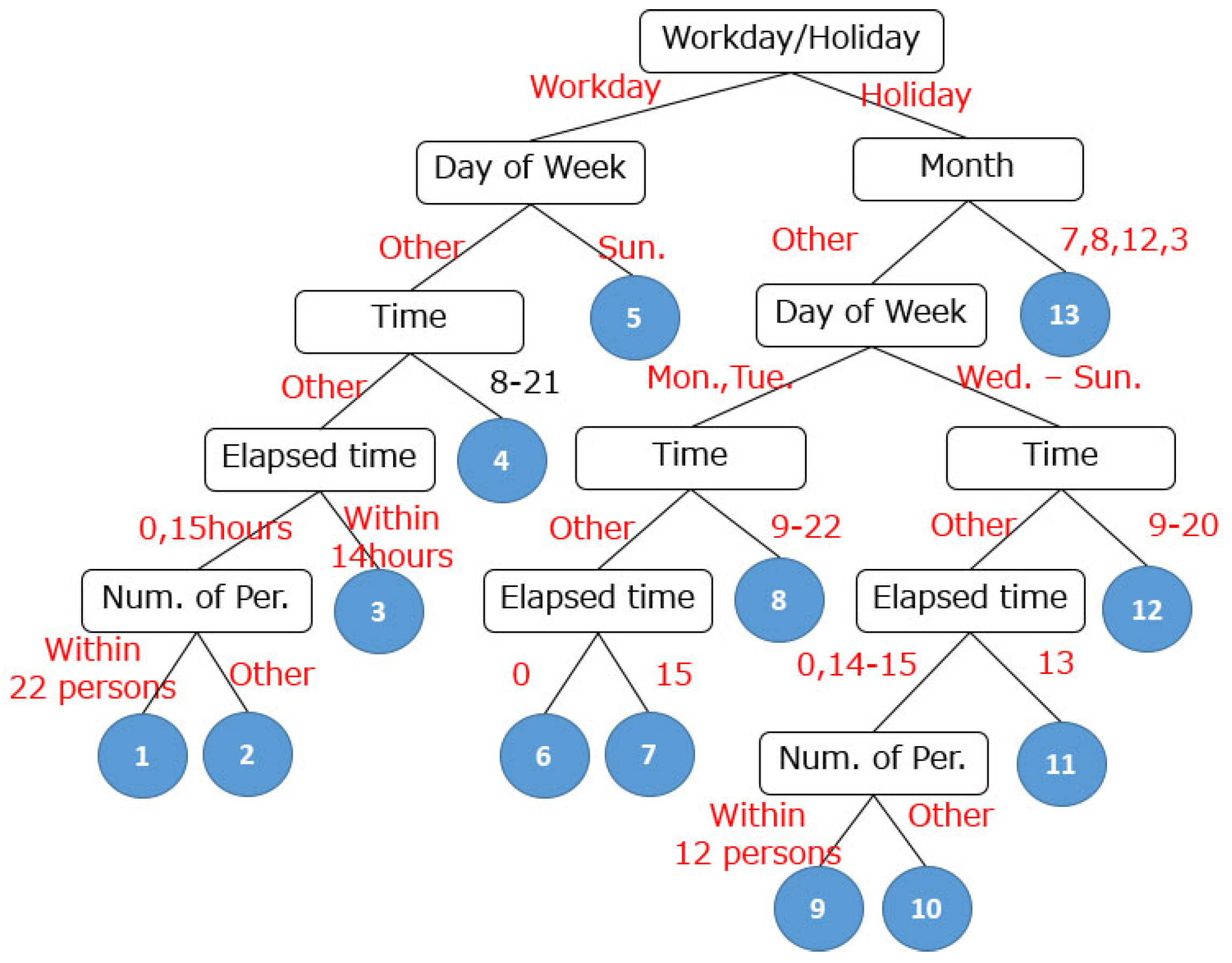
5. Energy Prediction (EP) Tool on the Heterogeneous Mixture Modeling
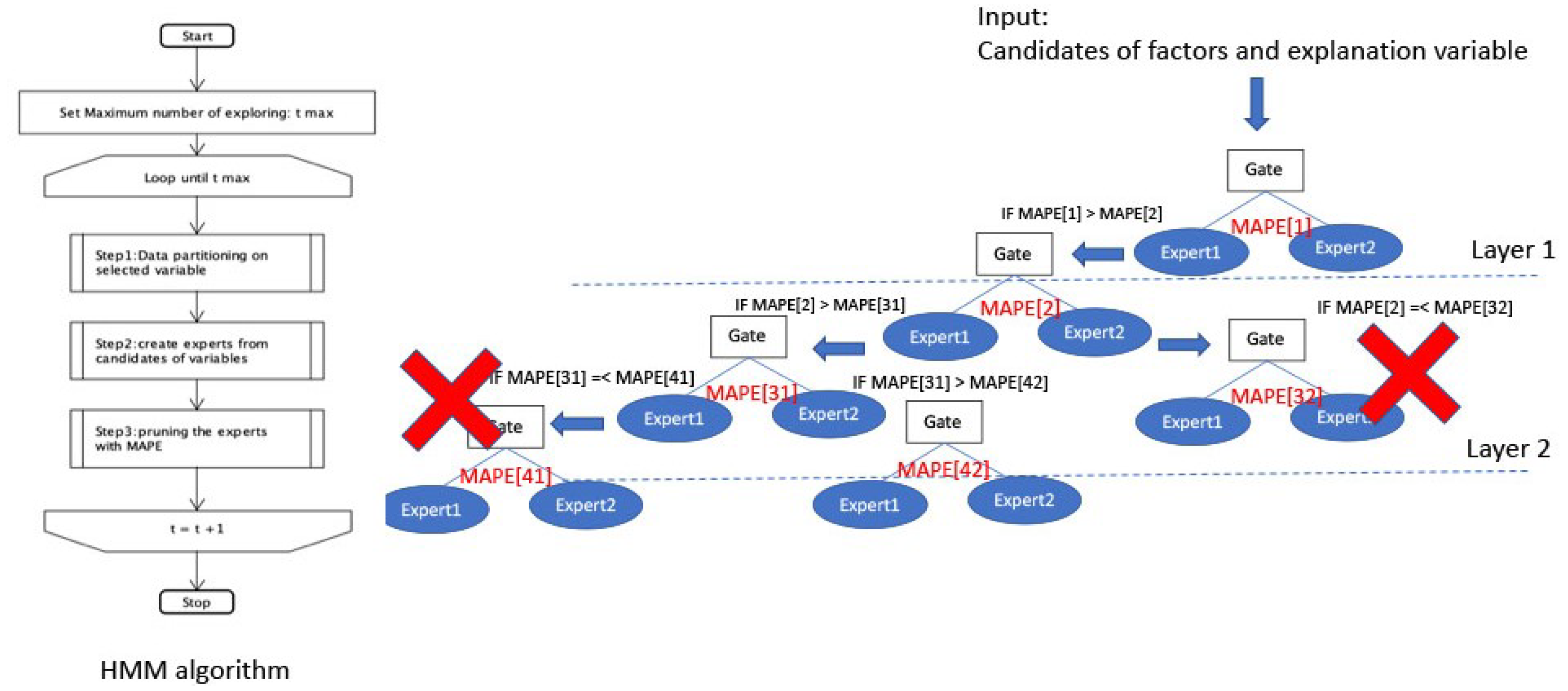
To forecast power demand by the linear regression model, we need to assume factors to divide datasets into partitions and define explanatory variables for linear regression by utilizing our domain knowledge. As a result, the accuracy of the prediction heavily depends on expertise in building energy management and competence in data analysis. In addition, it is quite difficult to improve the accuracy, because it obliges us to use trial and error approach. If factors and explanatory variables for the datasets are enormous, this trial requires much time to execute.
For solving the above problems, the Energy Prediction (EP) tool on the Heterogeneous Mixture Modeling (HMM), that replaces the experts’ trial and error approaches, is developed. The EP tool separates the datasets to appropriate partitions and assigns linear experts for each partition automatically with the candidates of variables defined in the EGG on the HMM algorithm.
The HMM algorithm executes the following three steps recursively to all the candidates of the factors of partitioning and explanatory variables for individual experts (Figure 5):
Step1: 
Select optional factor from the candidates of factors and separate datasets into more than one datasets with the selected factor. The factors, which are used to separate the datasets per each day (e.g., Workday/Holiday) are given priority to the factors used to separate the datasets per every time (e.g., outdoor temperature and the number of people). The interdependency of the divided datasets is validated with the Kruskal-Wallis H-test [20].
Step2: 
Create local experts with candidates of explanatory variables for linear regression and calculate the Mean Absolute Percentage Error (MAPE). The correlation among candidates of variables is checked within the divided datasets. The local experts are created with the independent variables through all search, and the expert which achieves most accurate in the MAPE is selected.
M A P E = 1 n | M e a s u r e d _ V a l u e i P r e d i c t e d _ V a l u e i | M e a s u r e d _ V a l u e i × 100 [ % ]
Step3: 
Pruning the local experts with the MAPE. Select another factor from the candidates and execute Step1 and Step2. If the MAPE for the current expert is less than the MAPE for the previous expert, the algorithm prunes the gate and the local experts.
The algorithm is executed recursively whenever the MAPE of the current expert is improving than the MAPE of the previous expert (Figure 5). When the increase of MAPE in the current expert is less than a threshold, the algorithm prunes the branch and is applied to another branch (Figure 5). As the results of the repetition, the branches (gates) and the leaves (experts) are growing. The EP tool is implemented with R and provides four major functions shown in Table 1.

6. Estimation on the Field Data

We applied the EGG and EP tools to forecast electric demand in a building on two years’ Building Energy Management System’ data. The overview of the datasets for the estimation is shown in Table 2.

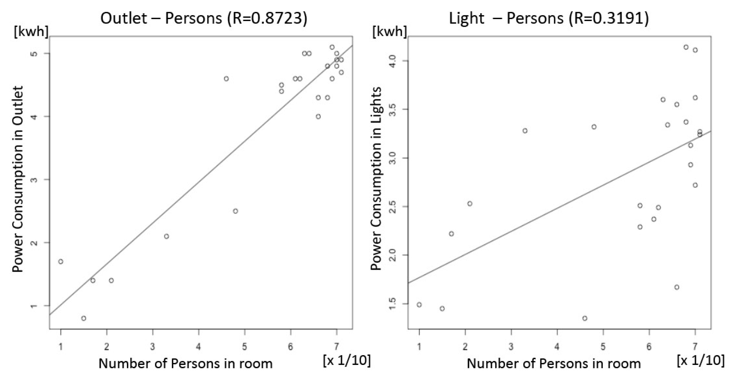
6.1. Extract Candidates for Variables by the EGG Tool

The EGG was created by 6 experts in a BEMS manufacturer through the workshop described in Section 4. As a result, whole facilities (10 facilities class and 31 devices), various factors and variables, and 5 data sources and 4 algorithms required for forecasting the power demand in buildings were configured in the EGG (Figure 7). In the experiment, we selected three major facilities (air-conditioners, lights, and outlets) from ten facilities, and chose eight candidates of factors and variables from the EGG (Table 3).
Each algorithm was inspected its validity on the datasets before using. For example, the algorithm for “Number of Persons in the space” described in Section 4, was validated by comparing the predicted value by the algorithm with the actual value (Figure 8).

6.2. Create Prediction Model by the EP Tool

The EP tool created the energy prediction model from candidates of factors and explanatory variables show in Table 3 automatically and draw the hierarchical structure of factors and local experts. Figure 9 is an example of the prediction model for the outlets of the 5th floor in the building.
Seven variables, workday/holiday, month, day, time, outdoor temp., the elapsed time from the work start time, time of year, are chosen for forecasting energy demand of outlets in 5th floor in the building by the tool. As the results, the datasets are divided into eleven partitions and the experts (linear regression equations) are obtained respectively for each partition (Figure 9). For example, the power demand at 8:00 a.m. Tuesday in April is forecasted by the following equation:
D e m a n d = ( 1.25 × M o n t h ) + ( 0.09 × D a y ) + ( 3.18 × T i m e ) + ( 0.15 × T i m e _ o f _ Y e a r ) + ( 0 × O u t d o o r t e m p . ) + 8.84
We can easily interpret the prediction model by comparing the coefficients of each term in the equation. For example, we understand that the contribution of “Time” and “Month” to the power demand is high because the coefficients of these variables are large. As to air-conditioners and lights, eight variables (all candidates shown in Table 3) are chosen by the EP tool, and datasets are divided into twenty-three (Figure 10) and eights partitions (Figure 11) respectively.

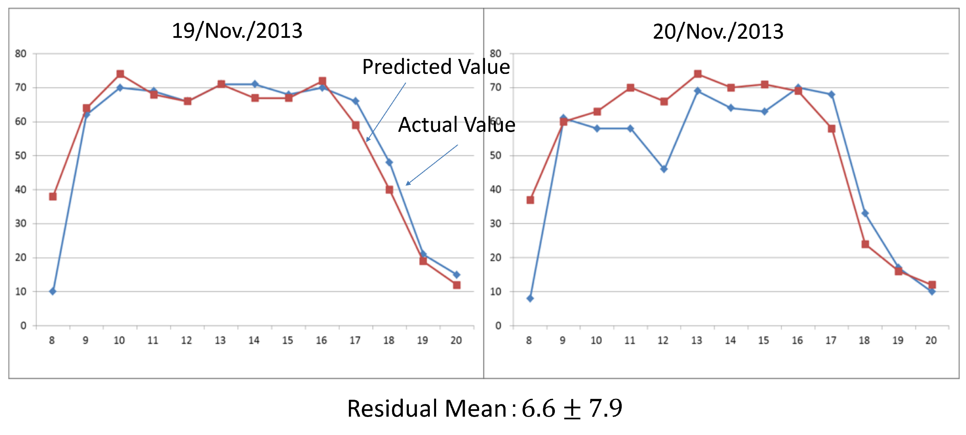
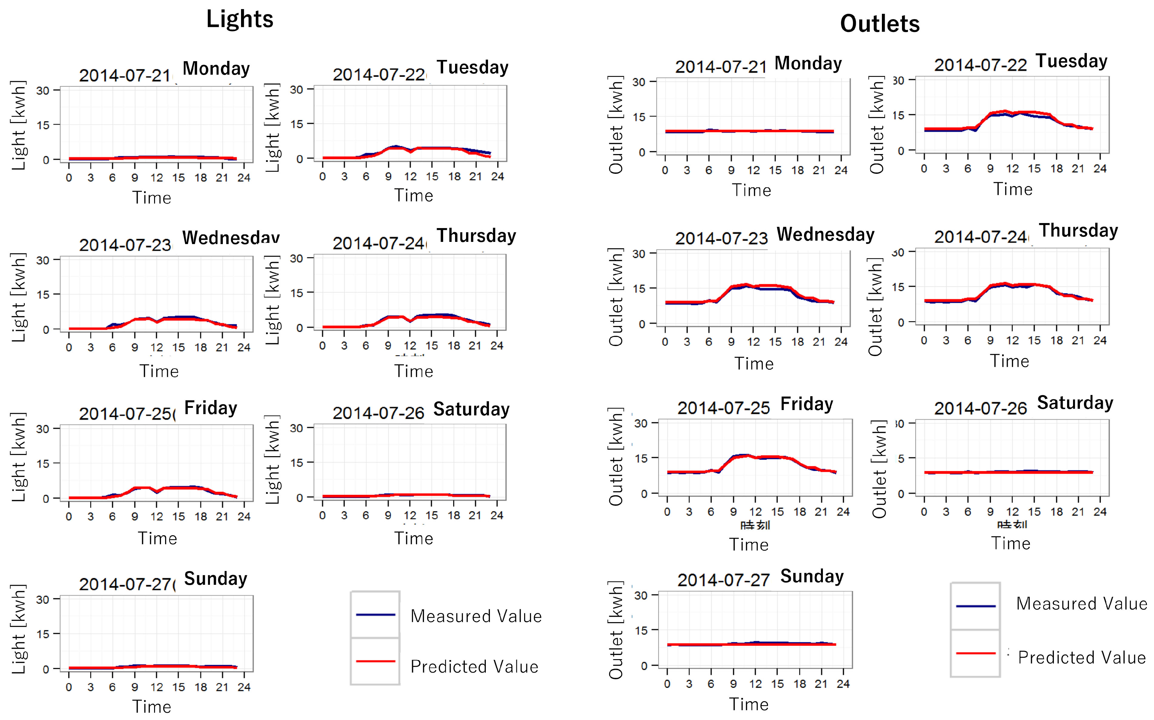
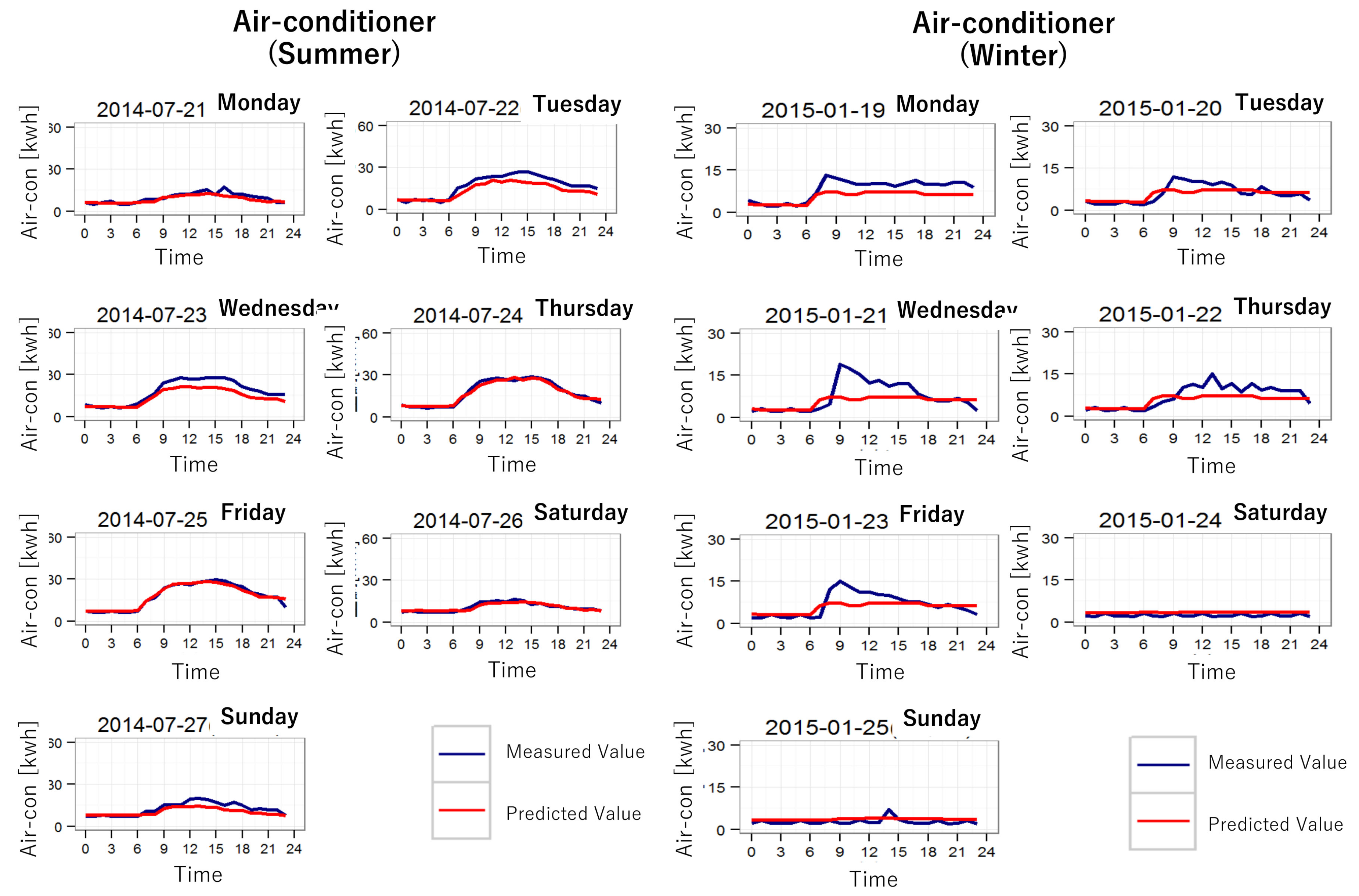
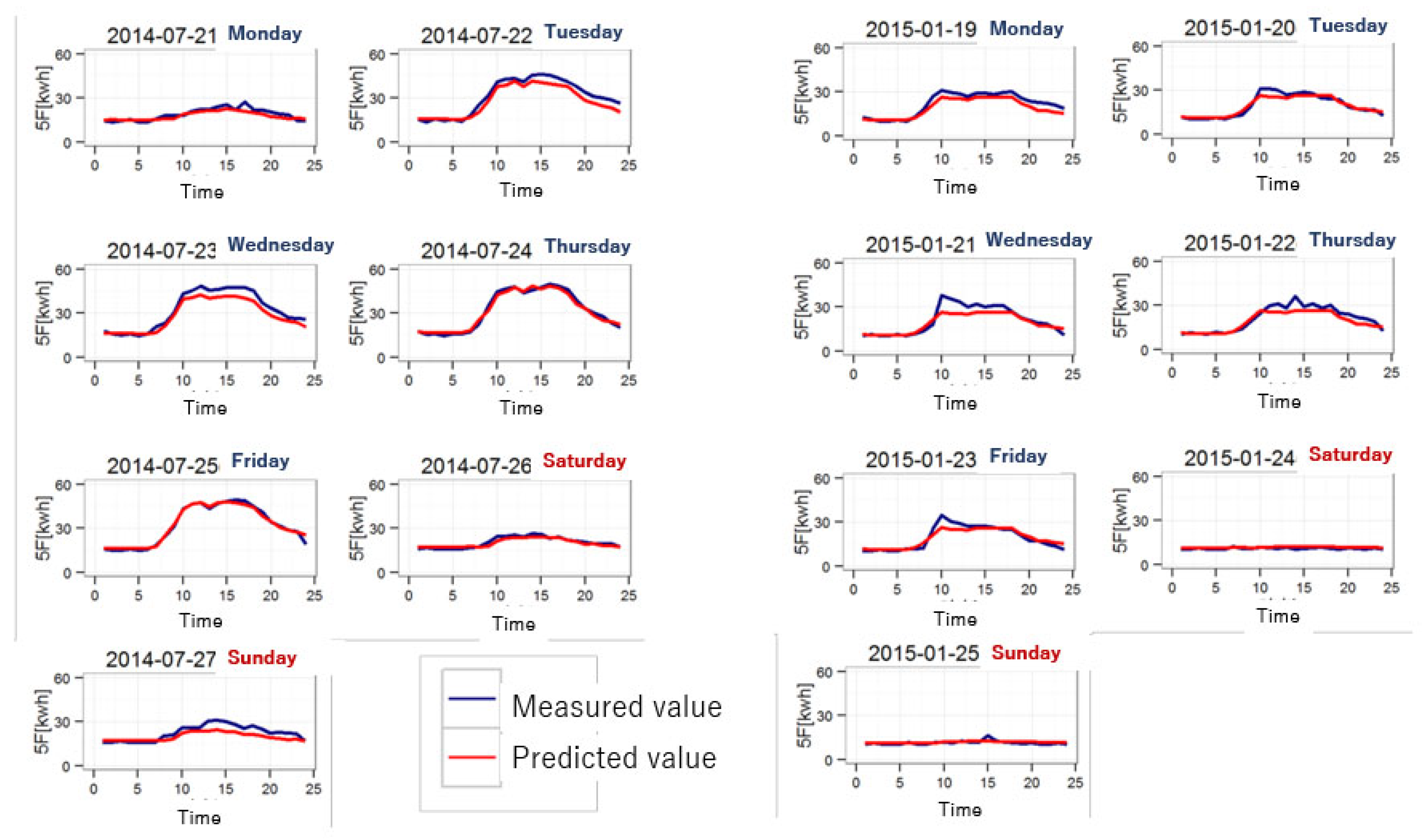
6.3. Results of the Power Demand Forecasting

The models for each facility assign the local experts to individual partitions on feature spaces. The total demand in the building is expressed as patches of the local experts [21]. Therefore, the total demand P t o t a l is calculated by adding the independent models for each facility as the followings:
P t o t a l = P a i r c o n d i t i o n e r s + P l i g h t i n g s + P o u t l e t s
Figure 12 is examples of demand forecasting for lights and outlets by the EP tool and Figure 13 shows the results of demand forecasting for air-conditioners in winter and summer days. Figure 14 is the results of P t o t a l calculated by Equation (3).
We confirm that the EP tool forecasts the power demand accurately on the whole. However, we also discover that the results in the winter morning show a little bad from detail observation in Figure 14. As the prediction model constructed by the EP tool is expressed as a sum of linear terms, we can easily specify error factors of the prediction. In this example, the results for air-conditioners in winter morning (Figure 13) are surmised as a major error factor. The BEMS experts interpret that the residents in the building temporally change the setting temperature of air-conditioning because of low-temperature in these days, and suggest that the results of prediction by the EP tool will be improved by adding new variable “Setting Temperature of Air-conditioners” into the candidates of variables [15].

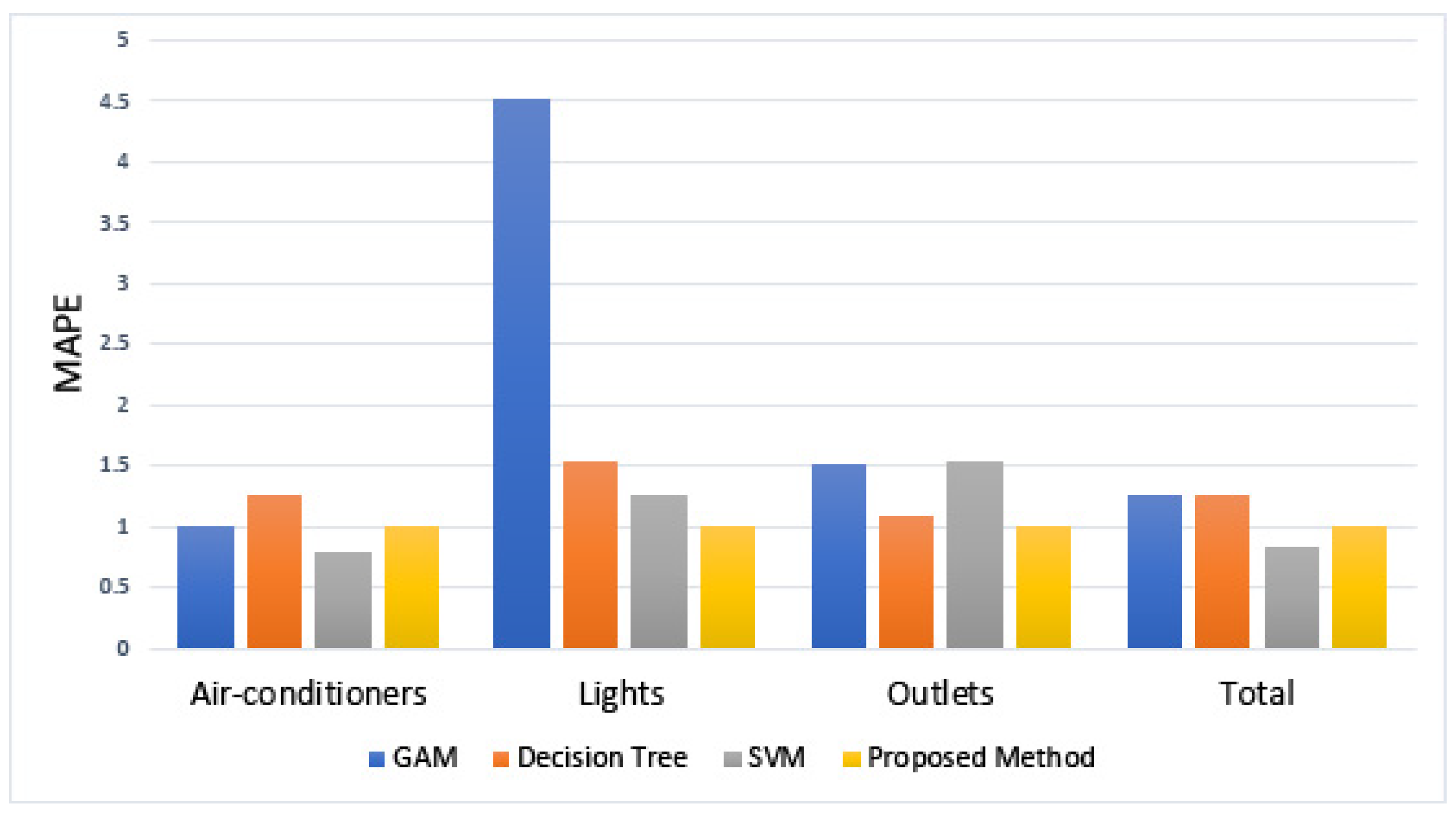
6.4. Comparing Accuracies with the Other Prediction Method

The proposed methods were evaluated by comparing accuracies (MAPE) by those of the other prediction methods. The algorithms on the Generalized Additive Model (GAM) [22], the Decision Tree (DT) [23] and the Support Vector Machine (SVM) [6] are applied to the same datasets shown in Table 2. The GAM is a popular algorithm on linear regression model [24]. All the explanatory variables selected for the GAM (Outdoor temperature, number of people, the elapsed time from the work start time) are quantitative and the relation among power consumption (objective variable) and the explanatory variables (e.g., outdoor temperature) fits exponential distribution, the GAM was selected. The DT is also a popular algorithm on linear regression model [24]. The DT needs not to specify the explanatory variables and users of the DT were not sure which inputs or variables were most beneficial for predicting the specific target. The SVM is a typical algorithm on non-linear regression model and is expected to achieve high accuracy [2].
The results in Table 4 are normalized by the MAPE for the proposed method. The accuracy of the proposed method is better than the other linear regression method and almost equal to the results of the non-linear regression like SVM (Figure 15). As a result of the experiment, we confirm that the extended goal graph tool is succeeded in extracting useful factors and variables both for the gates and the experts, and the energy prediction tool on heterogeneous mixture modeling results in an accurate prediction model by selecting the most appropriate variables from the above candidates automatically.

7. Conclusions

We tried to establish the methods to construct the accurate energy forecast model by introducing the extended goal graph (EGG) and the energy prediction (EP) tool on the heterogeneous mixture modeling (HMM) algorithm. We applied the methods to construct electric power demand models in the building and to estimate the proposed methods with two years’ field data.
The EGG tool was succeeded in extracting useful factors and variables both for the gates and the experts, and the EP tool on HMM algorithm resulted in an accurate prediction model by selecting the most appropriate variables from the candidates of variables obtained in the EGG automatically. The linear regression model elicited from the tools was easy to interpret and useful to define the control method to reduce the energy consumption in the building.
For the future, we plan to develop a demand management system by utilizing these tools and applying the system to real buildings. In this paper, we apply the methods for deriving the energy prediction model from the two years’ field data. However, we think that these methods, the EGG and the prediction algorithm on the HMM, are widely used to the other applications, which are preferred to create interpretable models from big data. By applying these methods to several applications, we would like to improve the methods and put them into practical use in the near feature.

Author Contributions

Conceptualization, N.K.; methodology, N.K., A.F., M.K.; software, A.F. and M.K.; validation, N.K. and T.; formal analysis, N.K., A.F., M.K.; investigation, N.K., A., M.K. and T.M.; resources, T.M.; data curation, T.M.; writing—original draft preparation, N.K. and A.F.; writing—review and editing, N.K.; visualization, N.K., A.F.; supervision, N.K.; project administration, N.K.; funding acquisition, N.K. and T.M.

Funding

This work was partly supported by JST CREST JPMJCR1304.

Conflicts of Interest

The authors declare no conflict of interest.

References

  1. Agency for Natural Resources and Energy in Japan. The 5th Strategic Energy Plan. Available online: https://www.enecho.meti.go.jp/en/ (accessed on 8 April 2019).
  2. Edwardsa, R.E.; Newb, J.; Parker, L.E. Predicting future hourly residential electrical consumption: A machine learning case study. Energy Build. 2012, 49, 591–603. [Google Scholar] [CrossRef]
  3. Mancasi, M.; Vatu, R.; Ceaki, O.; Porumb, R.; Seritan, G. Evolution of smart buildings. A Romanian case. In Proceedings of the 50th International Universities Power Engineering Conference (UPEC), Staffordshire, UK, 1–4 September 2015. [Google Scholar]
  4. Rudin, C. Algorithm for interpretable machine learning. In Proceedings of the 20th ACM SIGKDD Conference on Knowledge Discovery and Data Mining (KDD), New York, NY, USA, 24–27 August 2014. [Google Scholar]
  5. MacKay, D.J. Bayesian nonlinear modeling for the prediction competition. ASHRAE Trans. 1994, 100, 1053–1062. [Google Scholar]
  6. Dong, B.; Cao, C.; Lee, S. Applying support vector machines to predict building energy consumption in tropical region. Energy Build. 2005, 37, 545–553. [Google Scholar] [CrossRef]
  7. Iijima, M.; Takeuchi, R.; Takagi, K.; Matsumoto, T. Piecewise-linear regression on the ASHRAE time-series data. ASHRAE Trans. 1994, 100, 1088–1095. [Google Scholar]
  8. Fujimaki, R.; Sogawa, Y.; Morinaga, S. Online heterogeneous mixture modeling with marginal and copula selection. In Proceedings of the 17th ACM SIGKDD International Conference on Knowledge Discovery and Data Mining, San Diego, CA, USA, 21–24 August 2011. [Google Scholar]
  9. Oiwa, H.; Fujimaki, R. Partition-wise linear models. Adv. Neural Inf. Process. Syst. 2014, 27, 3527–3535. [Google Scholar]
  10. Eto, R.; Fujimaki, R.; Morinaga, S.; Tamano, H. Fully-automatic bayesian piecewise sparse linear models. In Proceedings of the 17th International Conference on Artificial Intelligence and Statistics, Reykjavik, Iceland, 22–24 April 2014. [Google Scholar]
  11. Kushiro, N.; Shimizu, T.; Ehira, T. Requirements elicitation with extended goal graph. In Proceedings of the 20th International Conference on Knowledge Based and Intelligent Information and Engineering System, KES2016, York, UK, 5–7 September 2016; pp. 1691–1700. [Google Scholar]
  12. Ifuku, M.; Kushiro, N.; Aoyama, Y. Requirements definition with extended goal graph. In Proceedings of the IEEE International Conference on Data Mining, Singapore, 17–20 November 2018. [Google Scholar]
  13. OpenARD Alliance. OpenADR2.0 Specifications. Available online: https://www.openadr.org (accessed on 8 April 2019).
  14. ASHRAE. A Data Communication Protocol for Building Automation and Control Networks. Available online: http://www.bacnet.org/Overview/index.html (accessed on 8 April 2019).
  15. Mega, T.; Kitagami, S.; Kawawaki, S.; Kushiro, N. Experimental evaluation of a fast demand response system for small and medium sized office buildings. In Proceedings of the 31st IEEE International Conference on Advanced Information Networking and Application (WAINA2017), Taipei, Taiwan, 27–29 March 2017. [Google Scholar]
  16. Ryan, S.E.; Porth, L.S. A Tutorial on the Piecewise Regression Approach Applied to Bed Load Transport Data; General Technical Report RMRS-GTR-189; US Department of Agriculture, Forest Service, Rocky Mountain Research Station: Fort Collins, CO, USA, 2007. Available online: https://www.fs.usda.gov/treesearch/pubs/all/27004 (accessed on 8 April 2019).
  17. Hofmann, T.; Schlkopf, B.; Smola, A.J. Kernel methods in machine learning. Ann. Stat. 2008, 36, 11711220. [Google Scholar] [CrossRef]
  18. Friedentahl, S.; Moore, A.; Steiner, R. A Practical Guide to SysML; Morgan Kaufmann OMG Press: Needham, MA, USA, 2012. [Google Scholar]
  19. Gray, D.; Brown, S.; Macnufo, J. Game Storming a Playbook for Innovators, Rule Breakers, and Change Makers; O’REILLY: Springfield, MO, USA, 2010. [Google Scholar]
  20. Corder, G.W.; Foreman, D.I. Nonparametric Statistics for Non-Statisticians a Step-by-Step Approach; John Wiley & Sons: Hoboken, NJ, USA, 2009. [Google Scholar]
  21. Porumb, R.; Postolache, P.; Seritan, G.; Vatu, R.; Ceaki, O. Load profiles analysis for electricity market. Comput. Methods Soc. Sci. 2013, 1, 30–38. [Google Scholar]
  22. Hastie, T.J.; Tibshirani, R.J. Generalized Additive Models; Chapman & Hall: Boca Raton, FL, USA, 1990. [Google Scholar]
  23. Kaminski, B.; Jakubczyk, M.; Szufel, P. A framework for sensitivity analysis of decision trees. Cent. Eur. J. Oper. Res. 2017, 26, 135–159. [Google Scholar] [CrossRef] [PubMed] [Green Version]
  24. Lander, J.P. R for Everyone: Advanced Analytics and Graphics; Addison-Wesley: Boston, MA, USA, 2017. [Google Scholar]
Figure 1. Overview of demand management system for buildings.
Information 10 00134 g001
Figure 2. Overview of the Extended Goal Graph (EGG).
Information 10 00134 g002
Figure 3. Relations among number of persons, power consumption in light and outlet.
Information 10 00134 g003
Figure 4. EGG creating process with the brain storming and the affinity map.
Information 10 00134 g004
Figure 5. The algorithm for energy prediction tool on the HMM.
Information 10 00134 g005
Figure 6. Example of visualization of gates and experts by the EP tool.
Information 10 00134 g006
Figure 7. The EGG for building energy prediction.
Information 10 00134 g007
Figure 8. Example of algorithm validation (number of persons).
Information 10 00134 g008
Figure 9. The prediction model for outlets by the tool.
Information 10 00134 g009
Figure 10. The prediction model for air-conditioners by the tool.
Information 10 00134 g010
Figure 11. The prediction model for lights by the tool.
Information 10 00134 g011
Figure 12. Results of the prediction for lights and outlets by the EP tool.
Information 10 00134 g012
Figure 13. Results of the prediction for air-conditioners (summer and winter) by the EP tool.
Information 10 00134 g013
Figure 14. The results of the prediction by the EP tool for 5th floor in summer and winter days.
Information 10 00134 g014
Figure 15. Results of prediction accuracies for prediction methods.
Information 10 00134 g015
Table 1. Function list of the EP tool.
Num.Functions
1Define appropriate prediction model on the learning data with the candidates of factors and explanation variables obtained in the EGG
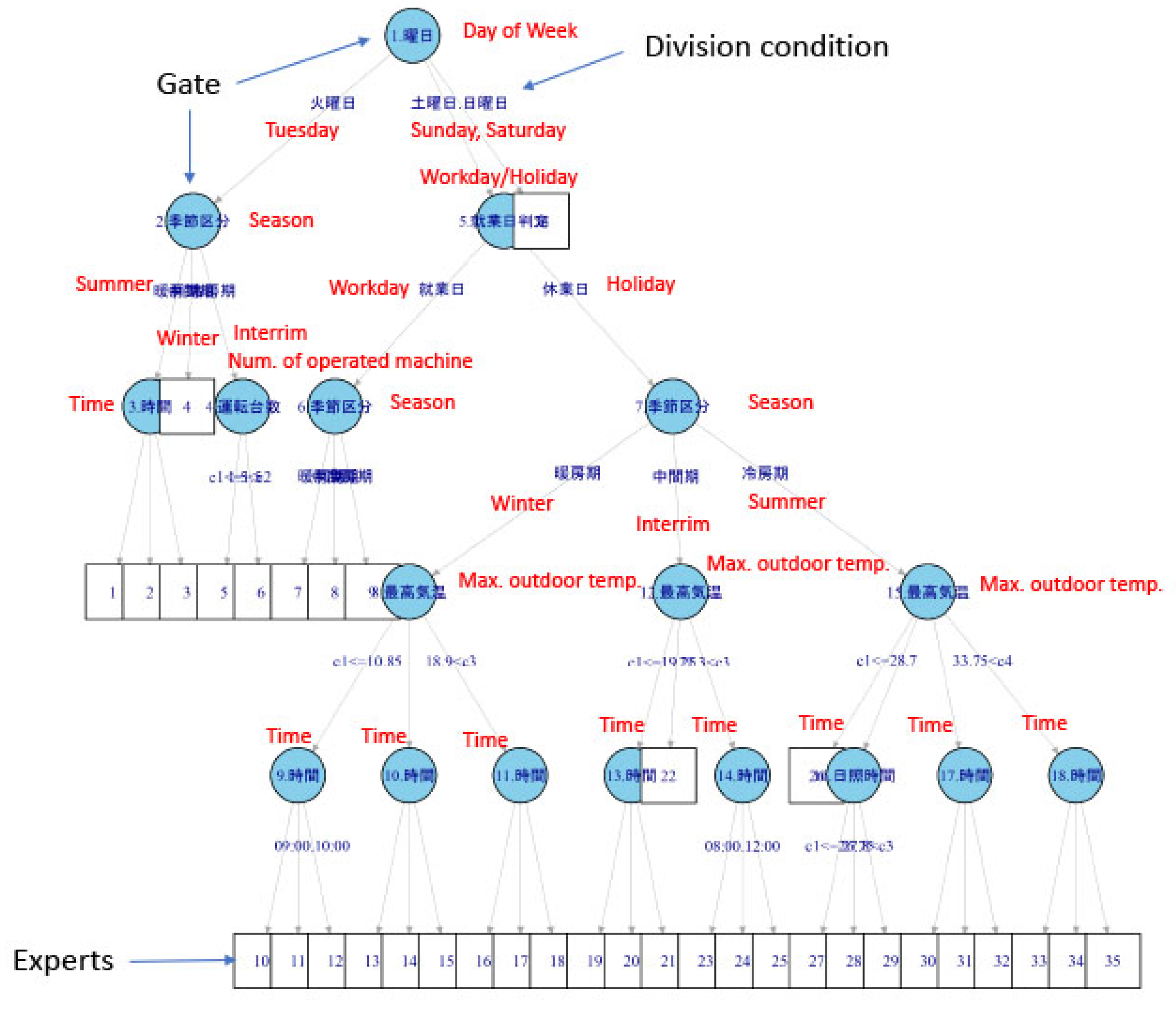
2Visualize hierarchical structure of factors and local experts (Figure 6)
3Predict the energy demand on the testing data
4Calculate MAPE in comparison with the predicted value and the measured value
Table 2. BEMS datasets for the estimation.
ItemDetail
Targeted dataBEMS data for eight stories office building
Data period1 March 2013–31 March 2015 (730 days)
Data for learning1 April 2013–31 March 2014 (365 days)
Data for estimation31 March 2015 (365 days)
Variables included in datasetsdate + time + power per hour + outdoor temperature
File format and SizeCSV (about 8 MB)
Table 3. Candidate for variables for forecasting demand in buildings.
Candidate of VariableSource of Datasets
Workday/HolidayCalculated indirectly with the algorithm on BEMS data
Day of weekBEMS data
TimeBEMS data
Elapsed time the from work start timeBEMS data
MonthBEMS data
Time of year (cooling/heating/the other)Calculated indirectly with the algorithm on BEMS data
Outdoor temperatureBEMS data
Number of people in the spaceCalculated indirectly with the algorithm on BEMS data
Table 4. Comparison prediction accuracies with other algorithm.
MethodsAir-ConditionersLightingsOutletsTotal
Generalized Additive Model (GAM)1.004.541.521.29
Decision Tree1.271.551.091.25
Support Vector Machine (SVM)0.811.261.540.85
Proposed Methods1.001.001.001.00

