Article

Haze Image Recognition Based on Brightness Optimization Feedback and Color Correction

1
Automation College, Beijing University of Posts and Telecommunications, Beijing, 100876, China, [email protected] (S.H.)
2
Beijing Key Laboratory of Control Technology for Toxic, Hazardous, Flammable and Explosive Sources of City, Beijing Municipal Institute of Labor Protection, Beijing, 100054, China
*
Author to whom correspondence should be addressed.
Information 2019, 10(2), 81; https://doi.org/10.3390/info10020081
Submission received: 28 January 2019 / Revised: 19 February 2019 / Accepted: 22 February 2019 / Published: 25 February 2019

Abstract

:
At present, the identification of haze levels mostly relies on traditional measurement methods, the real-time operation and convenience of these methods are poor. This paper aims to realize the identification of haze levels based on the method of haze images processing. Therefore, this paper divides the haze images into five levels, and obtains the high-quality haze images in each level by the brightness correction of the optimization solution and the color correction of the feature matching. At the same time, in order to reduce the noise of the haze images, this article improved the Butterworth filter. Finally, based on the processed haze images, this paper uses the Faster R-CNN network to identify the haze levels. The results of multiple sets of comparison experiments demonstrate the accuracy of the study.

1. Introduction

Nowadays, due to the continuous advancement of urban industrialization, the haze problem has seriously affected the daily life of human beings. The formation of haze can lead to a decrease in visibility, and different levels of haze can cause huge brightness differences and chromatic aberrations in the surrounding environment. In order to effectively and conveniently monitor the severity of haze, the researchers proposed a number of image defogging and enhancement techniques. However, the current research has no suitable solution for the huge interference of brightness and chromatic aberration on the haze images, which seriously affects the accuracy of haze level recognition. Therefore, this paper proposes the correction and recognition of the same ambient haze images based on optimal feedback, aiming to correct the error caused by illumination and imaging conditions in the same environment, and to identify the haze level based on the corrected image.
At present, Lu Lipeng et al. realized the classification and recognition of haze pollution level based on image gray difference statistics [1]. Ji Dabo team achieved the measurement of soot environment by establishing a model of the relationship between image gray value and dust concentration [2]. Zhang Han et al. determined the degree of air pollution by solving the second derivative of image brightness [3]. However, these algorithms are inefficiently identified, and the use of deep learning to identify target images is a more popular and efficient method. For example, Yan Gang et al. used convolutional neural networks (CNN) to identify traffic speed limits in haze environments [4]. Jiang Xiaoping et al. based on recurrent neural network (RNN) to deal with image features in haze environments [5]. However, the interference of the illumination and imaging equipment itself can seriously affect the accuracy of identifying the haze image. At present, people generally solve this problem from two aspects of brightness and color. In solving the difference in image brightness, Wan Mingjie et al. proposed an infrared image enhancement method based on adaptive histogram partition and brightness correction (AHP-BC) [6]. Wang A. et al. used atmospheric illumination prior (AIP) to correct the brightness of the image while maintaining the color of the haze image [7]. Dynamic histogram equalization (DHE) proposed by Abdullah-Al-Wadud et al. tends to preserve the details of the input [8]. Vicker et al. proposed plateau histogram equalization (PHE) to alleviate over-enhancement of illumination, whose probability density function is limited via a threshold [9]. In solving image color differences, Lee Yongho has designed a method for enhancing the accuracy of color correction in stereo images [10]. Karen Panetta proposed two new image multi-color transfer algorithms for still images and image sequences [11]. In addition, some people have corrected based on various image characteristics. Wang Dianwei et al. proposed a multi-spectral image enhancement algorithm based on illuminance-reflection imaging model and morphological operation to correct the brightness and color of the image [12]. Tian Qichong proposed a variation-based fusion method, which obtained enhanced results through a variation-based fusion model via contrast optimization and color correction [13]. In addition to differences in image brightness and color, the image noise will affect the recognition of haze. There are numerous filters to reduce the noise as follows: median of median filter [14], fast bilateral filter [15], and Butterworth filter [16]. The ideal high-pass filter truncates all low-frequency components in the Fourier transform, so the filtered image will have severe ringing effect.
In summary, at present, the identification and classification methods of haze images are insufficiently considered for the huge interference caused by brightness and color. As in the literature [1], only the grayscale histogram of the haze image is classified, which ignored the change in brightness and color in the haze environment. In addition, research on haze images has been focused on achieving defogging of images, ignoring the processing between haze images of the same level. Therefore, for the identification research of haze images, the correction of the luminance difference, and chromatic aberration between images should be considered first, and the noise reduction processing method conforming to the corrected image should be selected, and finally the haze level identification can be realized.
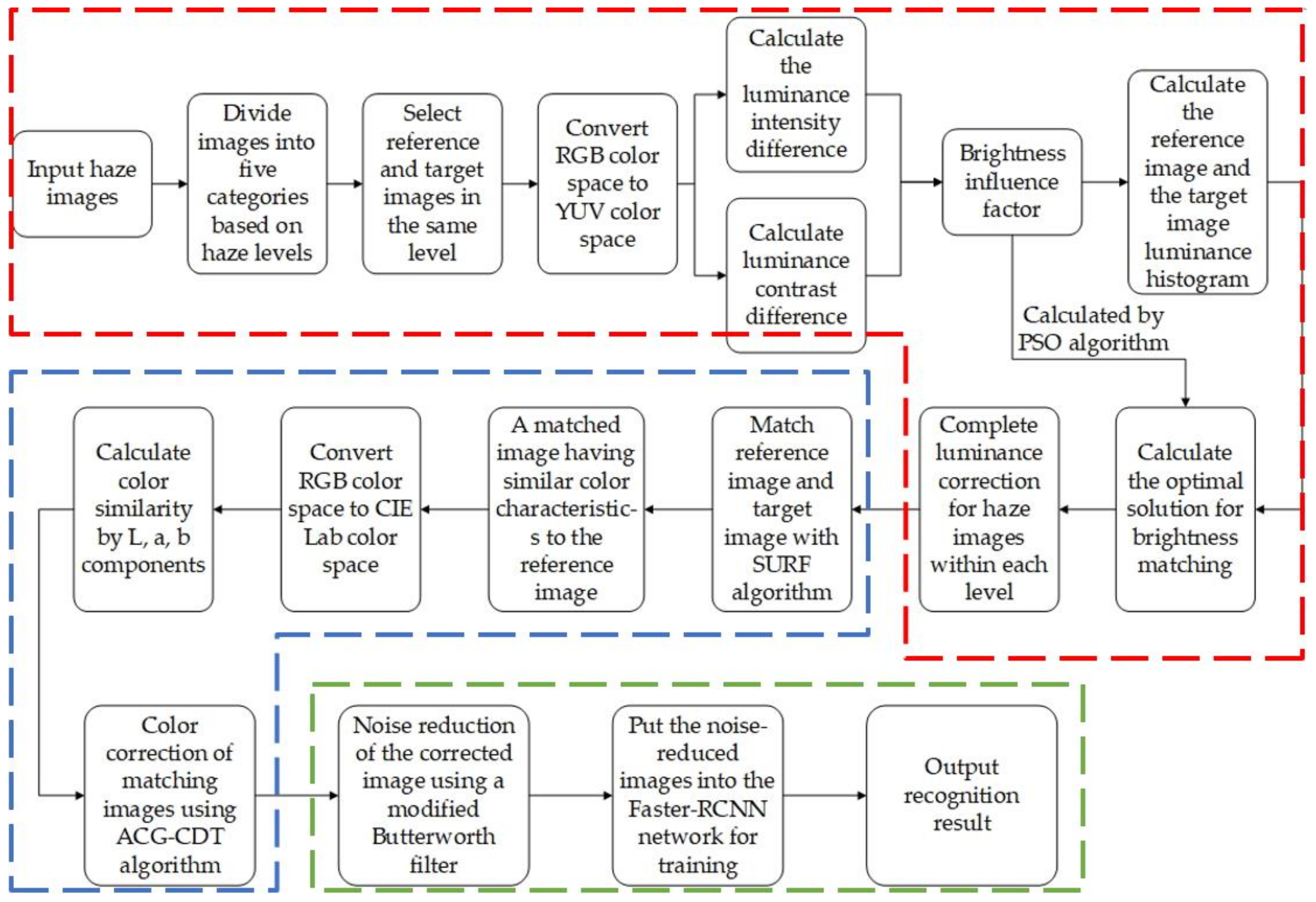
This paper aims to correct the same level of haze images to identify different levels of haze images. First, the difference in brightness of the haze image in the same level need to be corrected. The color similarity of the target image and the reference image is then improved by color correction. Finally, the image is denoised by a filter and the haze level is identified by deep learning. The implementation steps in this paper are shown in Figure 1.

2. Theories

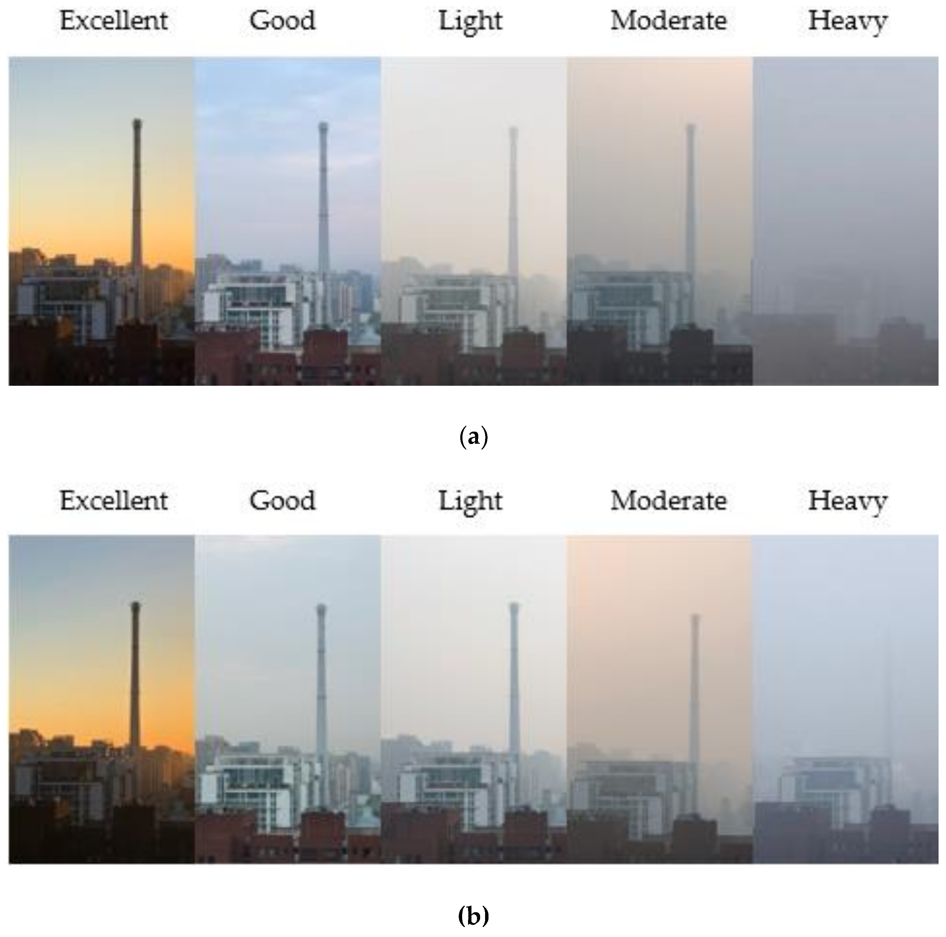
In order to realize the target of haze level recognition based on the haze image processing, this section focuses on the haze image recognition algorithm based on brightness optimization feedback and color correction. In this paper, the images are divided into: excellent, good, light, moderate, and heavy according to the smog level, and an image with appropriate brightness and color is selected from each level as a reference image. The five-level reference image and the target image as an example in each level are shown in Figure 2.
Figure 2a is the group of reference images, Figure 2b is the group of target images. The haze levels from left to right in each group are excellent, good, light, moderate, and heavy.
According to the research purpose, the algorithm of this paper can be divided into the following three stages.
The first stage is to calculate the difference in brightness between the reference image and the target image in each level. Then calculating a parameter α according to the brightness difference between the brightness of the factor; using particle swarm optimization (PSO) algorithm [17] to find the parameter α, which can satisfy the reference luminance image and the target image histogram matching.
The second stage is to use the SURF algorithm to match the corrected target image with the reference image. The matched image has similar structure and color characteristics as the reference image. Then convert the matched image and reference image from RGB color space to CIE Lab color space, and calculating the color similarity of the matched image and the reference image according to the L, a, b color components. Finally, the automated color grading using color distribution transfer (ACG-CDT) algorithm is used to achieve color correction to match the image and the reference image [17].
In the third stage, the improved Butterworth filter is used for the noise characteristics of the corrected image, and the noise-reduced image is trained using the Faster R-CNN network and the recognition result is obtained [18]. The technical route of this paper is shown in Figure 3.

2.1. Brightness Correction Based on PSO Algorithm for Optimal Solution

The reference image and the target image in each level may differ in brightness depending on conditions such as illumination. In this section, by calculating the brightness influence factor of the haze image, the luminance histogram of the reference image and the target image is drawn, and the PSO algorithm is used to solve the optimal parameter α to achieve the brightness histogram matching between the reference image and the target image.

2.1.1. Image Brightness Influence Factor

Since the haze image itself has low brightness and distortion properties, in order to accurately represent the difference in brightness of the haze image, this paper studies the two factors of intensity and contrast in image brightness [19]. First, the input haze image is converted from RGB color space to YUV color space, with Y component as the basis of brightness analysis, and Y component can be expressed as [20]
Y=0.299R+0.587G+0.114B,
where R, G, B are the components of the image in the RGB color space. After obtaining the Y component of the image, calculate the average luminance value of the image which bases on each point (x, y) [21]
μ ( x , y ) = e x p ( 1 n x , y l n ( δ + L u ( x , y ) ) ,
where δ is a small positive number used to prevent the logarithmic calculation from tending to a negative infinity. Lu(x, y) is the luminance value of each pixel on the Y component. After the actual calculation of the average brightness of the haze image, the value of δ in this paper is 0.0001. The average brightness from level excellent to heavy is about 144.2, 151.6, 168.8, 163.4, and 154.8, respectively.
The luminance mean of the reference image and the target image on the Y component can be expressed as μa(x, y), μb(x, y). According to this, the similarity between the brightness of the reference image and the target image can be calculated
l s ( x , y ) = e x p ( | μ a ( x , y ) μ b ( x , y ) θ | ) ,
where θ = 255 represents the dynamic range of variation of the pixel value. The difference in intensity between the two images can be expressed by the trend of the ls value. When ls approaches 0, the difference in intensity between the brightness of the reference image a and the target image b is smaller; when ls approaches 1, the difference in intensity between the reference image a and the target image b is greater.
In addition, it is necessary to calculate the contrast of the image based on the standard deviation between the reference image and the target image. Taking the reference image, the standard deviation equation is
σ a ( x , y ) = 1 M N x = 1 M y = 1 N ( F ( x , y ) μ ( x , y ) ) 2 ,
where F(x, y) is the gray value at the point (x, y) of the input image a, M, N is the height and width of the pixel of the reference image a. The covariance of the brightness of the reference image a and the target image b is σab(x, y). The logarithmic function is used to obtain the similarity in contrast between the two haze images
l c ( x , y ) = l n α ( 1 + σ a b ( x , y ) σ a ( x , y ) ) ,
where α is in the range of (0, 1). Finally, the similarity between intensity and contrast is coupled to calculate the haze image brightness influence factor
l ( x , y ) = l s ( x , y ) · l c ( x , y ) ,

2.1.2. PSO Algorithm for Calculating the Optimal Solution of Histogram Matching

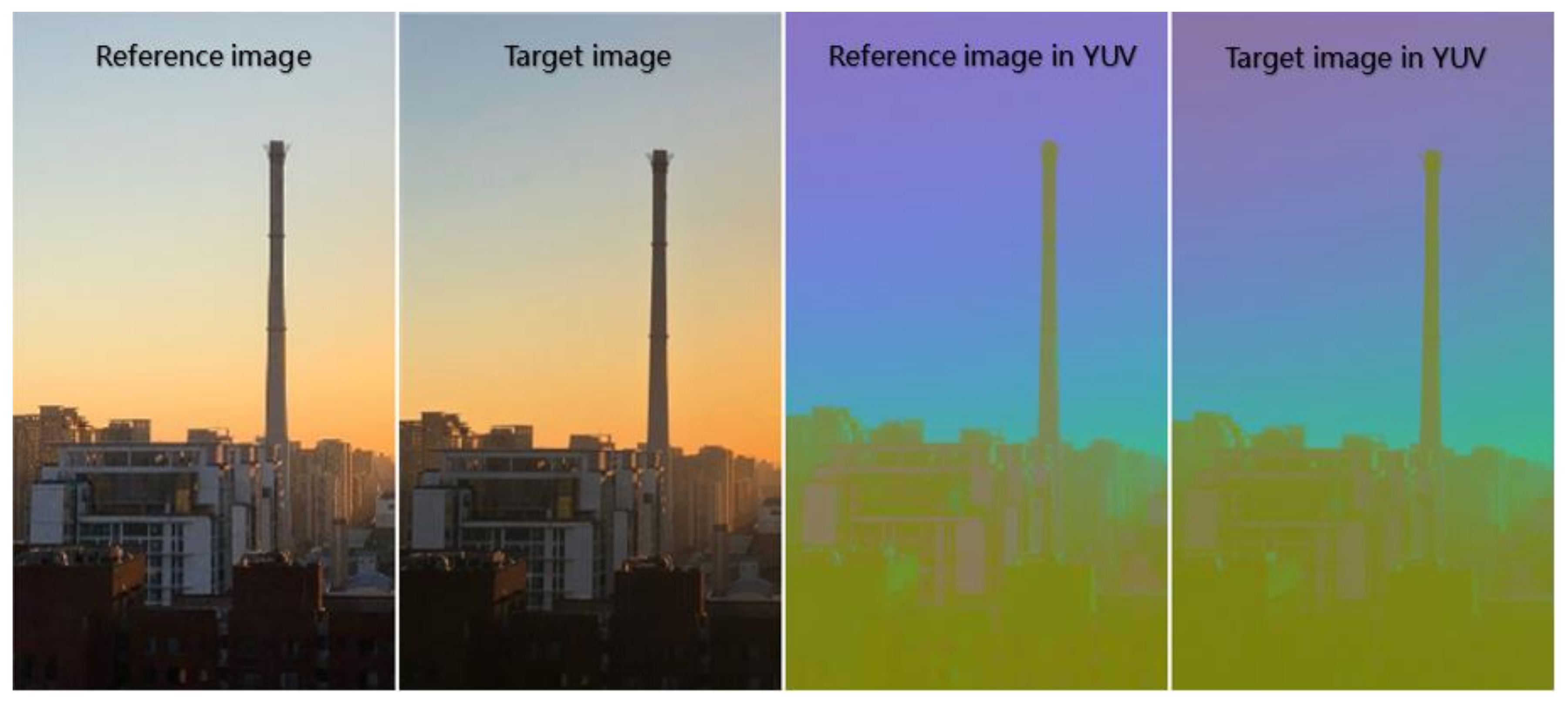
Based on the relevant theories and equations in 2.1, this part calculates the standard image at each level based on the average brightness, and uses the reference image to calculate the brightness difference with the target image and correct it to obtain a corrected haze image. In order to make the target image approximately the same as the brightness of the reference image, it is necessary to find the optimal solution α. Therefore, this paper adopts the PSO algorithm to find the optimal solution α [17]. The PSO algorithm is a global random search algorithm. The PSO algorithm first initializes a certain number of random particles (random solutions) and then finds the optimal solution through iteration. In each iteration, each particle updates itself by tracking its own optimal solution and the optimal solution currently found by the entire particle swarm. The optimal solution α in this paper needs to be calculated by iteration. Furthermore, the average brightness of the output image is similarly corrected by the reference image using the PSO algorithm in the reference [6]. The YUV spatial image is obtained according to the Equation (1). Take the reference image and the target image with the level of excellent as an example, as shown in Figure 4.
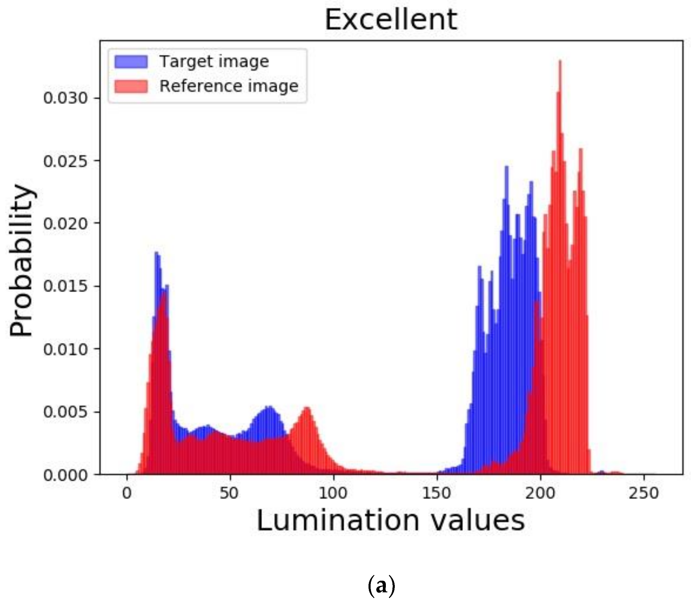
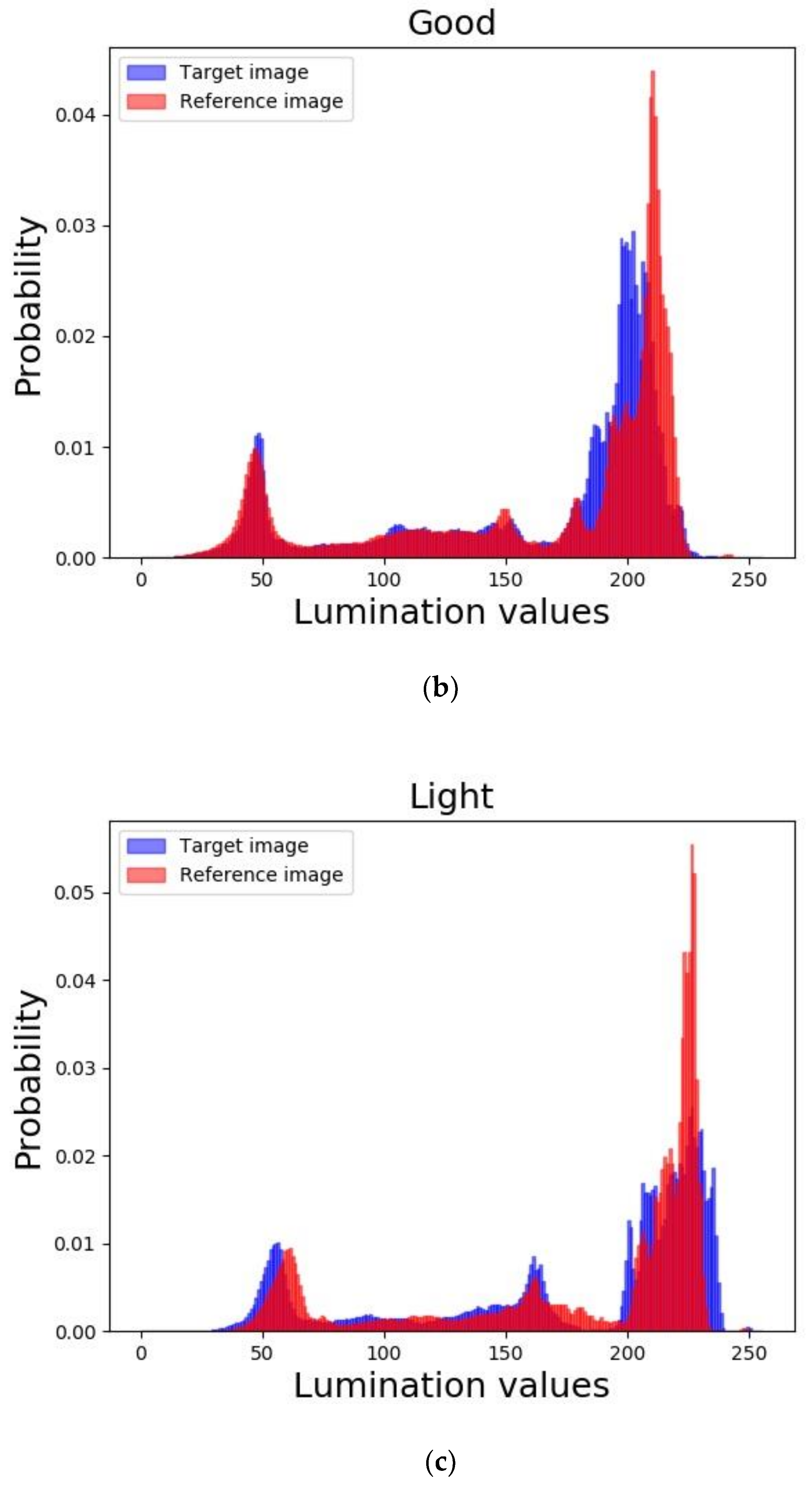
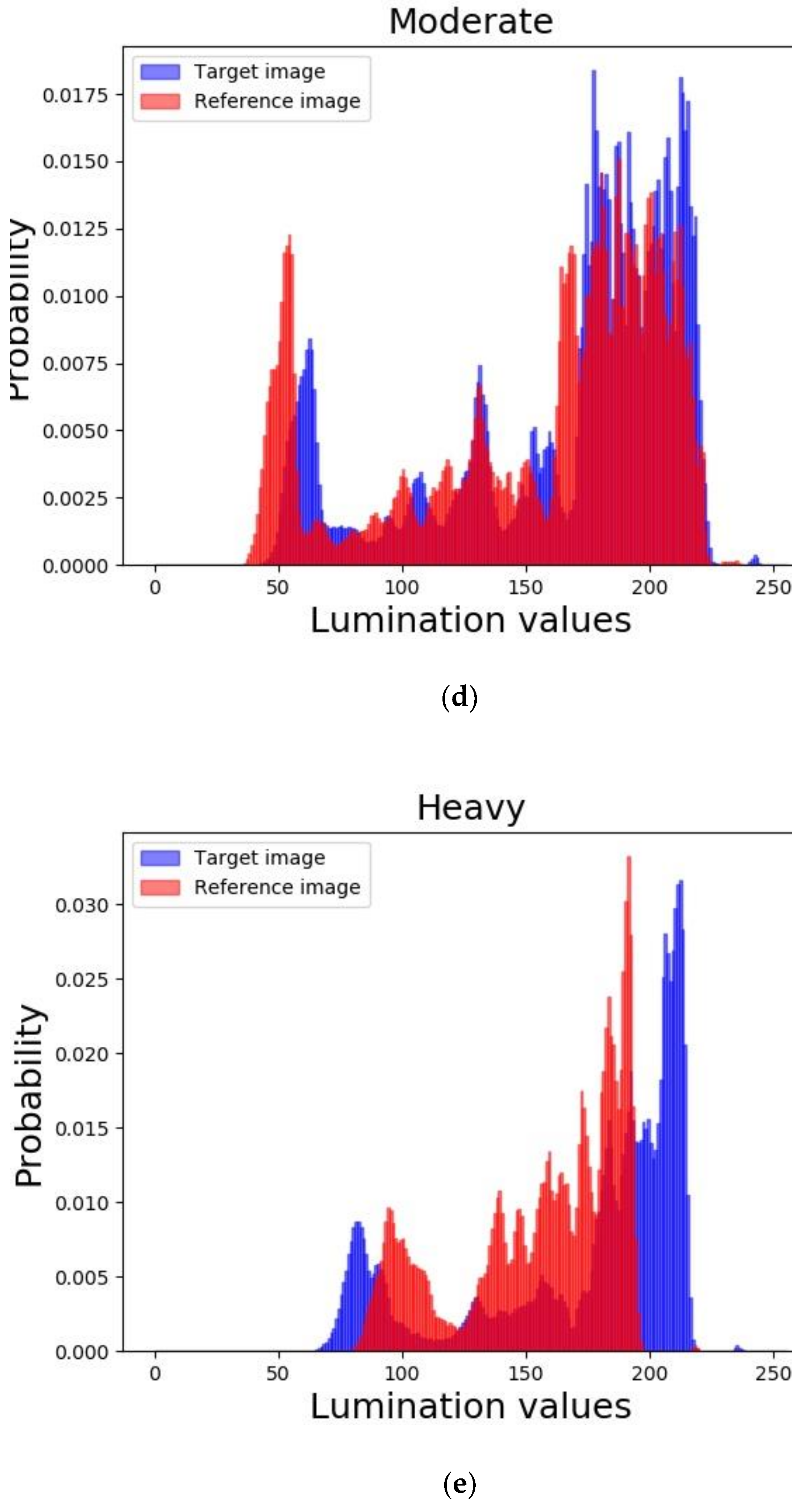
As can be seen from Figure 4, the reference image and the target image are different in the RGB color space and the YUV color space. In order to display the brightness difference between the two images more intuitively and accurately, the luminance histograms of the reference image and the target image on the Y component are respectively calculated, as shown in Figure 5.
As can be seen from Figure 5, the target image in the five levels and the reference image show a significant difference in the luminance histogram. In order to resolve this difference, the luminance of the target image is corrected to the luminance of the reference image according to the Equation (5), and its correction function is
g a ( x , y ) l ( x , y ) · g b ( x + · x , y + · y ) ,
where g a ( x ,   y ) is the luminance value of the reference image at the (x, y) position,   g b ( x ,   y ) is the luminance value of the target image at the (x, y) position, Δ x is the distance difference between the reference image and the target image on the x-axis, Δ y is the distance difference between the reference image and the target image on the y-axis. The luminance of the target image can be corrected to the luminance of the reference image by the Equation (7). However, before the brightness correction is performed, considering the problem that the single haze image itself is unevenly illuminated, the histogram equalization [22] is first performed on the reference image and the target image, respectively. The luminance histogram of the image on the Y component can be regarded as the gray level of the image itself, so the image gray probability is
p r ( r k ) = n k M N , k = 0 , 1 , 2 , , ε 1 ,
where MN is the total number of pixels, k is the k-th brightness value, n k is the number of pixels whose gradation is r k , and ε is the number of gray levels in the image, and the value range is [0, 255]. The cumulative probability of grayscale of an image is
C D F ( r k ) = i = 0 k n i M N ,
From Equation (8) and Equation (9), the result of each pixel equalization can be obtained
D ( r k ) = ε · C D F ( r k ) ,
The equalized reference image and the target image are combined with the target image (7) to solve the optimal value of α in Equation (5). The solution process of the optimal solution is
arg m i n x = 0 M 1 y = 0 N 1 | g a ( x , y ) l ( x , y ) · g b ( x + · x , y + · y ) | ,
where α ϵ R . Converting the Equation (11) to the luminance histogram calculation can be expressed as
Z ( i ) = arg m i n i = 0 255 | D a ( i ) D b ( i ) | ,
where D a ( i ) is the luminance value of the reference image, and D b ( i ) is the target image luminance value multiplied by the brightness influence factor. In this paper, the PSO algorithm is used to solve the α optimal value [23]. Let N particles form a population, where the position of the i-th particle is denoted as P, and bring it into Z ( i ) to obtain the fitness value, and obtain the optimal value of α according to the size of the fitness value. The initial position of the particles in this paper is set according to the range of values of α and can be regarded as random sampling between (0, 1).
The best position of the individual particles is recorded as p b e s t i , the best position of all particles in the whole group is recorded as g b e s t i , and the speed of particle i is recorded as V i t . Therefore, the velocity vector iteration formula of a particle can be expressed as
V i t + 1 = ω · V i t + c 1 · r 1 · ( p b e s t i P i t ) + c 2 · r 2 · ( g b e s t i P i t ) ,
where c 1 and c 2 are learning factors. r 1 and r 2 are random numbers with a value range of [0, 1]. In addition, the inertia weight ω is as shown in Equation (14)
ω = ω m a x ( ω m a x ω m i n ) · t t m a x ,
where t is the current number of iterations and t m a x is the maximum number of iterations., and its value range is set to [ ω m i n , ω m a x ] . Based on the above, the update equation of speed V i t + 1 and position P i t + 1 is
P i t + 1 = P i t + V i t + 1 ,
Finally, the solution process of the α optimal value is implemented in Algorithm 1.
Algorithm 1: choosing the best α using PSO
    Input: Reference image D a ( i ) and target image D b ( i , l )
    Create N particles { P 1 , P 2 , , P N } , where P i R representing an α;
    for each particle i   =   1 : N do
      Initialize the position of each particle P i 1 and its corresponding velocity V i 1 ;
    end for
    for t   =   1 : t m a x do
      for each particle
        Calculate the objective function Z i t using equation (12);
          if Z i t < Z ( p b e s t i )
             p b e s t i = P i t ;
          end if
          if Z i t < Z ( g b e s t i )
             g b e s t i = P i t ;
          end if
         end for
       for each particle i   =   1 : N do
         update the velocity V i t + 1 using equation (13)
         update the velocity P i t + 1 using equation (15)
       end for
     end for
     Output: the optimal α *

2.2. Color Correction Algorithm Based on Feature Matching

Due to factors such as shooting angle and image acquisition time, each haze image still has chromatic aberration after brightness correction. Automated color grading using color distribution transfer (ACG-CDT) can be nonlinearly corrected by establishing a color map between images [17], but the effects of image position differences cannot be avoided. To this end, this paper proposes a color correction algorithm based on feature matching to improve the color difference between the reference image and the target image. This algorithm can be divided into the SURF algorithm to match the target image with the reference image, and the ACG-CDT algorithm to calculate the color correction result. The color correction result can be judged by calculating the color similarity of the images before and after the matching.

2.2.1. Color Similarity

The color similarity is calculated based on the color difference between the images, and the purpose is to accurately represent the difference in color between the two images. Considering that the color components of the RGB color space are not independent of each other, the color similarity is calculated for the image a and the image b using the CIE Lab color space which is more in conformity with the parallax. Since the haze images acquired by the camera is an RGB color space, it is necessary to convert RGB to CIE Lab [24]. From this, the color difference between the haze images a and b in the Lab color space can be calculated
Δ E = Δ L 2 + Δ a 2 + Δ b 2 ,
where ΔE represents the color difference of the target image a and the matching image b. ΔLab represents the difference between the two pictures on different components, respectively. The color similarity of the two can be calculated by the color difference between the reference image a and the matching image b [25]
S ( p a , p b ) = { e k Δ E Δ E < γ 0 Δ Ε γ ,
where γ is the maximum color difference between each pair of pixels of the two figures, and k is the weight of color difference, which is set to 0.000001 in this paper. Two identical pictures have a color similarity of 1, and two completely different pictures have a color similarity of zero. The color similarity between the reference image and the matching image in the five levels is S ( p a , p b ) .

2.2.2. Image Matching and Color Correction

This paper uses the SURF algorithm to match the target image with the reference image. Since the image which matches pixel obtained from the reference image, the reference image which has similar color characteristics. In this paper, the correction result is obtained by using the feature matching region of the reference image and the target image. Then, the feature point M1 of the reference image is compared with the M2 feature points of the registration image, and the Euclidean distance is calculated and sorted. In this paper, the feature subset registration method is used to improve the computational efficiency.
  • Construct a scale space of the reference image and the registration image. Calculate the number of reference image scale spaces to form N feature sets; calculate the number of registration image scale spaces, form M feature sets, and arrange the two image feature sets according to their scale.
  • The registration image feature set is unchanged, and the feature set of the reference image is in one-to-one correspondence with the feature set of the registration image. Calculate the matching logarithm of the corresponding feature point.
  • The registration image feature set is unchanged, the feature set of the reference image is arranged in reverse order, and the matching logarithm of the corresponding feature point is recalculated.
  • Compare the feature matching logarithm of two times and the maximum value of the two matchings as the feature point matching relationship. This relationship is used as the image registration relationship to calculate the affine matrix and achieve registration.
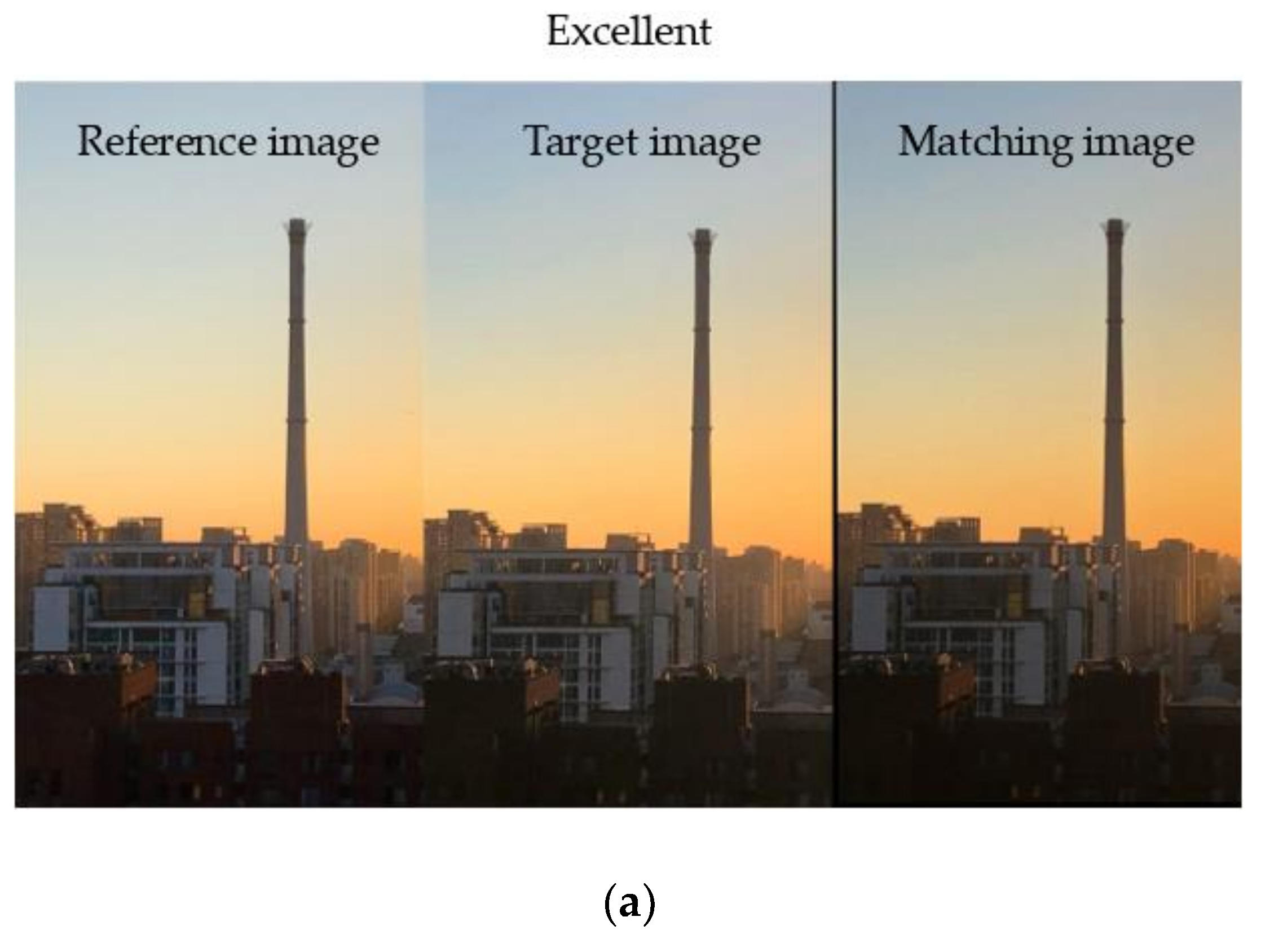
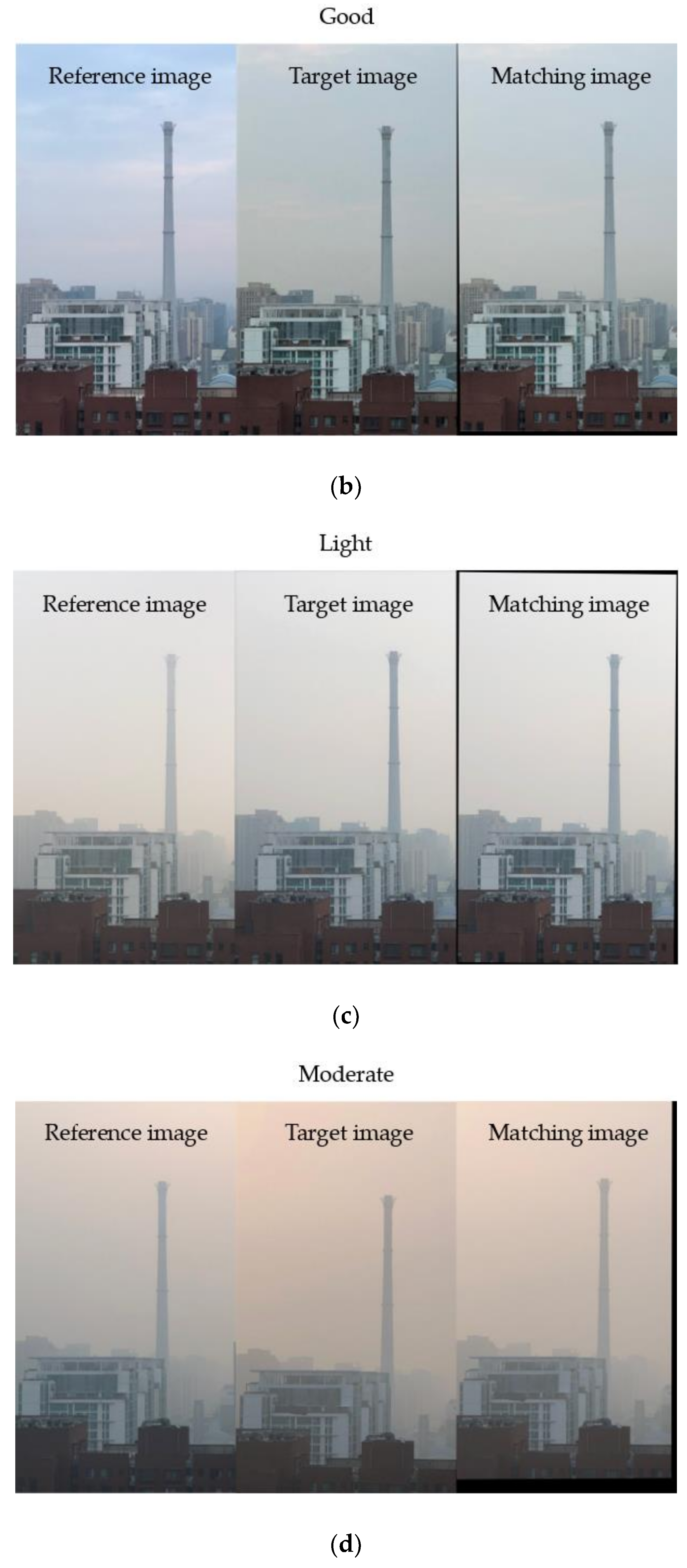
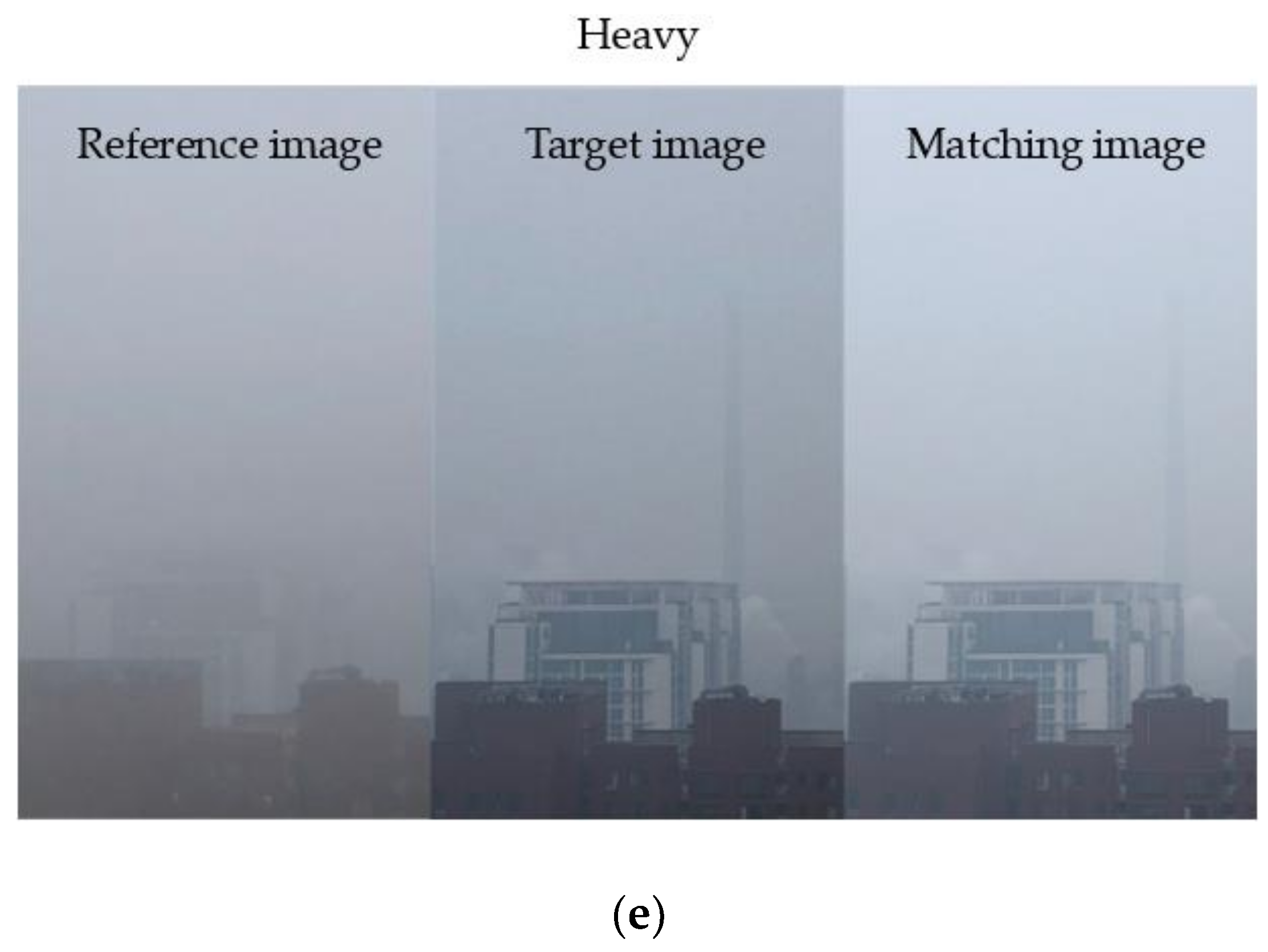
The matching image produced by the above steps has a similar structure to the reference image. Furthermore, the pixels of the matching image are from the reference image, and thus their color characteristics are also consistent with the reference image. The reference image and matching image under the same haze levels are shown in Figure 6.
In Figure 6, each group of pictures from left to right contains a reference image, a target image and a matching image. According to Figure 6, the matching image is the same as the target image, and the color is similar to the reference image. Due to the shooting angle, a non-matching area appears between the reference image and the matching image and is displayed in black.
Based on the matching images, the ACG-CDT algorithm is used to correct the matching images [17]. In this paper, the color similarity S ( p a , p b ) between the reference image a and the matching image b is calculated by the equation (16) and the equation (17), and the threshold is set according to the color similarity. Let I m be the matching image, I r is the corrected image after ACG-CDT, and the final correction result I f is
I f ( i , j ) = { I m ( i , j ) S ( p a , p b ) < 0.8 I r ( i , j ) S ( p a , p b ) 0.8 ,
where ( i ,   j ) is the position of the pixel. If S ( p a , p b ) is less than 0.8, the color in the matching image at the ( i ,   j ) position is selected. Otherwise, the image color is corrected using the ACG-CDT algorithm.

2.3. Improved Butterworth Filter

Although the luminance difference and chromatic aberration of the corrected haze image are improved, the correction does not eliminate the noise of the haze image itself. In addition, the characteristics of the image in the haze environment are not obvious, so it is particularly important to use filters to improve the image quality of the haze. This section is based on the Butterworth filter and is improved based on the characteristics of the haze image. The improvement is to eliminate image noise while preserving image edge features. In addition, the peak signal-to-noise ratio (PSNR) is selected as the test standard for filtering results [26].
The image is transformed from the spatial domain to the frequency domain for image enhancement processing [27]. Then the image is returned from the frequency domain to the spatial domain, and the enhanced image can be obtained [28].
Using a two-dimensional discrete Fourier transform for haze images, the formula for the discrete Fourier transform of the haze image f ( x , y ) of size M * N is
F ( u , v ) = 1 M N x = 0 M 1 y = 0 N 1 f ( x , y ) e j 2 π ( u x M + v y N ) ,
among them, x = 0 , 1 , 2 , , M 1 ; y = 0 , 1 , 2 , , N 1 . The variables u and v are frequency variables, the variables x and y are called spatial variables.
In the frequency domain, f ( x , y ) is the input haze image, F ( u , v ) is the Fourier transform of the haze image, and G ( u , v ) is the haze image after the transformation. Based on the frequency domain, the output image can be calculated as
G ( u , v ) = F ( u , v ) 1 + F ( u , v ) H ( u , v ) ,
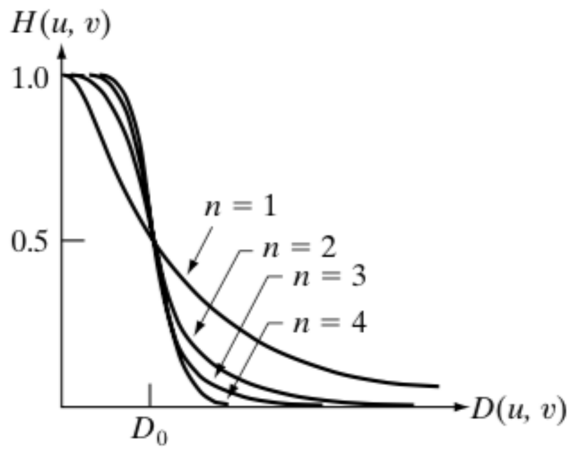
among them, H ( u ,   v ) is the filter function in the frequency domain. Thus, the denoised image can be got by using the inverse Fourier transform. The Butterworth filter has a smooth transition between low and high frequencies, thus avoiding noticeable ringing effect. The traditional Butterworth filter is [22]
H ( u , v ) = 1 1 + [ D ( u , v ) D 0 ] 2 n ,
where D 0 is the cutoff frequency, D ( u , v ) is the distance from the point ( u , v ) to the origin in the Fourier frequency domain. The traditional Butterworth filter function is shown in Figure 7.
According to the above Figure 7, when the value of n is larger, the function is closer to the ideal filter, but the ringing effect is also greater. In combination with the self-characteristics of the haze image, this section selects n = 1 for improvement. Traditional Butterworth filter loses a large amount of high frequency signals during noise reduction, which results in an unclear edge contour of the image. In this paper, high frequency gain R h and low frequency gain R 1 are introduced for this problem. The purpose is to increase the pass of high frequency signal while keeping the low frequency signal as much as possible. The transfer function of the improved Butterworth filter H ( u , v ) is
H ( u , v ) = R l R h 1 + c D ( u , v ) D 0 + R h ,
among them, R h is the high frequency gain, R 1 is the low frequency gain, and c is constant. In this paper, to preserve the low frequency signal, lets R 1 > 1 ; at the same time, lets 0 < R h < 1 to ensure the pass of high frequency signal and R l R h > 0 . In addition, R h can guarantee that the equation is greater than 0 in any case. Equation (22) can enhance the edge detail and contrast of haze images while removing a small amount of high frequency signal noise.

2.4. Haze Image Recognition Based on Faster R-CNN

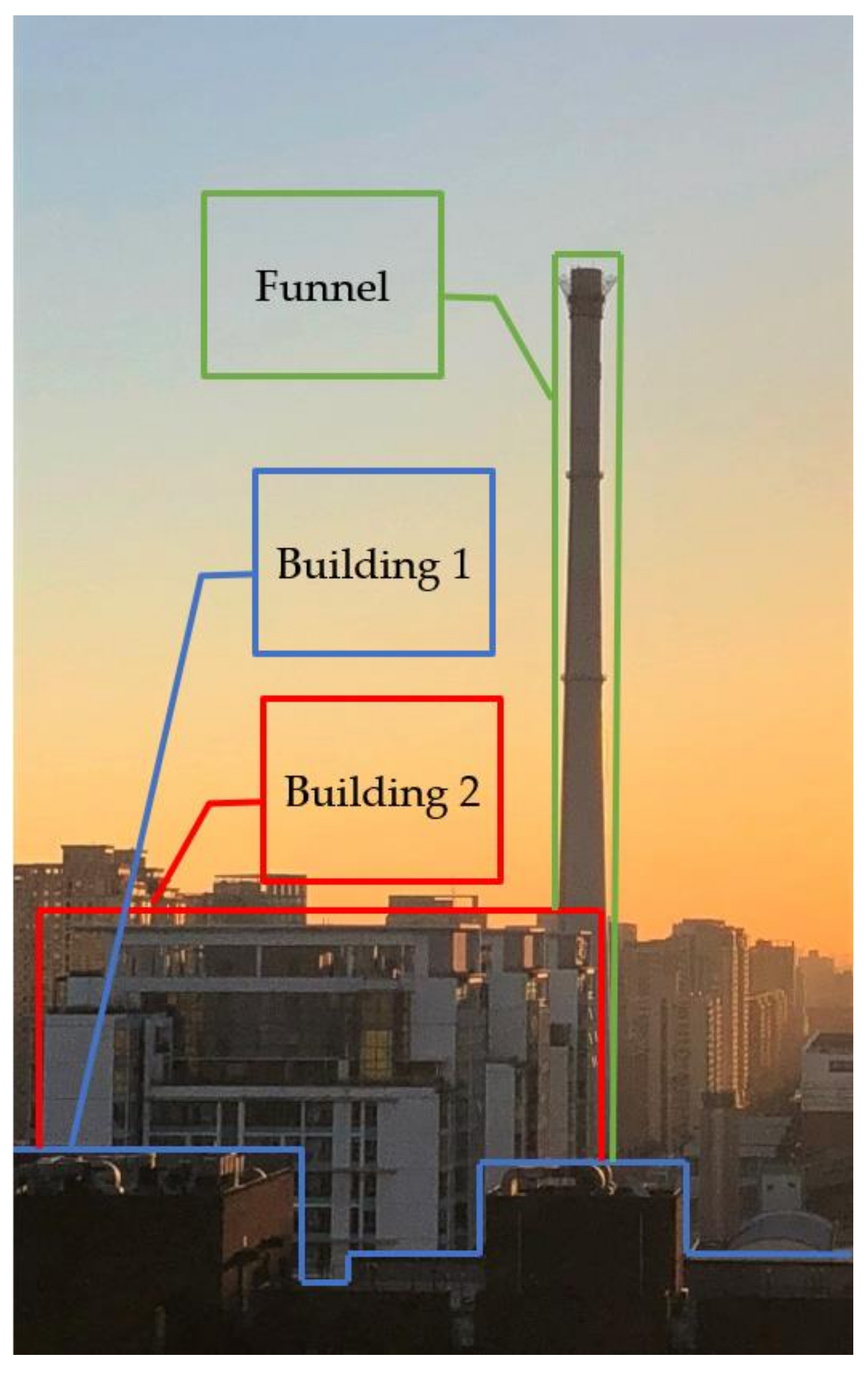
The haze images after correction and noise reduction can meet the requirements for recognition of the haze levels. In this paper, samples of the haze images are classified and marked according to the haze levels, and specific buildings are marked for the haze images in each level. Take the image with the level of excellent as an example, and the result of the marking is shown in Figure 8.
In Figure 8, the darkest building is labeled "Building 1", the light building is labeled "Building 2", and the funnel is labeled “Funnel”. On this basis, this paper uses Faster R-CNN to extract image features and identify them according to the mapping relationship between haze level and calibration objects.
Faster R-CNN is based on Fast R-CNN [29]. Faster R-CNN is mainly composed of three parts:
  • Basic feature extraction network;
  • RPN (region proposal network);
  • Fast R-CNN. The RPN and Fast R-CNN networks share parameters through alternate training.
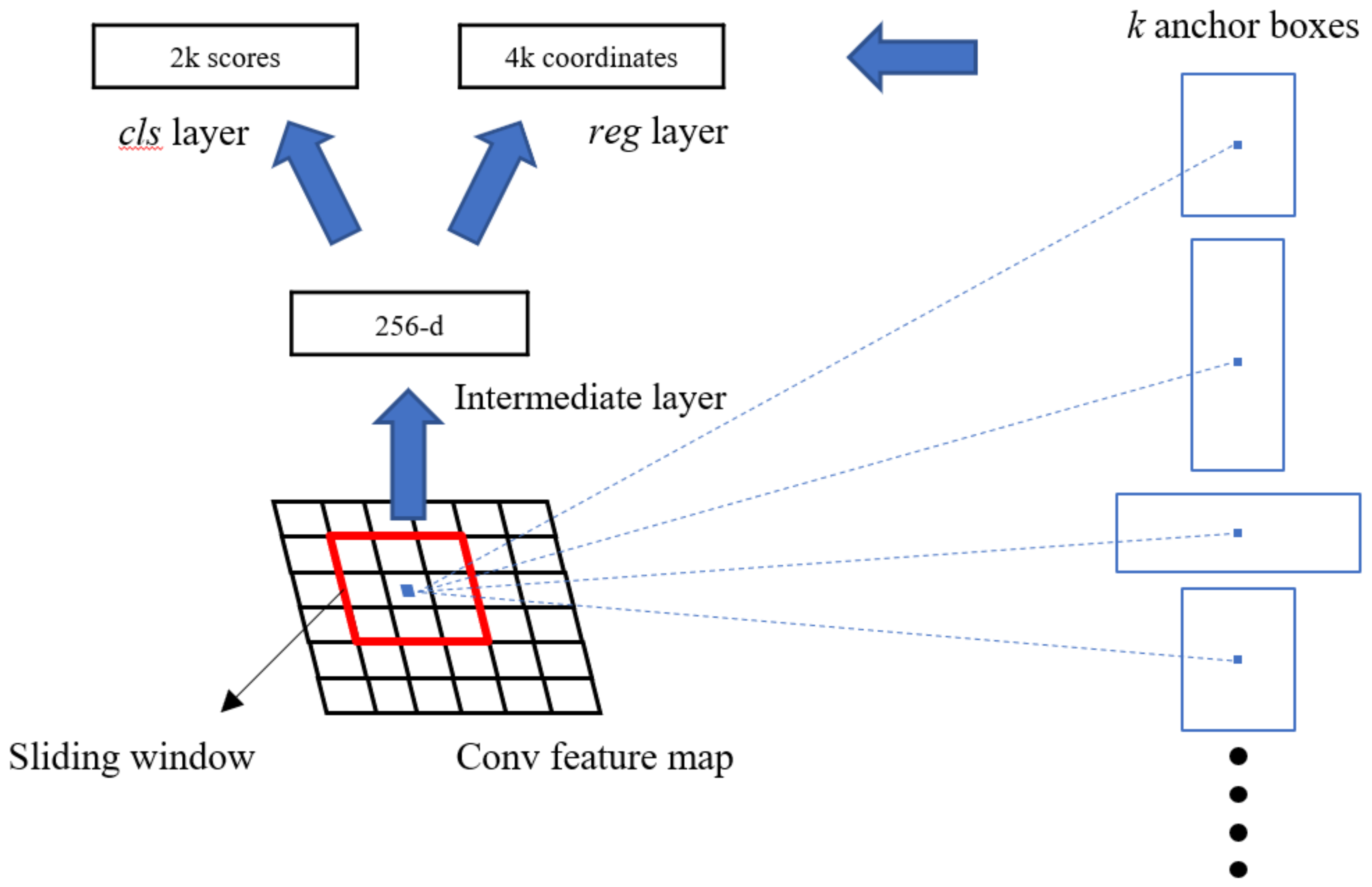
The RPN network structure is shown in Figure 9 below [18]:
The RPN network first uses a CNN model as a feature extractor to extract the feature map of the input image. This paper chooses ResNet as the feature extraction network [30]. Then, using n * n sliding window on the feature map, a low-dimensional feature (256-d) is mapped to each sliding window position. In this paper, n is taken as 3 according to the haze images. These features are fed into two fully connected layers for classification and regression, with each sliding window location sharing two fully connected layers. For each window position, k different sizes or ratios of default bounding boxes are generally set, which means that each position predicts k regions proposals. This article uses three scales and three aspect ratios, yielding k = 9 anchors at each sliding position. For the classification layer, the output size is 2 k , indicating that each candidate region contains an object or a probability value of the background, and the regression layer outputs 4 k coordinate values indicating the positions of the respective candidate regions. Training the loss function of the RPN network which defined in [18] is
L ( { p i } , { t i } ) = 1 N c l s i L c l s ( p i , p i * ) + λ 1 N r e g i p i * L r e g ( t i , t i * ) ,
After RPN network training, this paper uses Fast R-CNN to detect and use Fast R-CNN to train a separate detection network. At this process, RPN and Fast R-CNN do not share features. Then, according to the four-step alternating training method in [18], the RPN and the Fast R-CNN share characteristics, and finally a unified network composed of RPN and Fast RCNN with shared convolutional layer is realized. Through the training of Faster R-CNN, the accuracy of the data samples on the test set is used as the criterion for judging the level of the haze image.
When the image to be tested passes the brightness correction, color correction and noise reduction processing, the recognition result is recorded as 1 when the level corresponding to the image is the same, and 0 when it is not the same. The final accuracy can be expressed as
A C C = T ( Z ,   I f ,   G ) T ( Z ,   I f ,   G ) * 100 % ,
where Z, I f , G are the results of equation (12), equation (18) and equation (20), respectively. T ( Z ,   I f ,   G ) represents the total number of samples that can be used as a test set after processing, and T ( Z ,   I f ,   G ) represents the number of samples identified as 1 by the Faster R-CNN network.

3. Experiments and Comparisons

According to the above, the final research of this paper aims to correct the brightness and color difference between the same level of haze images, and design a filter that can reduce the haze images noise, and finally using the Faster R-CNN network to realize the identification of the level of haze. The experiments in this paper are finally reflected in the accuracy of the test set. Therefore, the experiments can be composed of four parts, including: contrast experiment of brightness correction, contrast experiment of color correction, contrast experiment of filter and contrast experiment of recognition model.

3.1. Image Data Description

In the case of keeping the shooting position relatively consistent, this article photographed 2,100 haze images with different brightness and chromatic aberration. The shooting location is in an open area with buildings, shooting from 7:00 a.m. to 9:00 a.m. Each image is 540 pixels wide and 960 pixels high. At the same time, the images are classified and marked according to the actual air quality at the time of shooting. According to the Air Quality Index (AQI) [31], this article classifies the haze levels into five levels, as shown in Table 1.
In the course of the experiment, this paper selects 10% of the images in the data set as the test set and 90% of the images as the training set. The results of all experiments are shown as the accuracy of haze levels identification. The CPU model used in this experiment is: Intel (R) Core (TM) i5-4460, RAM is 16GB, the graphics card is GTX1080. The implementation of experiment-related algorithms is based on Python 3.5 development.

3.2. Brightness Correction Experiment

According to the study in Section 2.1.1, the average brightness value of the haze images in the five levels is calculated, and the average brightness in each level is as shown in Figure 10.
In Figure 10, the average brightness value of the image with the level of excellent is 144.2, and the fluctuation range is about (142, 146); the average brightness value of the image with the level of good is 151.1, and the fluctuation range is about (149, 153); the average brightness value of the image with the level of light is 168.8, and the fluctuation range is about (167, 171); the average brightness value of the image with the level of moderate is 163.4, and the fluctuation range is about (162, 165); the average brightness value of the image with the level of heavy is 154.8, and the fluctuation range is about (153, 156).
As can be seen from Figure 10, the difference in the average brightness values between the levels is remarkable. However, the average brightness values of the images in each level vary greatly, and the outliers in each level appear similar to the normal values of other levels. It is therefore necessary to correct the difference in brightness between images in each level.
Therefore, this paper corrects the difference in brightness between images by the PSO algorithm. According to the study in Section 2.1.2, the particle initialization of the image in each level is shown in Table 2.
The parameters used in the PSO algorithm are based on the literature [23] as shown in Table 3.
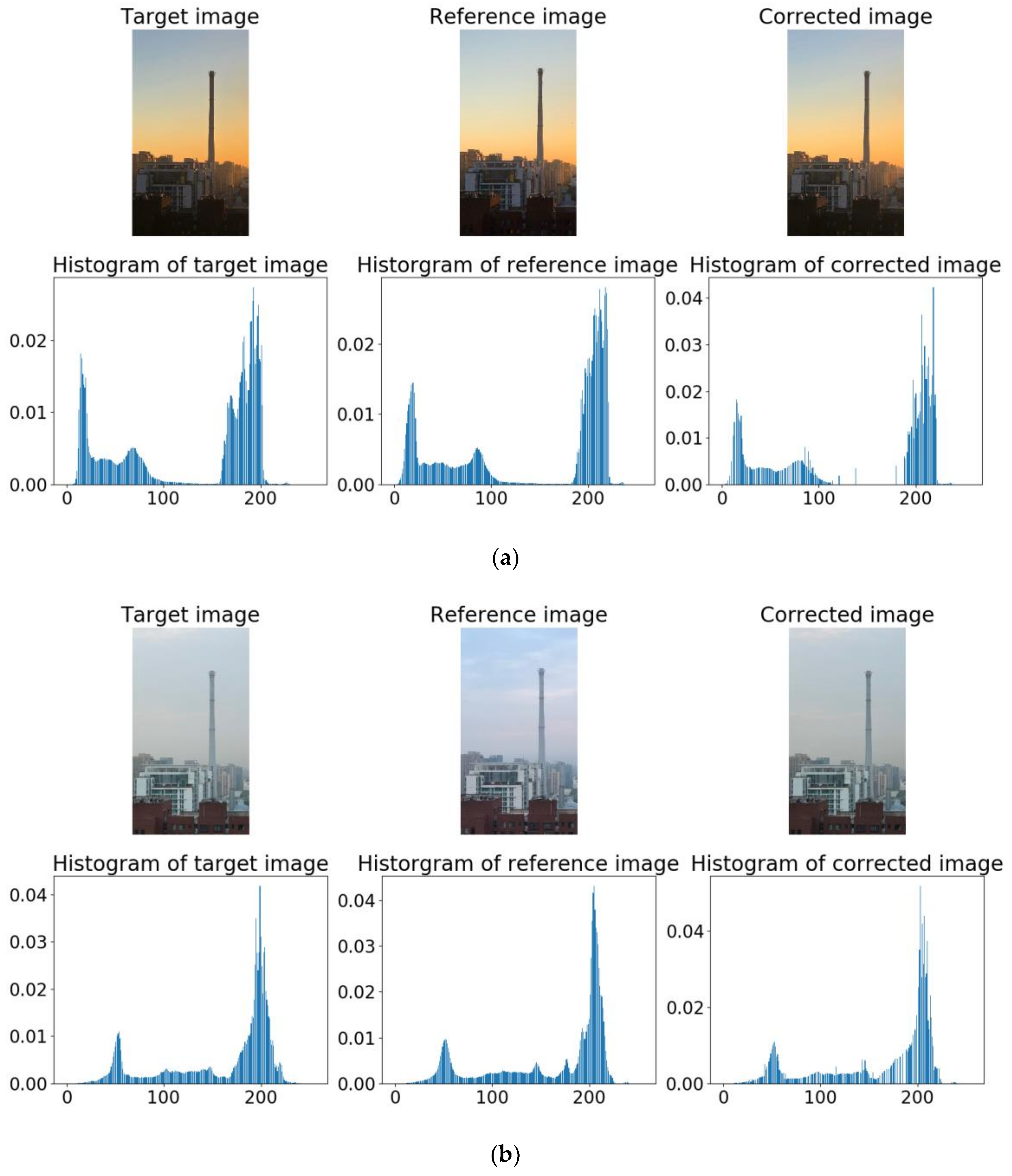
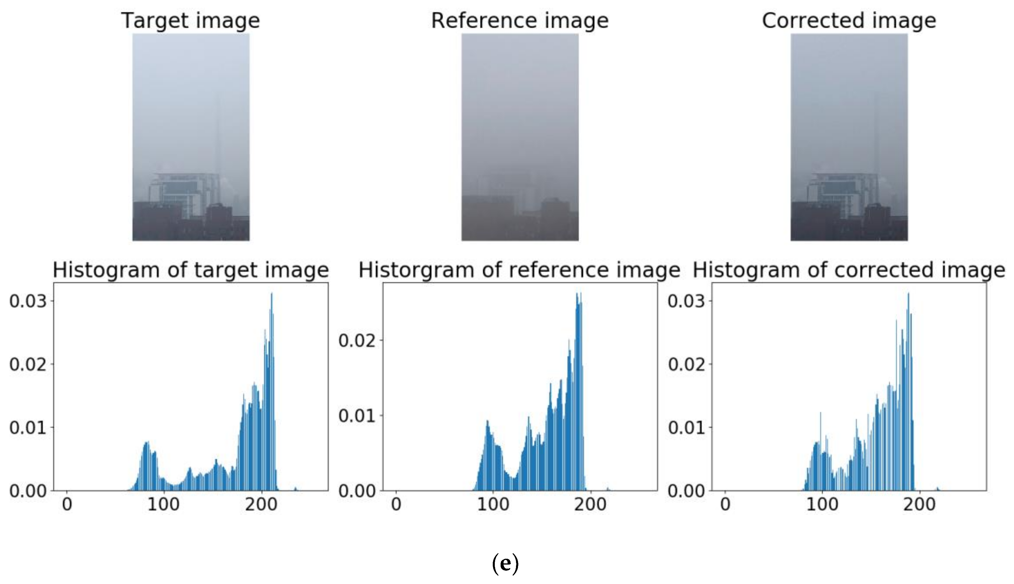
The final brightness corrected image that can be obtained by the above steps, the corrected haze image and its luminance histogram are as shown in Figure 11.
From Figure 11, the subjectively corrected target image is closer to the reference image in terms of brightness, and the luminance histogram of the objectively corrected target image is closer to the luminance histogram of the reference image.
In order to further show the effects before and after the correction, the similarity between the reference image and the luminance histogram of the target image, the similarity between the reference image and the luminance histogram of the corrected image, and the degree of improvement of the latter compared with the former are calculated respectively. The specific results are shown in the table below.
According to Table 4, the luminance histogram of the corrected image is more similar to the reference image. Due to the interference of the color difference between the partial images, the luminance histogram of the corrected image cannot be completely matched to the reference image.
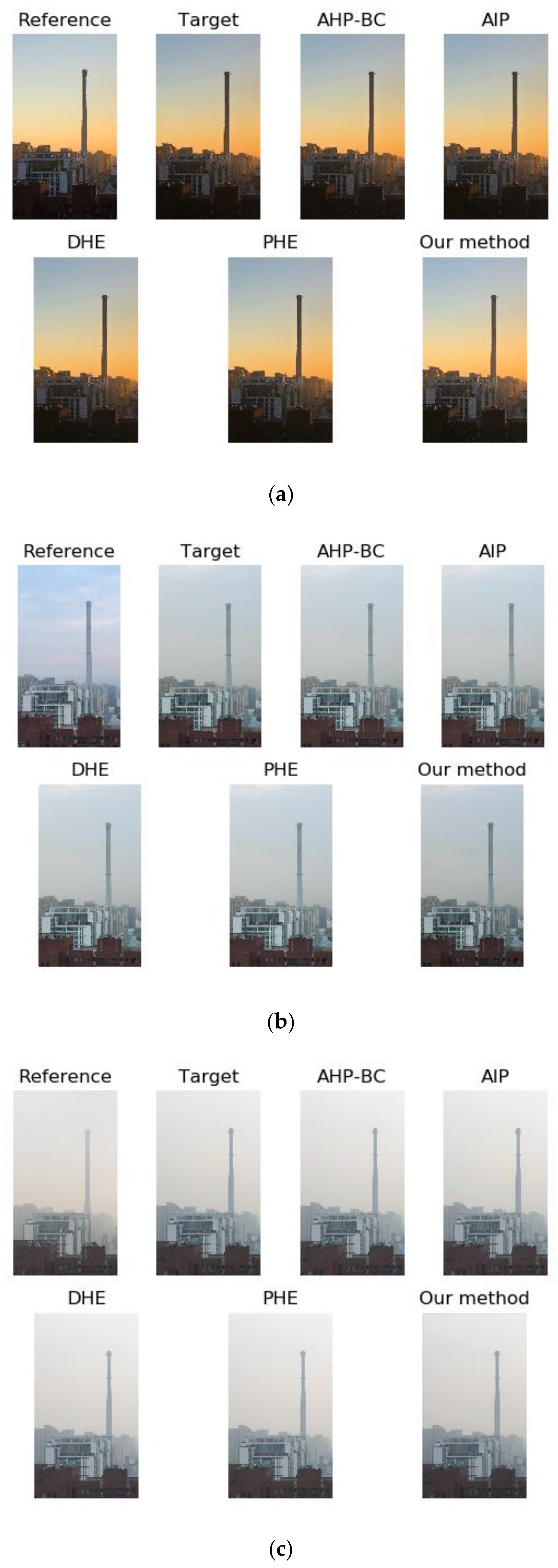
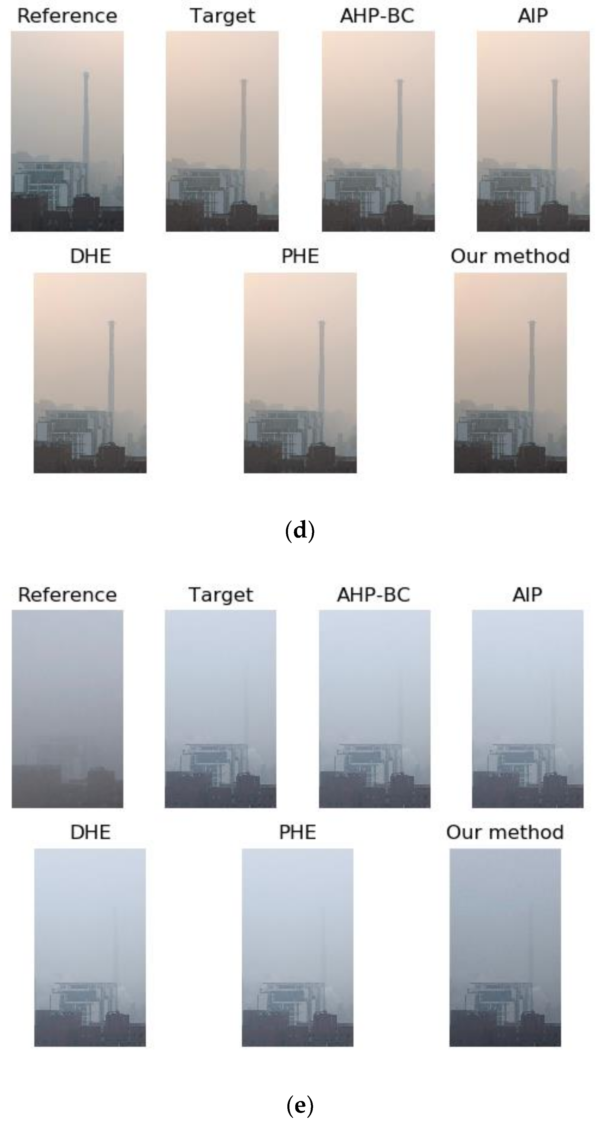
In order to verify the effectiveness of the brightness correction algorithm, this paper chooses (AHP-BC) [6], (AIP) [7], DHE [8], PHE [9] to compare with the brightness correction algorithm in this paper. Their comparison results are shown in Figure 12.
It can be seen from Figure 12 that when the level is excellent, the brightness difference between the images corrected by different methods is not large and close to the brightness of the reference image; however, as the air quality decreases, the correction results of different methods are more obvious. The difference, for example, the correction results of AHP-BC, AIP, DHE and PHE in Figure 12c are significantly different from the reference image. In addition, according to the comparison images of each group, AHP-BC, AIP, DHE, and PHE have similar results of correction. The brightness correction method in this paper is obviously improved.
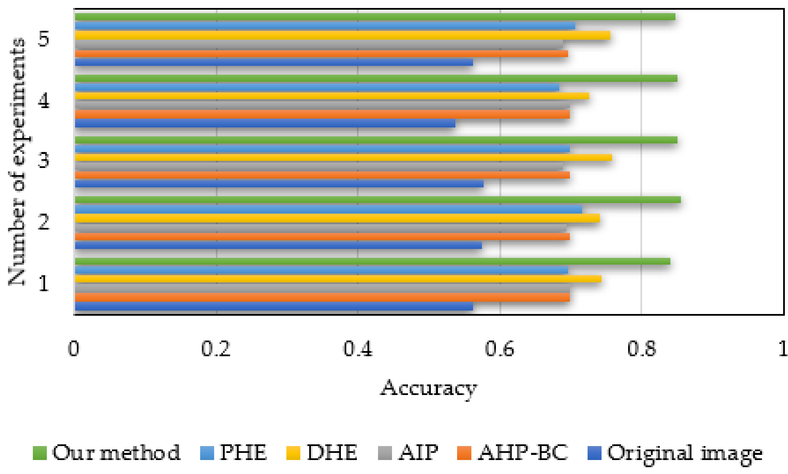
In order to more objectively compare the effects of several brightness correction algorithms, this paper performs haze images recognition based on only changing the brightness correction algorithm. The experiment on the test set was repeated five times, and the accuracy of each time is shown in Figure 13.
According to the five repeated experiments, it can be concluded that the brightness correction method of the brightness correction method has an accuracy of about 85% over five repeats; the unprocessed original image has the worst accuracy of only about 55%; after other brightness the accuracy of the correction algorithm is about 70%. In addition, through the horizontal comparison of the five experiments, the accuracy of the unprocessed original image fluctuated greatly, and the fluctuation of the accuracy of the image after the brightness correction was more stable. In summary, the result of the brightness correction algorithm in this paper is better in the comparison experiments.

3.3. Color Correction Experiment

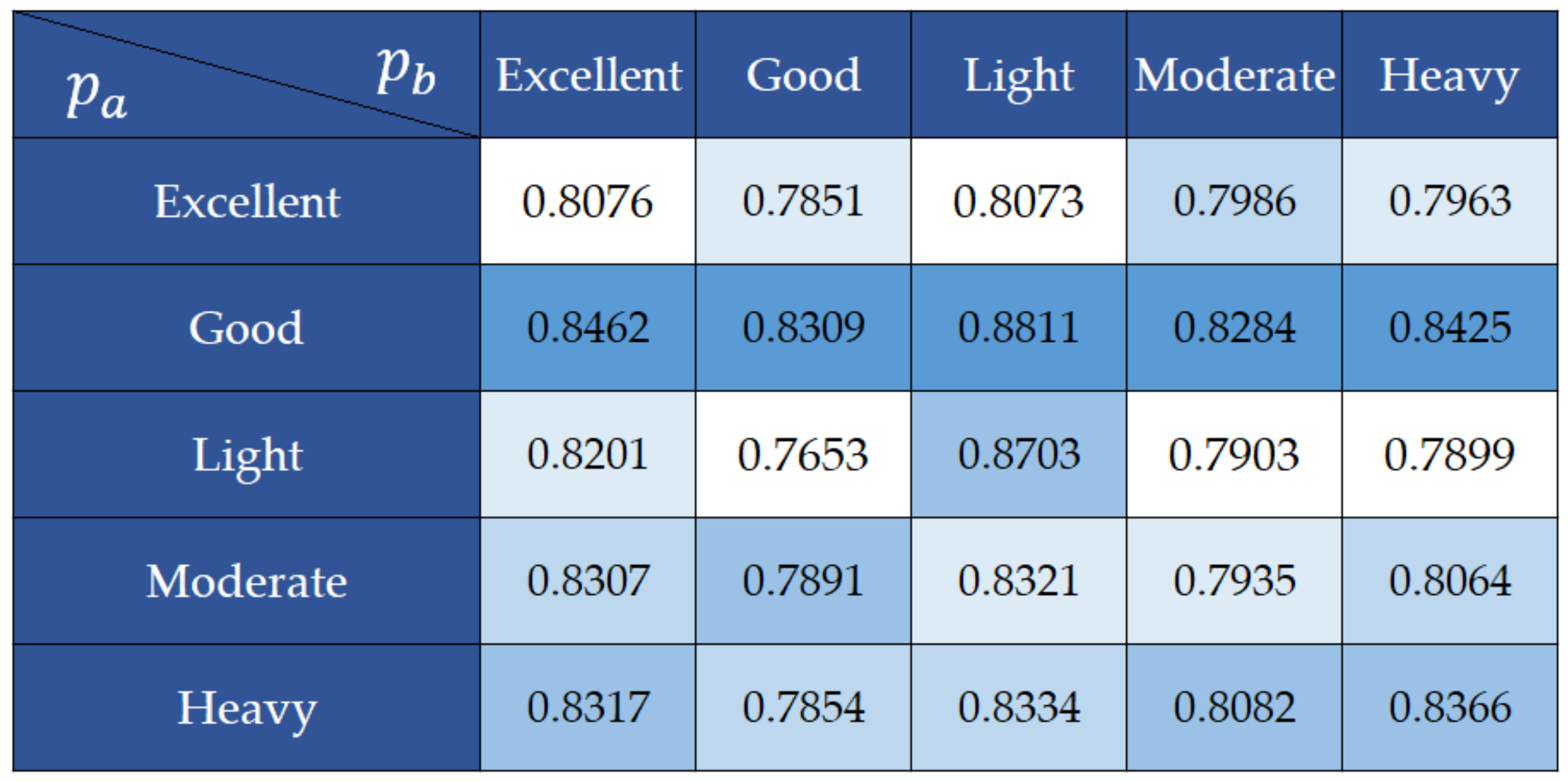
According to the study in Section 2.2.1, the color similarity between images is first calculated before color correction. The calculation results are shown in Figure 14.
In Figure 14, p a represents a target image, and p b represents a reference image, which includes five levels of excellent, good, light, moderate, and heavy, respectively. The numerical values in Figure 14 represent the color similarity between the target image and the reference image. As can be seen from Figure 14, most of the reference image and the target image under the same level do not have the greatest similarity. Taking the reference image at the level of excellent as an example, the color similarity between the images at the same level of excellent is only 0.8076; and the color similarity between the reference image at the level of excellent and the target image at the level of good is 0.8462. The difference between the two is 4.78%.
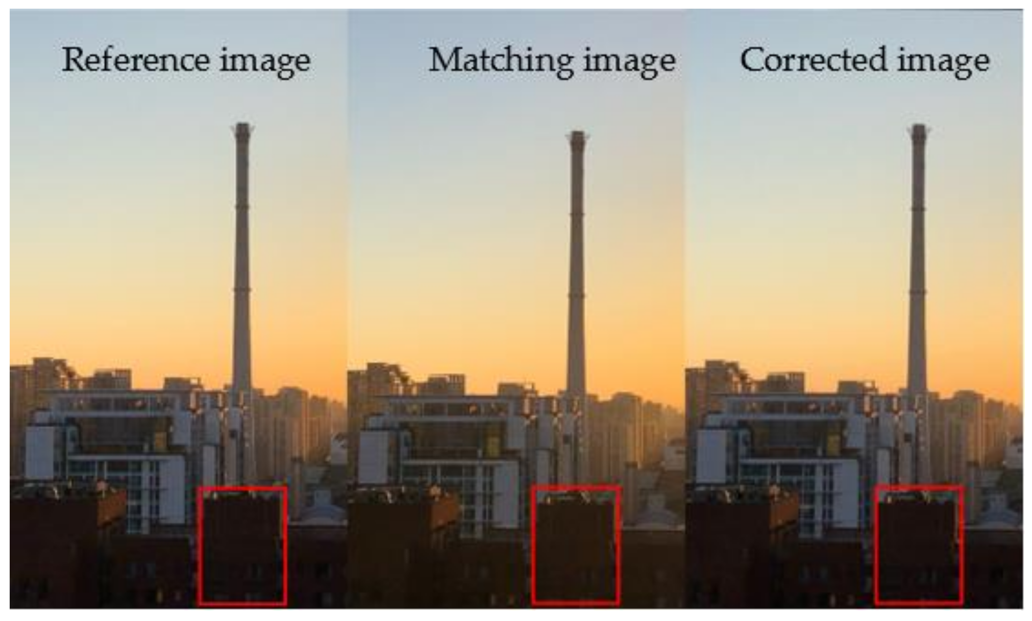
The feature-matched image and the reference image are corrected by the study of Section 2.2.2. Taking the image with the level of excellent as an example, the correction result is shown in Figure 15.
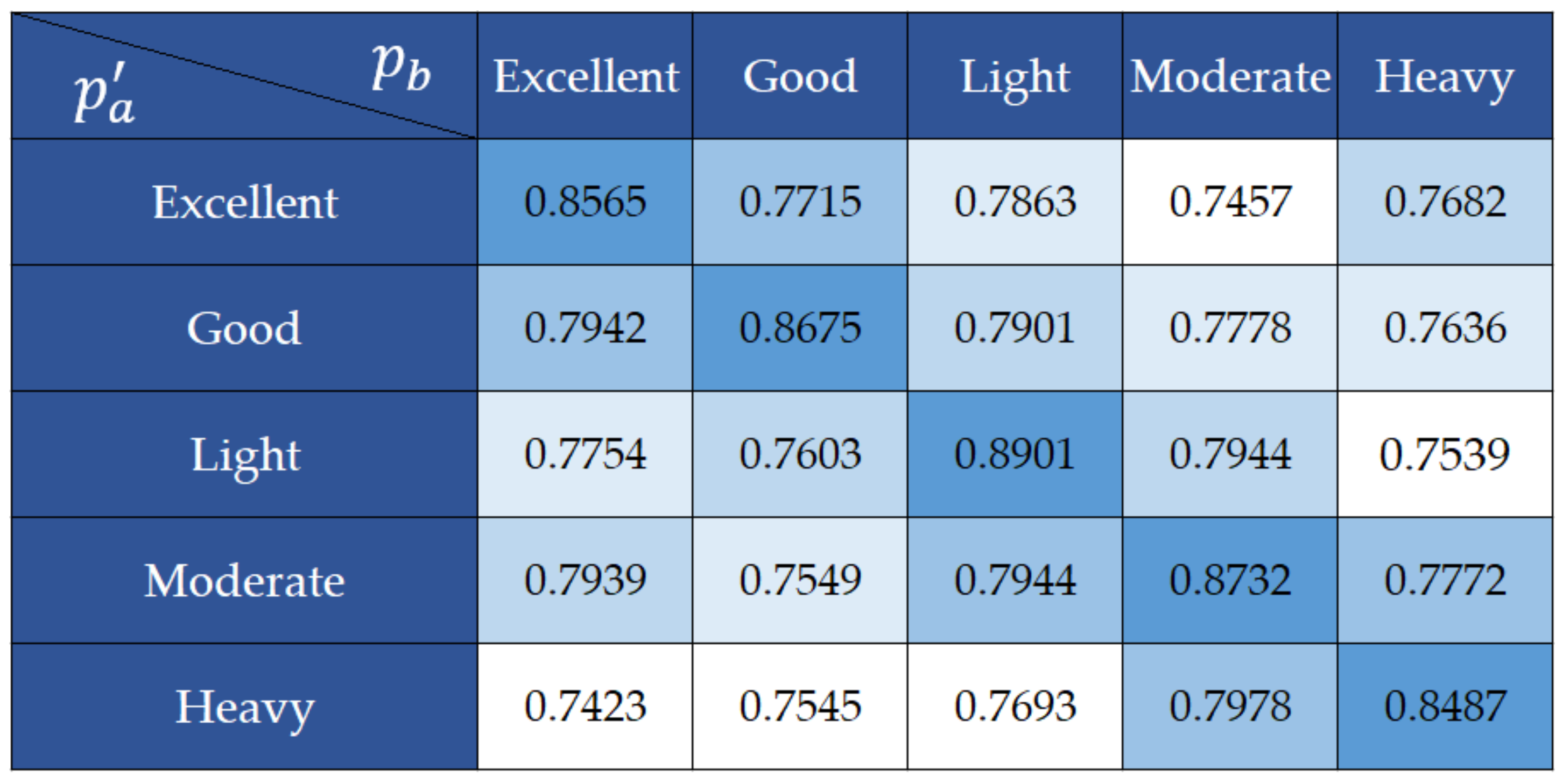
Figure 15 is a reference image, a matching image and a corrected image, from left to right, respectively. Since the air quality is high when the rating is excellent, the color correction result is not obvious. The color similarity of all corrected images is shown in Figure 16.
In Figure 16, p a represents a corrected image, and p b represents a reference image. By calculating the color similarity of the corrected image and the reference image, the color similarity at the same level is the largest. Compared with the color similarity before uncorrected, the color similarity between the same levels increased by 6.05%, 4.40%, 2.28%, 10.04%, and 1.45%, respectively. The color similarity between different levels of images is less than the color similarity under the same level.
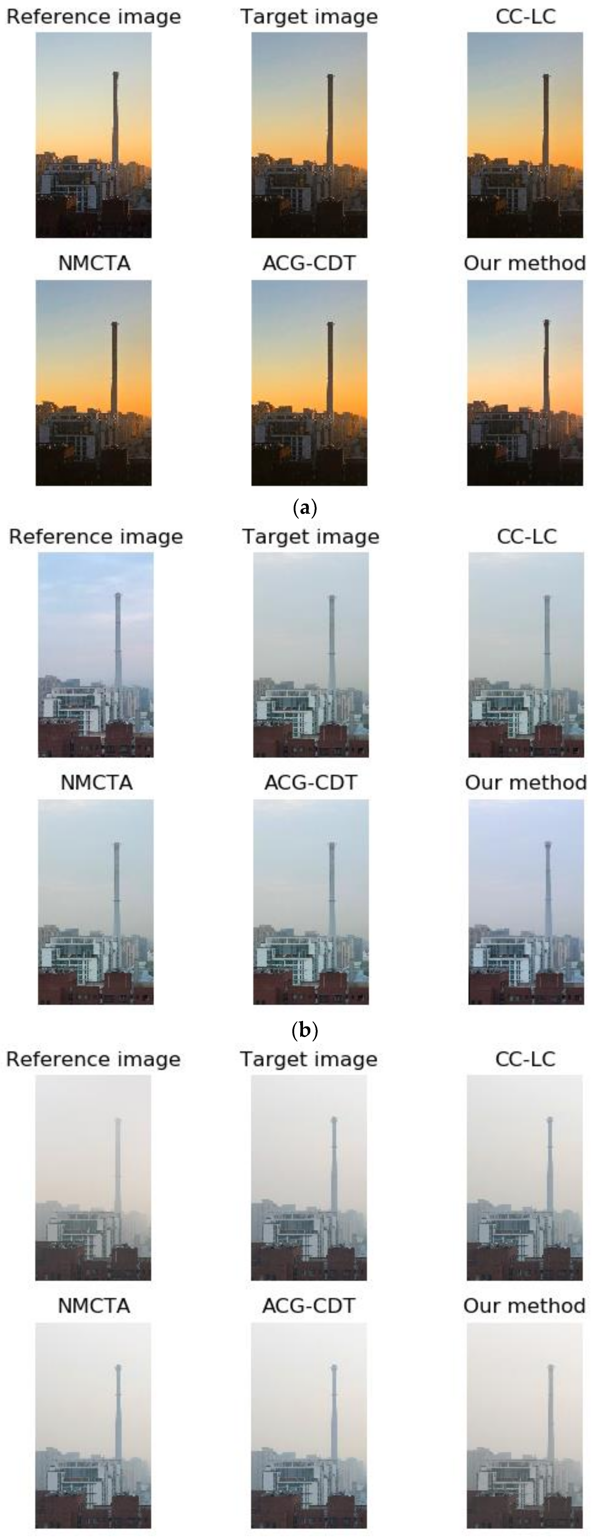
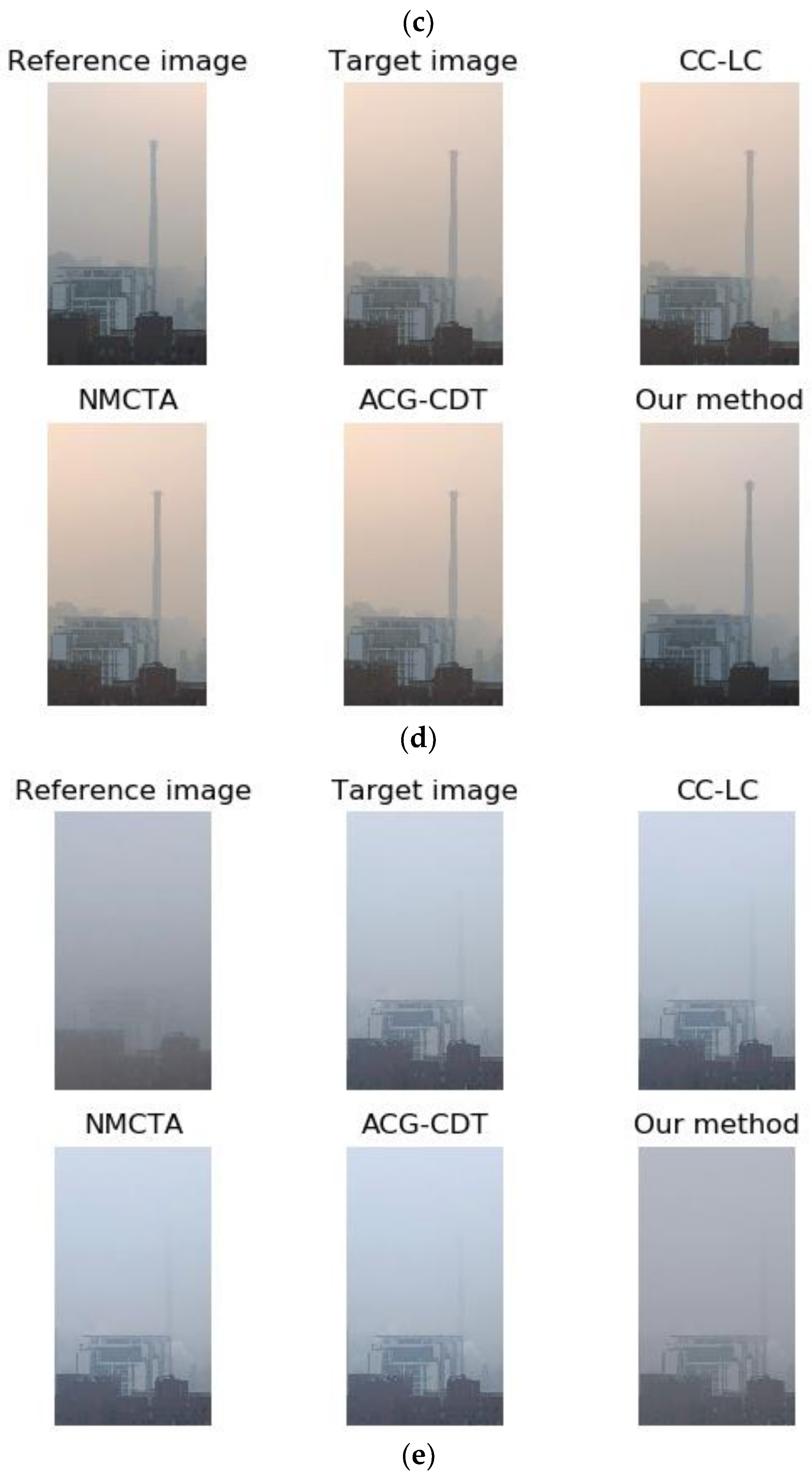
In order to further verify the validity of the color correction algorithm in this paper, color correction of stereo images using local correspondence (CC-LC) [10], Novel Multi-Color Transfer Algorithms and Quality Measure (NMCTA) [11], and ACG-CDT [17] are compared with the color correction algorithm in this paper. The comparison results are shown in Figure 17.
From Figure 17, the corrected image has a difference from the target image, and its color is closer to the reference image. Figure 17 shows the results of the correction of the images in the five levels. When the haze level is excellent and heavy, the correction result is more obvious; and when the haze level is light, the correction result is general. This shows that the color change of the image is closely related to the degree of haze. For color correction between the same level, the CC-LC, NMCTA, and ACG-CDT algorithms have limited ability to correct chromatic aberration. In general, the color correction algorithm of this paper is superior to other comparison algorithms.
In order to more objectively compare the effects of several color correction algorithms, this paper performs haze images recognition based on only changing the color correction algorithm. The experiment on the test set was repeated five times, and the accuracy of each time is shown in Figure 18.
According to five repeated experiments, the accuracy of the color correction method in this paper is about 85%; the accuracy of the unprocessed original image is the worst, only about 55%; the accuracy of other color correction algorithms is around 70%. Among them, the accuracy of CC-LC algorithm fluctuates the most, and the minimum accuracy and maximum accuracy are 58.6% and 77.1%, respectively. The average accuracy of the color correction algorithm in this paper is 14.1%, 16.5%, 19.9%, and 32.5% higher than the CC-LC, NMCTA, and ACG-CDT algorithms, respectively. In addition, the fluctuation of the accuracy of the color-corrected image is more stable by the lateral comparison of the five experiments. In summary, the result of the color correction algorithm in this paper is better in the comparison experiments.

3.4. Filter Comparison Experiments

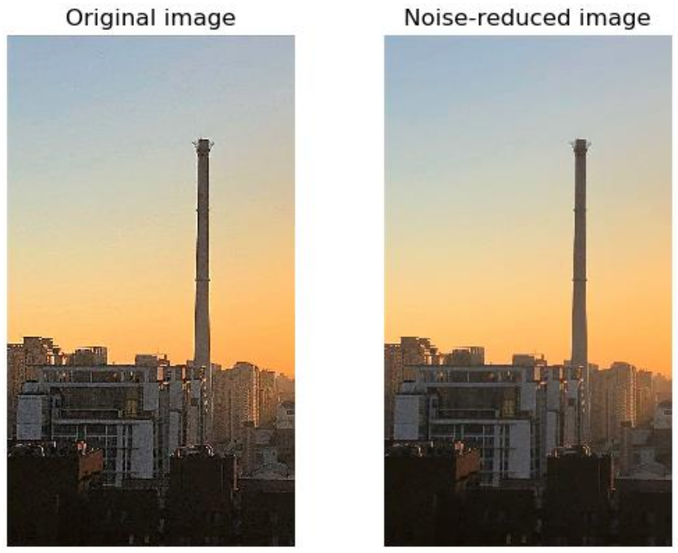
According to the study in Section 2.3, the improved Butterworth filter can effectively reduce the noise of the image. Taking the image at the level of excellent as an example, the filtered haze image is as shown in Figure 19.
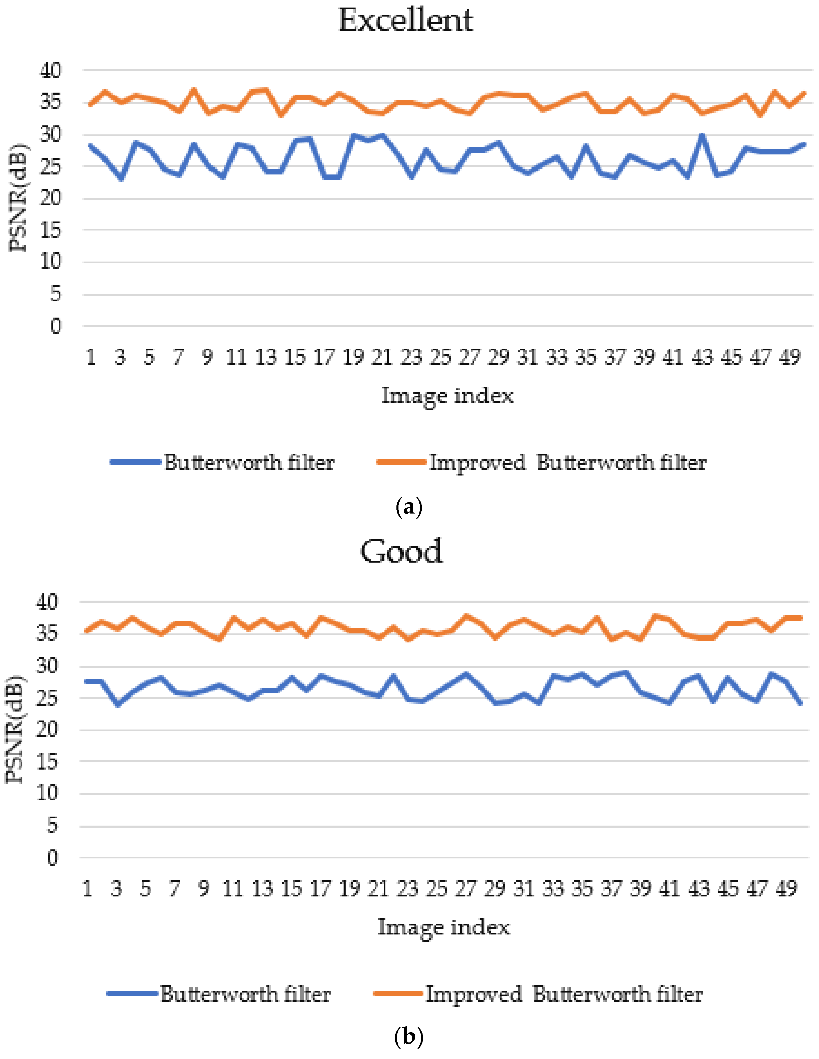
The noise-reduced image has fewer noise points than the original image, while retaining the key details of the image. In order to more intuitively test the effect of the improved Butterworth filter, this paper evaluates it using PSNR. The larger the value of PSNR, the higher the image quality, the smaller the effect of noise, and vice versa. The PSNR comparison results of the images before and after the improvement of the Butterworth filter are shown in Figure 20.
In this paper, 50 haze images from each haze level were randomly selected for display. It can be seen from Figure 20 that the original Butterworth filter has a low PSNR and a large PSNR fluctuation range; the improved Butterworth filter can significantly improve the PSNR of the image, and the PSNR fluctuation range is relatively stable. Compared to the original Butterworth filter, the improved Butterworth filter increases the average PSNR for each level by 33.60%, 35.91%, 35.26%, 40.72%, and 44.48%, respectively.
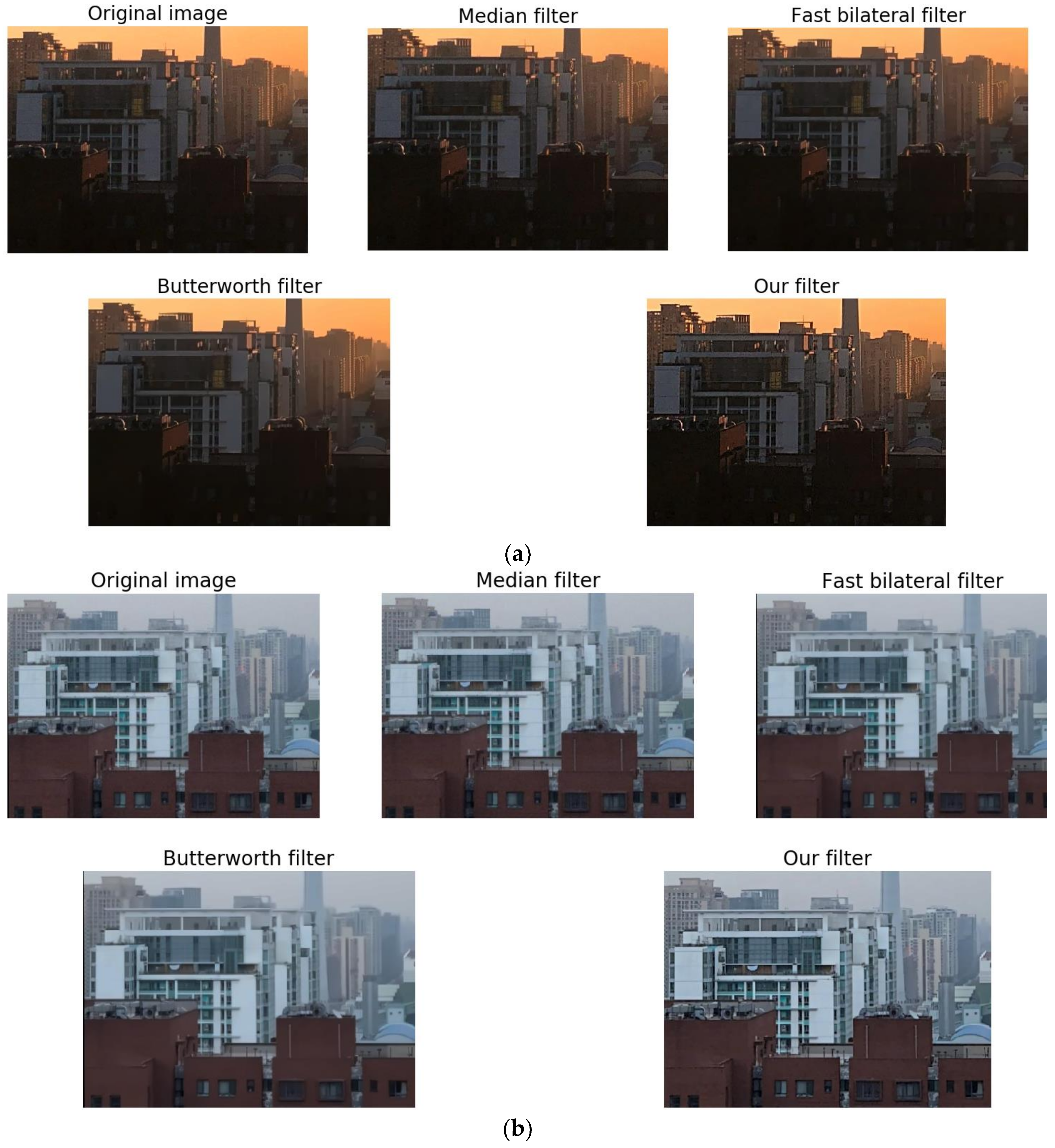
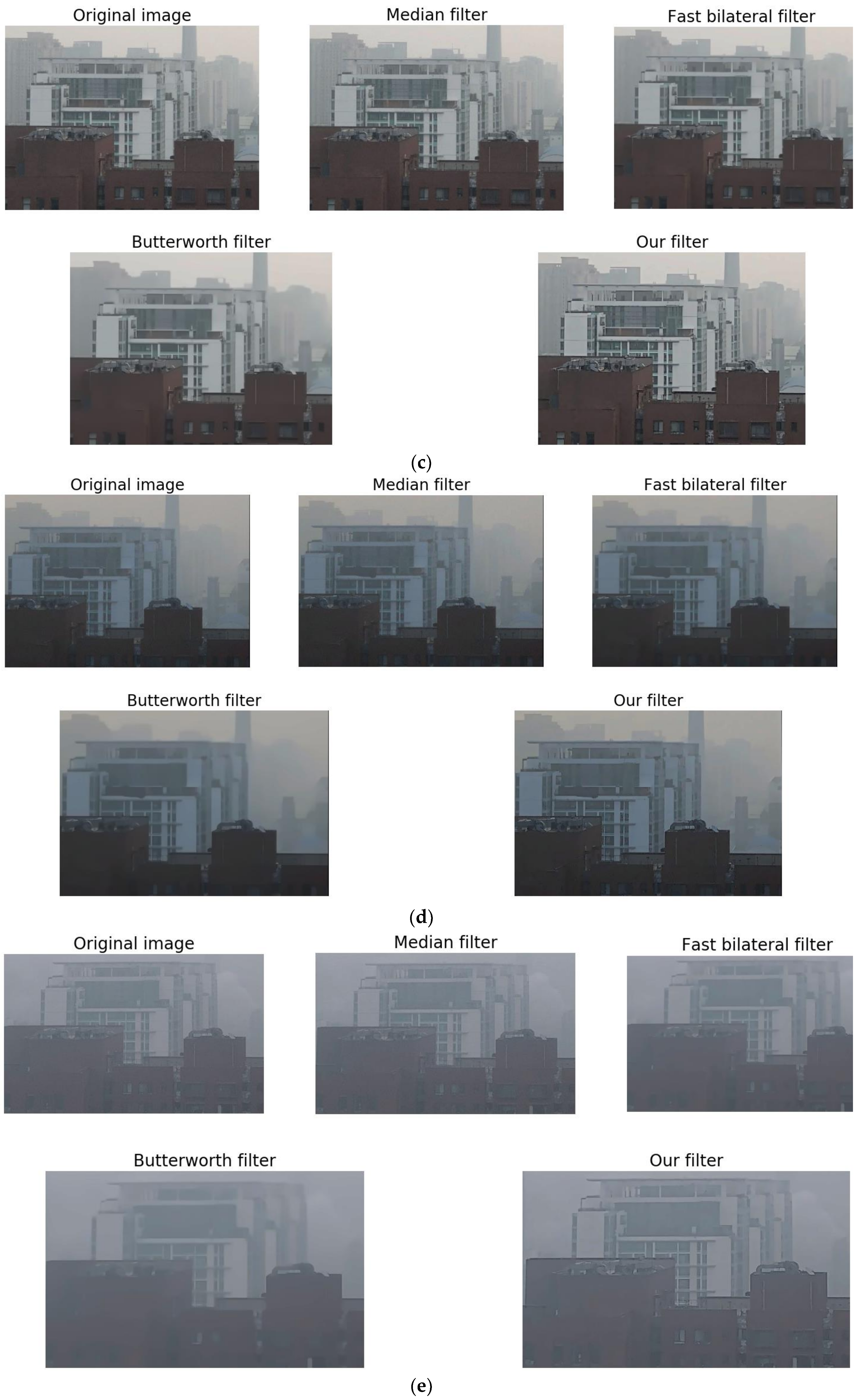
In order to verify the effectiveness of the improved Butterworth filter in this paper. This paper uses median filter [14], fast bilateral filter [15], and Butterworth filter [16] to compare with the filter of this paper. The image processed by the different filters is shown in Figure 21.
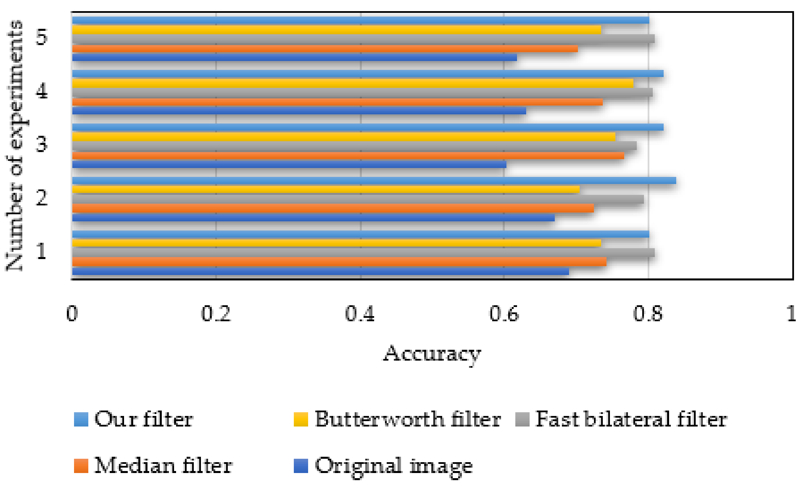
According to the results of Figure 21, the filter has the best noise reduction effect when the level is moderate and the level is heavy. Between each level, the improved Butterworth filter performs better than other filters. For example, in Figure 21b, the median filter, fast bilateral filter, and Butterworth filter all lose varying degrees of image detail when processing images. In contrast, the improved Butterworth filter in this paper preserves more image detail while reducing image noise. To further verify the effect of the improved filter, a comparison experiment was performed with only the filter changed. The results of the experiment are now shown in Figure 22.
It can be seen from the five repetitions of the experiment that the average accuracy of the original image without noise reduction is about 64%, and the accuracy of each experiment fluctuates around 13%. The noise reduction processing of the filter can improve the accuracy of the haze level recognition. The average accuracy of Butterworth filter, fast bilateral filter, median filter and our filter increased by 9.93%, 15.85%, 9.26%, 17.49%, respectively, compared to the average accuracy of the original image. Therefore, the improved Butterworth filter has a higher accuracy than the comparative filter.

3.5. Comparison Experiments of Identification Methods

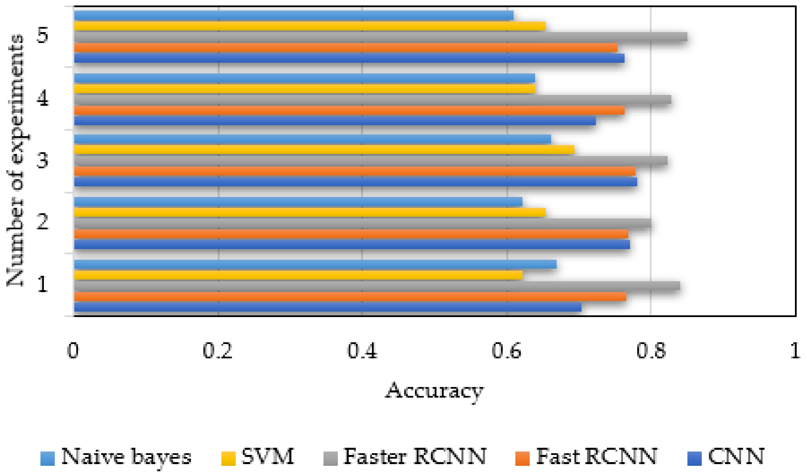
According to the study in Section 2.4, Faster R-CNN achieves the identification of haze levels by training haze images. In order to further verify the effectiveness of Faster R-CNN for haze level identification, this paper compares different identification methods to test. In the comparative experiments, CNN [4], Fast R-CNN [29], and Faster R-CNN are deep learning methods, and naive Bayes [32], and SVM [33] are traditional machine learning methods. The results after five repeated experiments are shown in Figure 23.
It can be seen from the five repetitions of the comparison experiments that the average accuracy of deep learning is 13.46% higher than the average accuracy of traditional machine learning. In CNN, Fast R-CNN, and Faster R-CNN, Faster R-CNN has the highest average accuracy. It is 7.94% higher than the average accuracy of CNN and 6.28% higher than the average accuracy of Fast R-CNN. In summary, Faster R-CNN performed better than other algorithms in the comparison experiments.

4. Conclusions and Discussion

This paper proposes a method of haze images recognition based on brightness optimization feedback and color correction, which solves the problem that the traditional technology cannot monitor the haze levels in an efficient and real-time method. Affected by factors such as light and shooting position, the haze images between the same level has obvious brightness difference and chromatic aberration. In order to solve the difference in brightness between the haze images in the same level, this paper uses the PSO algorithm to calculate the optimal parameters of image brightness correction. For the chromatic aberration between haze images in the same level, this paper corrects the chromatic aberration between images based on SURF algorithm and ACG-CDT [17] algorithm. In addition, since the corrected images still have noise, this paper improves the Butterworth filter according to the characteristics of the haze images. Finally, in order to realize the identification of haze levels, this paper trains the processed images based on Faster R-CNN. The effectiveness of this paper is verified by multiple sets of comparison experiments.
The research in this paper is mainly to identify the haze levels in the city. The images processed in the article are all from the open area with buildings. Therefore, the research in this paper does not involve the identification of haze levels in other cases. The identification of haze levels in small areas requires further research.

Author Contributions

S.H. performed the experiments, analyzed the data, wrote the paper; P.W. conceived and designed the experiments; Y.H. offered a lot of suggestions for paper writing.

Funding

This work was financially supported by the National Key R&D Program of China (no. 2017YFC0209901).

Conflicts of Interest

The authors declare no conflict of interest.

References

  1. Lipeng, L.; Bin, W.; Hui, L.; Xiaojun, W. Haze Pollution Level Detection Method Based on Image Gray Differential Statistics. Comput. Eng. 2016, 42, 225–230. [Google Scholar]
  2. Dabo, J.; Xiao, F.; Yanxiao, C.; Heqiang, B.; Hongqiang, W. Measuring Dust Amount of Open-pit Blasting Based on Image Processing. Eng. Blasting 2017, 23, 34–38. [Google Scholar]
  3. Zhang, H.; Ma, J. Simulation on Judgment Model of Air Pollution Degree Based on Image Processing. Comput. Simul. 2016, 33, 452–455. [Google Scholar]
  4. Yan, G.; Yu, M.; Shi, S.; Feng, C. The recognition of traffic speed limit sign in hazy weather. J. Intell. Fuzzy Syst. 2017, 33, 873–883. [Google Scholar] [CrossRef]
  5. Jiang, X.; Sun, J.; Ding, H.; Li, C. Video Image De-fogging Recognition Algorithm based on Recurrent Neural Network. IEEE Trans. Ind. Inform. 2018, 14, 3281–3288. [Google Scholar] [CrossRef]
  6. Wan, M.; Gu, G.; Qian, W.; Ren, K.; Chen, Q.; Maldague, X. Infrared Image Enhancement Using Adaptive Histogram Partition and Brightness Correction. Remote Sens. 2018, 10, 682. [Google Scholar] [CrossRef]
  7. Wang, A.; Wang, W.; Liu, J.; Gu, N. AIPNet: Image-to-Image Single Image Dehazing With Atmospheric Illumination Prior. IEEE Trans. Image Process. 2019, 28, 381–393. [Google Scholar] [CrossRef] [PubMed]
  8. Abdullah-Al-Wadud, M.; Kabir, M.H.; Dewan, M.A.A.; Chae, O. A Dynamic Histogram Equalization for Image Contrast Enhancement. IEEE Trans. Consum. Electron. 2007, 53, 593–600. [Google Scholar] [CrossRef]
  9. Vickers, V.E. Plateau equalization algorithm for real-time display of high-quality infrared imagery. Opt. Eng. 1996, 35, 1921. [Google Scholar] [CrossRef]
  10. Lee, Y.H.; Lee, I.K. Colour correction of stereo images using local correspondence. Electron. Lett. 2014, 50, 1136–1138. [Google Scholar] [CrossRef]
  11. Panetta, K.; Bao, L.; Agaian, S. Novel Multi-Color Transfer Algorithms and Quality Measure. IEEE Trans. Consum. Electron. 2016, 62, 292–300. [Google Scholar] [CrossRef]
  12. Wang, D.W.; Han, P.F.; Fan, J.L.; Liu, Y.; Xu, Z.J.; Wang, J. Multispectral image enhancement based on illuminance-reflection imaging model and morphology operation. Acta Phys. Sin. 2018, 67, 21. [Google Scholar]
  13. Qi-Chong, T.; Cohen, L.D. A variational-based fusion model for non-uniform illumination image enhancement via contrast optimization and color correction. Signal Process. 2018, 153, 210–220. [Google Scholar]
  14. Gang, L.I.; Fan, R.X. A New Median Filter Algorithm in Image Tracking Systems. J. Beijing Inst. Technol. 2002, 22, 376–378. [Google Scholar]
  15. Gunturk, B.K. Fast bilateral filter with arbitrary range and domain kernels. IEEE Trans. Image Process. A Publ. IEEE Signal Process. Soc. 2011, 20, 2690–2696. [Google Scholar] [CrossRef] [PubMed]
  16. Wang, D.H. Image processing method using mixed non-linear Butterworth filter. Comput. Eng. Appl. 2010, 46, 195–198. [Google Scholar]
  17. Pitié, F.; Kokaram, A.C.; Dahyot, R. Automated colour grading using colour distribution transfer. Comput. Vis. Image Underst. 2007, 107, 123–137. [Google Scholar] [CrossRef]
  18. Ren, S.; Girshick, R.; Girshick, R.; Sun, J. Faster R-CNN: Towards Real-Time Object Detection with Region Proposal Networks. IEEE Trans. Pattern Anal. Mach. Intell. 2017, 39, 1137–1149. [Google Scholar] [CrossRef] [PubMed] [Green Version]
  19. Xing, L.; Zeng, H.; Zhangkai, N.; Jing, C.; Canhui, C. Contrast-Changed Image Quality Assessment Method. J. Signal Process. 2017, 33, 319–323. [Google Scholar]
  20. Wang, L.; Zhao, Y.; Jin, W. Real-time color transfer system for low-light level visible and infrared images in YUV color space. Proc. SPIE Int. Soc. Opt. Eng. 2007, 6567, 65671G. [Google Scholar]
  21. Reinhard, E.; Stark, M.; Shirley, P.; Ferwerda, J. Photographic tone reproduction for digital images. Proc. ACM Trans. Graph. 2002, 21, 267–276. [Google Scholar]
  22. Gonzalez, R.C.; Woods, R.E. Digital Image Processing, 3rd ed.; Prentice Hall International: Upper Saddle River, NJ, USA, 2008; pp. 150–157. [Google Scholar]
  23. Shanmugavadivu, P.; Balasubramanian, K.; Muruganandam, A. Particle swarm optimized bi-histogram equalization for contrast enhancement and brightness preservation of images. Vis. Comput. 2014, 30, 387–399. [Google Scholar] [CrossRef]
  24. Guanghai, L.; Zuoyong, L. Content-Based Image Retrieval Using Three Pixels Color Co-Occurrence Matrix. Comput. Sci. Appl. 2012, 2, 84–89. [Google Scholar]
  25. Xie, J.T.; Wang, X.H. A Measurement of Color Similarity Based on HSV Color System. J. Hangzhou Dianzi Univ. 2008, 28, 63–66. [Google Scholar]
  26. Alain, H.; Ziou, D. Image Quality Metrics: PSNR vs. SSIM. In Proceedings of the 2010 20th International Conference on Pattern Recognition, Istanbul, Turkey, 23–26 August 2010; pp. 2366–2369. [Google Scholar]
  27. Wendi, W.; Xin, B.; Deng, N.; Li, J.; Liu, N. Single Vision Based Identification of Yarn Hairiness Using Adaptive Threshold and Image Enhancement Method. Measurement 2018, 128, 220–230. [Google Scholar]
  28. Tavakoli, A.; Mousavi, P.; Zarmehi, F. Modified algorithms for image inpainting in Fourier transform domain. Comput. Appl. Math. 2018, 37, 5239–5252. [Google Scholar] [CrossRef]
  29. Girshick, R. Fast R-CNN. In Proceedings of the IEEE International Conference on Computer Vision (ICCV), Santiago, Chile, 7–13 December 2015. [Google Scholar]
  30. He, K.; Zhang, X.; Ren, S.; Sun, J. Deep Residual Learning for Image Recognition. In Proceedings of the 2016 IEEE Conference on Computer Vision and Pattern Recognition, Las Vegas, NV, USA, 27–30 June 2016. [Google Scholar]
  31. Li, H.; Wang, J.; Li, R.; Lu, H. Novel analysis–forecast system based on multi-objective optimization for air quality index. J. Clean. Prod. 2018, 208, 1365–1383. [Google Scholar] [CrossRef]
  32. Da Silva, N.F.; Hruschka, E.R.; Hruschka, E.R., Jr. Tweet sentiment analysis with classifier ensembles. Decis. Support Syst. 2014, 66, 170–179. [Google Scholar] [CrossRef]
  33. Muñoz-Marí, J.; Gómez-Chova, L.; Camps-Valls, G.; Calpe-Maravilla, J. Image classification with semi-supervised one-class support vector machine. Image Signal Process. Remote Sens. XIV 2008, 7109, 71090B. [Google Scholar]
Figure 1. Implementation steps of this article.
Information 10 00081 g001
Figure 2. Reference images and target images.
Information 10 00081 g002
Figure 3. Technical route.
Information 10 00081 g003
Figure 4. Transform to YUV. From left to right are reference image in RGB. target image in RGB, reference image in YUV and target image in YUV.
Information 10 00081 g004
Figure 5. Brightness histogram of reference images and target images. (a) is a contrast histogram with the level of excellent; (b) is a contrast histogram with the level of good; (c) is a contrast histogram with the level of light; (d) is a contrast histogram with the level of moderate; (e) is a contrast histogram with the level of heavy.
Information 10 00081 g005aInformation 10 00081 g005bInformation 10 00081 g005c
Figure 6. Image matching. (a) is the result of a matching image with a level of excellent; (b) is the result of a matching image with a level of good; (c) is the result of a matching image with a level of light; (d) is the result of a matching image with a level of moderate; (e) is the result of a matching image with a level of heavy.
Information 10 00081 g006aInformation 10 00081 g006bInformation 10 00081 g006c
Figure 7. Traditional Butterworth filter function.
Information 10 00081 g007
Figure 8. Marked image.
Information 10 00081 g008
Figure 9. Region proposal network (RPN).
Information 10 00081 g009
Figure 10. Average brightness.
Information 10 00081 g010
Figure 11. Contrast before and after brightness correction. (a) is a histogram comparison before and after brightness correction when the level is excellent; (b) is a histogram comparison before and after brightness correction when the level is good; (c) is a histogram comparison before and after brightness correction when the level is light; (d) is a histogram comparison before and after brightness correction when the level is moderate; (e) is a histogram comparison before and after brightness correction when the level is heavy.
Information 10 00081 g011aInformation 10 00081 g011bInformation 10 00081 g011c
Figure 12. Comparison of different brightness correction methods. (a) is the comparison of different algorithms when the level is excellent; (b) is the comparison of different algorithms when the level is good; (c) is the comparison of different algorithms when the level is light; (d) is the comparison of different algorithms when the level is moderate; (e) is the comparison of different algorithms when the level is heavy.
Information 10 00081 g012aInformation 10 00081 g012b
Figure 13. Accuracy of different brightness correction methods on the test set.
Information 10 00081 g013
Figure 14. Color similarity between reference images and matching images.
Information 10 00081 g014
Figure 15. Color correction of matching image and reference image.
Information 10 00081 g015
Figure 16. Color similarity between reference images and corrected matching images.
Information 10 00081 g016
Figure 17. Comparison of different color correction methods. (a) is the comparison of different algorithms when the level is excellent; (b) is the comparison of different algorithms when the level is good; (c) is the comparison of different algorithms when the level is light; (d) is the comparison of different algorithms when the level is moderate; (e) is the comparison of different algorithms when the level is heavy.
Information 10 00081 g017aInformation 10 00081 g017b
Figure 18. Accuracy of different color correction methods on the test set.
Information 10 00081 g018
Figure 19. Image before and after noise reduction.
Information 10 00081 g019
Figure 20. PSNR comparison of original Butterworth filter with improved Butterworth filter. (a) is the PSNR comparison when level is excellent; (b) is the PSNR comparison when level is good; (c) is the PSNR comparison when level is light; (d) is the PSNR comparison when level is moderate; (e) is the PSNR comparison when level is heavy.
Information 10 00081 g020aInformation 10 00081 g020b
Figure 21. Comparison of different filters. (a) is the filters comparison when level is excellent; (b) is the filters comparison when level is good; (c) is the filters comparison when level is light; (d) is the filters comparison when level is moderate; (e) is the filters comparison when level is heavy.
Information 10 00081 g021aInformation 10 00081 g021b
Figure 22. Accuracy of different filters on the test set.
Information 10 00081 g022
Figure 23. Accuracy of different recognition methods on the test set.
Information 10 00081 g023
Table 1. Haze levels.
No.AQILevelNumber
I0–50Excellent271
II51–100Good674
III101–150Light705
IV151–200Moderate231
V>200Heavy219
Table 2. Particle initialization.
Particle indexInitial position of excellentInitial position of goodInitial position of lightInitial position of moderateInitial position of heavy
10.54870.41720.54870.54920.5486
20.71480.71990.71480.71580.7143
30.60260.00110.60260.60330.6024
40.54480.30270.54480.54520.5447
50.42380.14750.42380.42440.4241
60.64560.09320.64560.64690.6453
70.43770.18690.43770.43830.4378
80.89110.34590.89120.89110.8902
90.96270.39730.96270.96280.9618
100.38370.53870.38370.38430.3839
110.79110.41940.79110.79130.7906
120.52880.68480.52880.52930.5288
130.56790.20560.56790.56830.5678
140.92470.87740.92470.92480.9239
150.07190.02830.07190.07280.0728
Table 3. Parameter settings.
ParameterMeaningDefault Value
NParticle number15
t max Maximal iteration10
c 1 Learning factor2
c 2 Learning factor2
ω max Maximal intertia weight0.9
ω min Minimal intertia weight0.1
Table 4. Similarity of different histograms.
LevelReference image and target image (%)Reference image and corrected image (%)Degree of improvement (%)
Excellent7.3360.6053.27
Good72.3483.5711.23
Light79.1083.954.84
Moderate79.1984.285.09
Heavy28.1361.9933.86
Excellent7.3360.6053.27