Abstract
A power-down system has an on-state, an off-state, and a finite or infinite number of intermediate states. In the off-state, the system uses no energy and in the on-state energy it is used fully. Intermediate states consume only some fraction of energy but switching back to the on-state comes at a cost. Previous work has mainly focused on asymptotic results for systems with a large number of states. In contrast, the authors study problems with a few states as well as systems with one continuous state. Such systems play a role in energy-efficiency for information technology but are especially important in the management of renewable energy. The authors analyze power-down problems in the framework of online competitive analysis as to obtain performance guarantees in the absence of reliable forecasting. In a discrete case, the authors give detailed results for the case of three and five states, which corresponds to a system with on-off states and three additional intermediate states “power save”, “suspend”, and “hibernate”. The authors use a novel balancing technique to obtain optimally competitive solutions. With this, the authors show that the overall best competitive ratio for three-state systems is and the authors obtain optimal ratios for various five state systems. For the continuous case, the authors develop various strategies, namely linear, optimal-following, progressive and exponential. The authors show that the best competitive strategies are those that follow the offline schedule in an accelerated manner. Strategy “progressive” consistently produces competitive ratios significantly better than 2.
1. Introduction
With the shift towards renewable energy sources, such as biomass, wind, and solar on the power supply side and smart appliances and electric vehicles on the load side, there are enormous challenges in designing a reliable, effective and secure power infrastructures. Today, when renewables produce a surplus of energy, the surplus generally does not affect the operation of traditional power plants. Instead, renewables are throttled down or the surplus is simply ignored. In the future, it is projected that more than two-thirds of all domestic power will be generated by renewables and then this situation will not be tenable. Instead, the traditional power plants will need to be throttled down. Powering down a major power plant is not trivial and requires considerable extra cost—as noted in the authors’ recent paper on managing a renewable energy infrastructure [1].
Power management and energy-efficiency are also important topics in information technology itself, given the exponential growth in the number of information technology devices and cloud services worldwide. Finite state systems are used in electronic control, such as power optimization for laptop computers, hand-held devices, and work stations [2,3,4,5]. Eric Smith, Google’s former Chief Executive Officer, remarked “What matters most to the computer designers at Google is not speed but power, low power, because data centers can consume as much energy as a city" (Quote attributed to [6]) and energy costs at Google routinely exceed hardware costs [7]. Ways to minimize energy consumption are crucial and power usage has increasingly become a first order constraint in Information Technology. There is now a body of work on algorithmic approaches for energy efficiency (e.g., see Albers et al. for a survey [8]), but it is surprising that for power-down mechanisms only a few algorithmic techniques exist. The problems the authors study in this paper have been previously addressed only in an asymptotic sense, where the number of states is large (see [9,10]). In contrast, the authors here study problems with a few states as well as systems with one continuous state. Thus, a gap remains for obtaining exact results for specific systems, especially in renewable energy management, and this study addresses this gap.
1.1. Problem Formulation
The power-down problem is formally defined as follows: consider here a system which has two states, called ON, OFF, and additionally a continuous or finite set of intermediate states. In the continuous case, the set of states is , where the value 0 is mapped to the ON-state; the value 1 is mapped to the OFF state; and the interval is mapped to the intermediate states. The running cost of the device in the ON state is proportional to the time of usage and the device in the OFF state consumes zero amount of energy; the intermediate states serve as sleep states, where the running cost is also proportional to time, but a smaller cost . There is no cost to switching from ON to OFF or any of the intermediate states, but a fixed cost occurs when switching from any of the intermediate states to ON, with c the cost of switching from OFF to ON. For systems with a finite number of states, instead of mapping from , the states are in , with 0 being the ON-state, k being the OFF-state, and costs then described as , for —such a system is called a state system. The simplest of such systems is a two-state system where there is only OFF and ON, i.e., .
1.2. Previous Work, Contribution, and Organization of the Paper
The authors study problems in the framework of online competitive analysis, a comprehensive introduction to such analysis can be found in [11]. In the online model, an algorithm must make decisions without any knowledge of future inputs. The authors analyze online algorithms in terms of competitiveness, a measure of performance which compares the solution obtained online with the optimal offline solution for the same problem, where the lowest possible competitiveness is best. This model has the advantage that statistical assumptions are not necessary. The existing grid has been remarkably successful and reliable, which can be attributed to the accurate modeling of load pattern on the grid to accurately predict the demand. The demand prediction allows power generation to be easily adapted to the predicted demand; see the authors’ paper [1] for a survey on dependable electrical grids. However, the situation is markedly different with renewables because short-term gaps in renewable energy supply are hard to predict. As a result, the worst case analysis (i.e., not using forecasting or distributional assumptions) is more appropriate for a a truly resilient grid; worst case analysis gives a performance guarantee in the absence of reliable forecasting. For example, predictions are tenuous, as there have been extreme weather patterns in recent years, suspected by some climate scientists [12] to be related to a change in the Arctic Oscillation (OA) and North Atlantic Oscillation (NAO).
The online power-down problem with two states is equivalent to the noted “ski-rental problem”, which was first studied by Karlin et al. [13] to model caching in multi-processor systems. The relevance of the ski-rental problem for power-down is mentioned in [14] as well as in the survey article on energy efficient algorithms by Albers [8]; the authors will discuss the power-down equivalence further in Section 2. A randomized version of the problem was studied by [15] in connection with Dynamic TCP Acknowledgement.
The authors also mention that, for two-state power down problems, Bein et al. [16,17] have introduced the decrease-and-reset technique, which decreases the standby time gradually when the frequency of requests becomes low. In the decrease and reset approach, a parameter called “slackness degree” is introduced, which represents the frequency of arrivals; a near optimal algorithm can be constructed, which has superior competitiveness in the presence of slackness. It is noted that this approach is reliant on statistical assumptions and the authors do not pursue this approach in this paper.
Online multi-state systems were first studied in an asymptotic sense for systems with a large number of states by Augustine, Irani and Swami in [9,10]. They gave an algorithm to produce an approximation strategy and also a simple algorithm that achieves a competitive ratio of . There is much related work on speed scaling of processors [8]. This technique saves energy by throttling down the speed of a processor whenever possible, e.g., [18,19,20]. Chen et al. [21] consider the problem of online dynamic power management which provides hard real-time guarantees for multi-processor systems and Albers et al. [22] give multi-processor speed scaling with migration. This is part of a large body of work on scheduling jobs online on parallel machines with hard deadlines, see [23] for recent results. Other research considered power-down problems over a network to reduce the energy cost of idling server machines while maintaining an effective network [2,3,4,5]. This is part of a larger theme of using power management to achieve energy savings in data centers; see the authors’ recent article [24] as well as [25].
The work by Augustine et al. [9,10] is closest to the authors’ work, but here the focus is on systems with a small number of finite states as well as systems with one continuous state. Such systems play a role in energy efficiency and renewable energy management. The purpose of this paper is to fill the gap between asymptotic techniques and exact solutions for systems with states. The authors present here a novel balancing technique, and note that these techniques are markedly different from those in previous work. The authors obtain optimal and closed form solutions and report new results for numerous power-down systems. It is known that a simple strategy for the ski-rental problem yields a competitive ratio of 2 (see e.g., [13] or textbook [11]). The authors show that the overall best competitive ratio for three-state systems is and they obtain optimal ratios for various five state systems. For the continuous case, the authors develop various strategies, namely linear, optimal-following, progressive and exponential. The authors show that best competitive strategies are those that follow the offline schedule in an accelerated manner; strategy “progressive” consistently produces competitive ratios significantly better than 2.
The paper is organized as follows: in Section 2, the authors provide details of the online model, and show its relevance to energy efficiency and renewable energy management. The authors continue in Section 3 to analyze three-state systems and generalize such analysis in Section 4 for the situation of five states. Five state systems are inspired by devices used in everyday life, where there is the ON and OFF state and then three intermediate states “power save”, “suspend”, and “hibernate”. Based on these techniques in that section, the authors also outline a heuristic which works well for more than five states. In Section 5, the authors present the continuous model, and focus on five online power-down strategies: linear, optimal-following, progressive, logarithmic and exponential. Section 6 presents the conclusions.
2. Online Computation and the Smart Grid
In simulation and modeling, frequently statistical or distributional assumptions are made; for the power-down problem, models make assumptions about the distribution of requests. For example, in the traditional power power grid, the demand for power can be predicted throughout the day, and across the seasons, power demand can be predicted with a certain degree of certainty [26]. With renewable and decentralized power supplies, such predictions are much more precarious. Here, the competitive ratio is useful as a guarantee no matter how unusual the situation becomes.
Online algorithms make decisions without knowledge of future input. For the power-down problem, this means that an online algorithm will decide at each moment how to switch states without knowing what the next request will be. In contrast, an offline algorithm can make decisions based on the full knowledge of the entire input sequence. For example, algorithm A has competitive ratio C for a given request sequence , if
with the cost of A to serve , and the cost of the optimal offline algorithm on . If this is true for all feasible input sequences, then we say that the online algorithm is C-competitive. The competitive ratio for a given algorithm A is defined as the smallest such C possible. It is desirable to find the the online algorithm with the smallest competitive ratio, which is also referred to as the competitive ratio of the problem. See [11] for a broad introduction to the theory of online algorithms.
Returning now to the formulation of the power-down problem, at any time, the device may be in any state but it must be turned to the ON state when service is requested. Let and be non-negative real values that represent requests for service between start of service times and end of the service times , . Note that holds. Thus, at time , the state of a device must be in ON until time . In between requests the device can remain in the ON state or go to the OFF state or any of the intermediate states. Note that if is very close to it may be inefficient to turn the device off. Instead it could be advantageous to keep the machine on or perhaps operate the device in any of the intermediate states. It is important that during usage, the device must be ON—both offline and online. Thus, under competitive analysis the length of the service is irrelevant—the issue is only whether the machine switches to a new state at time —and one can thus assume without loss of generality, those usage times of the device are infinitesimal. Therefore, it is necessary to redefine the input sequence as where and define a request sequence in terms of the arrival time of request i.
Under competitive analysis, for the two-state problem, an optimal online algorithm, here referred to as , is well known for this problem [13]: switches to ON at a service request. After the service, remains in ON to stand by for time c units—recall that c is the cost of switching from OFF to ON. This means that if another service is requested within the standby period, simply remains in state ON. Only if the waiting time is larger than c will go to OFF after a standby time of c. Algorithm is 2-competitive, which is optimal.
This situation is analogous to the noted ski rental problem [13]. In the ski rental problem, a “friend” invites an invitee to go skiing, where one can rent skis at cost $1 or purchase them at cost $, for some . Unlike the inviter, the invitee does not know how often he/she will be invited. Thus, the invitee has to decide how often to rent and when to buy. It is easy to see that the best competitive ratio of the invitee cost versus the inviter cost achievable by any online algorithm for the ski rental problem is 2; the strategy is to rent m times before buying. The ski rental problem is analogous to the two-state power-down problem in the following way; both problems are about when to commit to a higher cost in anticipation of future savings. In the ski-rental problem, this commitment is when buying skis, whereas, in the power-down problem, the commitment is to accept a (large one-time) switching-on cost when the system is next switched off.
3. Systems with Three States
In the three-state problem, the states are ON, OFF, and one intermediate state, or INT. In the definition of power-down systems, this means , i.e., the states are named {ON, INT, OFF}. For convenience, the authors assume that both the running cost in state ON, as well as the switching cost from OFF to ON are 1. Furthermore, the costs of state INT are referred to as a and d instead of and , since the index is redundant when there is only one intermediate state. The costs of the system are summarized in the Table 1 below:

Table 1.
A three-state power-down system with running cost a in the intermediate state INT and switching cost d to switch from INT to ON.
An online algorithm for this problems is fully described by specifying two switching times and which denote the switch times from state ON to state INT and then state INT to state OFF. In contrast, the optimal offline algorithm is described by two values and as follows: if the request arrives before , then will be in the ON state during the idle duration; if the request arrives between and , then will be in the INT state, and if the request arrives after , then will be in the OFF state. Thus, is defined as follows:
where the values of and for given a and d are according to the following theorem:
Theorem 1.
assigns and .
Proof.
The offline cost curves are , , and . The curve intersects with when ; before this time, the ON state yields the optimal cost and after this time, the INT state yields the optimal cost. The curve intersects with at . If the request arrives before , then from 0 to , the optimal cost is obtained using the cost curve which is the ON state; if the request arrives between to , then the optimal cost is obtained using the cost curve , which is the INT state, and if the request arrives at or after , the optimal cost curve is , which is the OFF state. Therefore, and .
If , it is easily verified that it is not advantageous to use INT. Therefore, the lemma follows. ☐
Recall that any online algorithm starts in the ON state, at some point switches to INT and then to OFF state as given by values for and . The cost of such an algorithm, , is
For such online algorithms, it is necessary to determine its and values as to minimize its competitive ratio.
Lemma 1.
For an online algorithm with minimal competitiveness, it is necessary that (a) and (b) .
Proof.
For (a), it is assumed that . If this is the case, such that . Then, the online algorithm stays in ON for , whereas the offline algorithm would have chosen to be in the intermediate state, thus incurring only a cost of . Therefore, there is the following competitive ratio:
The online and offline costs can be compared to get:
It is clear that as increases the competitive ratio increases, since the online costs increase at a faster rate than the offline cost.
To prove (b) again, assume the contrary, namely that , and therefore where . In this case, the online algorithm goes from ON to INT to OFF, whereas the offline algorithm remains in ON. Quantifying this behavior, the competitive ratio is:
or
As increases, the competitive ratio increases as well and . So now to show that must be true, one first assumes , so the competitive ratio would be . It is clear that as increases, the competitive ratio will increase linearly. Now assume to examine the competitive ratio if . So . The competitive ratio would be:
or
Once again, as increases, the competitive ratio is increases. Thus, when and both lead to contradictions because the competitive ratio will not be minimal in those cases; thus, to minimize the competitive ratio. ☐
From Lemma 1, the competitive ratio for a three-state system depends only on the value of , since and is fully determined by the values of a and d. Clearly, the maximum ratio between and occurs when has just changed states i.e., at and . Define and as the competitive ratios at and ; then and can be written as:
This is because the ratios at the two breaking points have to match. The goal is to minimize the worst case competitive ratio at the switching time values. The competitive ratio of the system will be . We have:
Lemma 2.
The competitive ratio for the three-state system is minimized when .
Proof.
First, assume and the competitive ratio is minimal. If now the value for would be decreased by an arbitrarily small constant such that is still preserved, the value for would increase, but the value for would decrease from (11) and (12), respectively. This leads to a contradiction because the competitive ratio was not minimal. If , the value of can be increased while still maintaining . This also leads to a contradiction, since, with the competitive ratio between and , the maximum of the two has decreased. ☐
For a three-state system, the values of a and d can be any value between 0 and 1, and, for convenience, set . From Lemma 2 to obtain the optimal competitive ratio, it is known that must be true. From Lemma 1, the value of is known, and setting is used to obtain the optimal value as follows:
Solving for , we obtain:
Using the value of , it is possible to substitute Equation (14), into or and that will yield the optimal competitive ratio given a value for a and d:
Using Equation (16), it is possible to give a value for , and search for the optimal a and d values that will minimize the competitive ratios. We obtain:
Theorem 2.
For a three-state system where , the best competitive ratio achievable is when and .
Proof.
Consider Equation (16) and compute the derivative with respect to d:
After simplifying the above expression, we get
Solving for d, we obtain , and , and with those values the competitive ratio is . ☐
Table 2.
Best competitive ratios (CR) together with the corresponding online algorithm for that ratio (defined by switching time values and ) for given parameter value .
Table 3.
Best competitive ratios (CR) together with the corresponding online algorithm for that ratio (defined by switching time values and ) for various values close to 1.
In Table 2 and Table 3 and Figure 1, if the optimal competitive ratios are found for several values; the overall optimal competitive ratio is obtained when . Based on those experimental results, one can see that for a three-state machine, the competitive ratio is optimal when . Such a system is called and “ideal system”. In practice, therefore, it is advantageous to choose a system with whenever possible, as in this case there is a power-down strategy with optimal competitive ratio of . If, for example, there is a degree of freedom in designing an intermediate state for a plant then the intermediate state should ideally be such that holds.
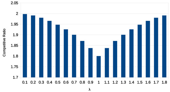
Figure 1.
Overall optimal competitive ratios for given values.
4. Systems with Few States
In this section, the authors consider systems with more than three-states, specifically with an arbitrary but small number of states. Generalizing from the three-state situation, for a -state situation, is fully described by values and the online Algorithm is fully described by values . Noting that the lemmas can be generalized inductively to a system with more than three-states, these are stated without proof:
Lemma 3.
For an online algorithms with minimal competitiveness, it is necessary that (a) and (b) .
Lemma 4.
For a state power-down system, the maximal competitive ratio appears at a transition, i.e., at a value in .
Lemma 5.
Given an online algorithm for a state power down problem with minimal competitive ratio . Then, .
Based on these lemmas, the authors present a heuristic for finding an optimally competitive algorithm. As in the three-state case, one can write the competitive ratio out at all transition points and use the fact from Lemma 5 that, in order for to be minimal, it must hold that , which yields the following system system of equations:
In the previous equations, the numerator reflects the fact that the online algorithms shifts down from state to state, whereas the denominator comes from the best choice available to the offline algorithm. Furthermore, as in the three-state case, these equations reflect the requirement that the ratios at the breaking points have to match.
The authors’ heuristic, which is detailed below, searches competitive ratios ; for each value considered, the corresponding values can be obtained by solving for in the previous system. It is shown in [10] that there exists a solution which has competitive ratio and this is taken as an initial solution. Next, given a desired precision , a competitive ratio search in the range ] is performed. This is guided by the following: if , the competitive ratio can only be minimal if due to Theorem 3; thus, must be reduced. If , then there there is no -competitive solution and must be increased. This process continues until ; a ratio arbitrarily close to optimal is obtained.
Algorithm 1 was used to model a typical system with few states, namely a quintuple system. Such a system is inspired by devices used in everyday life, where there is the ON and OFF state, and three intermediate states “power save”, “suspend”, and “hibernate”. The authors have simulated a system with running costs , , , and switching costs , , , , . The iterations of the simulation using Algorithm 1 are shown in Table 4.
Table 4.
Sample run of Algorithm 1: for each iteration, the current competitive ratio (CR) together with the the corresponding online algorithm for that ratio (defined by switching time values ) is shown.
| Algorithm 1 Power-down heuristic |
 |
Based on the value of , at each iteration, a new value for the competitive ratio between the upper bound and the lower bound is selected. The authors note that using Theorem 5 which implies the other values follow. Thus, a binary search on the competitive ratio in the range is performed, until a value such that is achieved. Figure 2 displays the situation from Table 4. Ratios are maximized at transition times, decreasing as the standby time moves away from any transition time until the next transition time is reached.
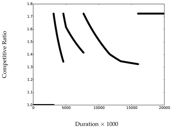
Figure 2.
The solution obtained in the sample run of Table 4. Per Lemma 4 at switching times, all ratios are equal.
The authors have conducted extensive simulations for various quintuple systems. Results are shown in Table 5.
Table 5.
Simulations results for various five-state systems (given by and parameter values) when . Competitive ratios are well below 2.
The authors note that the heuristic described here does not rely on asymptotic assumptions on a large number of states, in fact the heuristic is faster when there are few states as only few must be recalculated in each step. The heuristic is thus tailored to the situation of few states, unlike a meta-heuristic, or the technique in [9,10].
5. Continuous Models
5.1. Offline and Online Strategies
The authors now turn to the power-down problem with a continuous number of states. Such systems are quite useful in practice: power-down systems either feature a few intermediate states, up to five, perhaps, or a continuous number of states. The following model is used here: running costs are of the form and switching costs are modeled as , with given parameters a, d, . Figure 3 shows the model for , , . The techniques developed in this section can be generalized to various other models with continuous cost functions. In this section, offline and online strategies are conducted for these models.
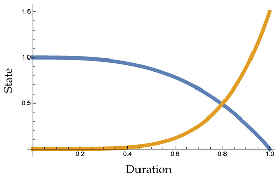
Figure 3.
(Brown) and (Blue) curves.
It is important to remember that the behavior of the offline algorithm has full clairvoyance, and thus has full knowledge of future idle times. With this clairvoyance, one can make use of the derivative of and derive . Seeking to minimize the cost from the start of the idle period to its end one, is obtained as the optimal cost for this system. From this, the threshold value, , is calculated, which denotes the time when the machine powers down completely. In the next Equation (22), the is set to the value 1, which denotes the state of the machine when it is fully powered off:
By setting to this state value, one can simply solve (22) to determine the value at which the machine is powered off; one obtains:
The authors now turn to online strategies. Given a strategy , there is an online cost
where the first term describes the accumulated run time as the online algorithms moves along states and the second term described the switching cost from the resulting state. As before in the discrete case, note that, unlike an offline algorithm, an online algorithm moves from an initial state to lower power states before the next request.
It is noted that the offline cost is simply given by the cost to be in the best state for the situation (first term) plus the switching cost (second term):
Generalizing the ski-rental strategy to the continuous case, one can define the “Lower Envelope” approach [10] where the online algorithms mimics offline behavior; thus, a first continuous version of the lower envelope strategy is given:
In Figure 4 and Figure 5, it can be seen that the competitive ratio increases as idle time passes. When this reaches the value of , the competitive ratio is the largest, with a competitive ratio of 2.
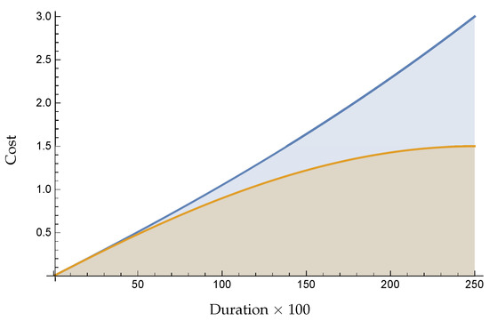
Figure 4.
Cost of OFFLINE (Brown) and ONLINE (Blue).
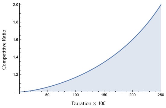
Figure 5.
Competitive ratio.
A key question is to explore the strategies that can improve this canonical competitiveness of 2. In other words, what are “better-than-2-competitive” strategies? To this end, the authors have investigated various online strategies. The primary idea is to decelerate or accelerate the online strategy as compared to offline. The strategies below are referred to as “linear”, “logarithmic”, “exponential”, and progressive due to their individual characteristics; in the definitions given, the values C, t, and z are control parameters to tune acceleration or deceleration of the various online strategies:
The authors show the strategies in Figure 6 and note that both the depicted linear and exponential strategies are below optimal offline which means that progress to lower power states is at a slower rate. Alternatively, logarithmic and progressive lie above the optimal offline; thereby, it is observed that the transition to lower power states is at faster rates than optimal offline.
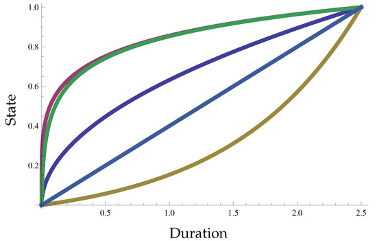
Figure 6.
(Brown), Linear (Blue), Strategy (Dark Blue), (Green), (Violet) strategy curves.
5.2. A Summary of Simulation Results
In this subsection, the authors give simulations results to gain insight into how these strategies perform with regards to competitiveness.
This starts with strategies that transition to lower states less aggressively: these are linear and exponential, see Figure 7 and Figure 8; and then looks to strategies with more aggressive transitioning, as in logarithmic, see Figure 9. For short idle periods, both linear and exponential show lower costs when juxtaposed to logarithmic. However, in the case of longer idle periods, when a request is similar to , logarithmic is best. It is clear that both linear and exponential would be sub-par here as these strategies remain in a higher power state for a longer stretch, resulting in wasted energy.
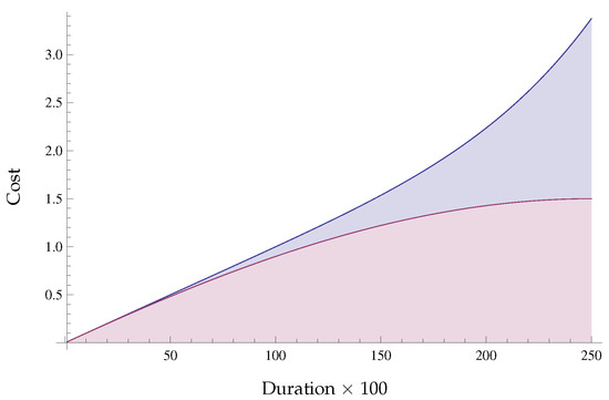
Figure 7.
Cost Linear(r) (Violet) and Cost OFFLINE (Purple).
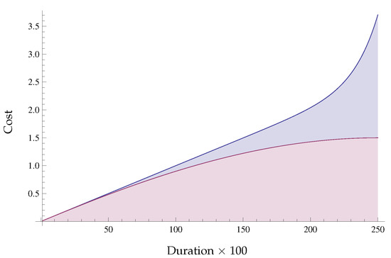
Figure 8.
Cost (Violet) and Cost OFFLINE (Purple).
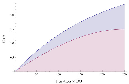
Figure 9.
Cost (Violet) and Cost OFFLINE (Purple).
Competitive ratios for linear, exponential and logarithmic are depicted in Figure 10, Figure 11 and Figure 12. Indeed, the competitive ratios validate what was noted above. Linear and exponential perform better for the beginning of the idle time compared to logarithmic, but soon they get worse as the idle duration increases. Thus, it is advantageous overall to power-down to lower power states at a faster rate than the offline curve.
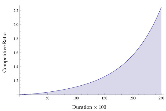
Figure 10.
Competitive ratio linear function.
Figure 11.
Competitive ratio .

Figure 12.
Competitive ratio .
Next is a host of examples for the progressive strategy.
In Figure 13, Figure 14 and Figure 15, for various parameter values t and z are given. Note that, if t and z are not too large, the online strategy goes to a lower power state more swiftly. Note that clearly the control parameters t and z can be used to control the rate at which the online strategy reaches smaller power states. Additionally, t causes a more significant impact on the function than the value of z since one can increased t by only a smaller amount than to have a dramatic effect. In the experimentation, the competitive ratios for a range of values t and z can be observed.
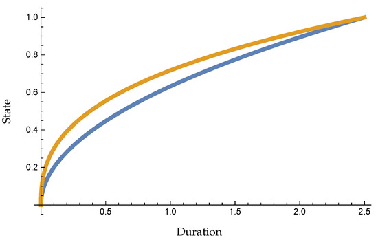
Figure 13.
Strategy OPT (Blue) and online strategies for , (Brown).
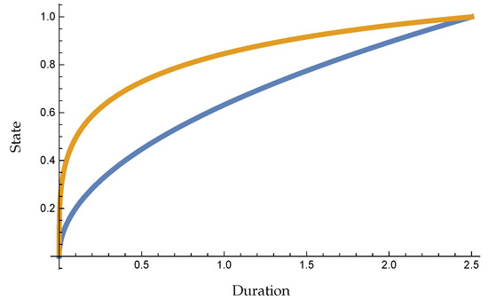
Figure 14.
Strategy OPT (Blue) and online strategies for , (Brown).
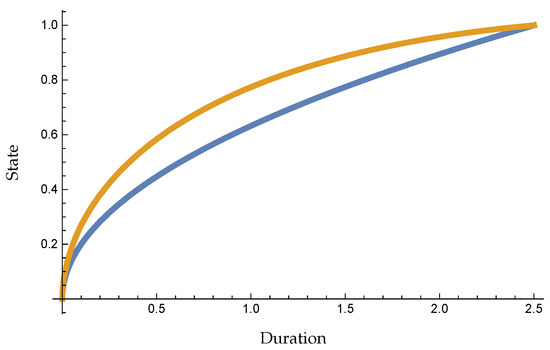
Figure 15.
Strategy OPT (Blue) and online strategies for , (Brown).
For progressive with a relatively small value of t, see Figure 16 and Figure 17. As with earlier strategies, the competitive ratio is smaller when the online strategy changes to a lower state more aggressively. Turning to Figure 18, one observes that ratios are larger when states are changed more slowly. Referring to Figure 13 and Figure 18, with a larger t value, progressive and offline strategy curves are rather congruent. This means that such an algorithm behaves more like the lower envelope. Next, larger values of z are analyzed.
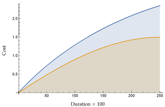
Figure 16.
Costs for , (Blue) and Cost OFFLINE (Brown).
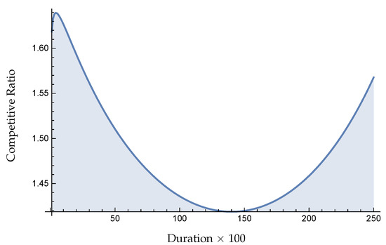
Figure 17.
Competitive ratio , .
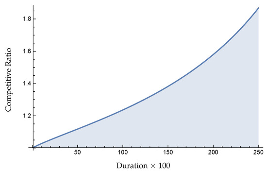
Figure 18.
Competitive ratio , .
Results are similar to what was observed before when t was increased. Ratios are worse (compare Figure 19 and Figure 20), but the required increase to z values for a similar effect is greater. Increasing z makes the ratio go up at a more linear rate, compared to increases of t; in addition, the competitive ratio is somewhat lower when the value of t is increased. Either way, increasing t or z, the authors approach a strategy more as offline, and thereby to lower envelope behavior. Moreover, raising t effects a more rapid change in the schedule, and results in a larger and worse competitive ratio than increases to z, although there is a long period during the idle duration where the competitive ratio is better for higher t values. Significantly, ratios are larger for larger t values. In Table 6, competitive ratios for various such parameter values are given. We conclude that it is advantageous to use fast acceleration through smaller values of t and z. However, Table 6 reveals that things are not monotonic. For example, for and a competitive ratio of results, whereas for the same z-value and the competitive ratio is significantly larger with a value of . Thus, careful analysis is required for each individual system.
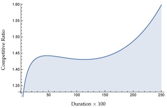
Figure 19.
Competitive ratio , .
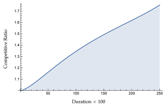
Figure 20.
Competitive ratio , .
Table 6.
Results for progressive for various parameters. Competitive ratios are well below 2.
6. Conclusions
Power-down problems with few states, as well as power-down problems with one continuous state, play an important role in energy-efficiency for both information technology and the management of renewable energy in a truly resilient electrical grid. The authors have shown that in both situations—a few discrete states or one continuous state—competitive strategies exist and that those strategies can be efficiently found in closed form or through heuristics. One general rule that emerges from this work is that, in order to obtain good competitive ratios, the online strategy needs to switch to lower power states at a faster rate than for the offline strategy. This general insight can be useful for developing strategies for idle and power up cost types other than those considered in this paper.
The work by the authors shows that, even under the worst-case competitive analysis, ratios of significantly below the value of 2 can be achieved. This means that quantitative quality guarantees for a resilient smart grid were provided by this work. Table 5 shows that for systems with five states, a competitive ratio of close to was achieved, i.e., significantly less than the best achievable value of for three-states (see Table 3). For a continuous system, it is clear from our studies that progressive strategies generally achieve the best results, e.g., close to in one case described in Table 6.
The authors suggest that such guarantees are crucial for policy makers as society transitions to a smart grid, which uses primarily renewable energy. A limitation of this study is that it does not address average case analysis, and it would be interesting in future work to perform simulation work to ascertain performance in practice for a smart grid as described in [1].
As mentioned in the Introduction, for discrete power down problems, Bein et al. [16,17] have introduced the decrease-and-reset technique, which decreases the standby time gradually when the frequency of the device usage becomes low. If we allow the worst-case competitive ratio to increase by only a small positive constant from the optimal value, we can design numerous algorithms other than the optimal strategy that can be designed (which are nonetheless “near optimal”). Next, the authors introduce a parameter called “slackness degree”, which represents the frequency of arrivals and can be constructed near optimal, which has superior competitiveness in the presence of slackness. Future work may consider applying decrease and reset in the continuous case as well.
Author Contributions
The three authors contributed equally to this paper. The order of authors is alphabetical.
Funding
The work of author Wolfgang Bein was supported by the National Science Foundation, Grant IIA 1427584. The work of author Hiro Ito was partially supported by CREST, JST, Grant No. JPMJCR1402 and KAKENHI, JSPS, Grant No. 15K11985.
Acknowledgments
The authors are grateful for the guidance given by Rüdiger Reischuk of Universität Lübeck during his sabbatical visit to the University of Nevada, Las Vegas, USA.
Conflicts of Interest
The authors declare no conflict of interest.
References
- Bein, W.; Madan, B.B.; Bein, D.; Nyknahad, D. Algorithmic Approaches for a Dependable Smart Grid. In Information Technology: New Generations: 13th International Conference on Information Technology; Latifi, S., Ed.; Springer: Berlin/Heidelberg, Germany, 2016; pp. 677–687. [Google Scholar]
- Agarwal, Y.; Hodges, S.; Chandra, R.; Scott, J.; Bahl, P.; Gupta, R. Somniloquy: Augmenting Network Interfaces to Reduce PC Energy Usage. In Proceedings of the 6th USENIX Symposium on Networked Systems Design and Implementation, Boston, MA, USA, 22–24 April 2009; USENIX Association: Berkeley, CA, USA, 2009; pp. 365–380. [Google Scholar]
- Agarwal, Y.; Savage, S.; Gupta, R. SleepServer: A Software-only Approach for Reducing the Energy Consumption of PCs Within Enterprise Environments. In Proceedings of the 2010 USENIX Conference on USENIX Annual Technical Conference, Boston, MA, USA, 22–25 June 2010; USENIX Association: Berkeley, CA, USA, 2010; p. 22. [Google Scholar]
- Nedevschi, S.; Chandrashekar, J.; Liu, J.; Nordman, B.; Ratnasamy, S.; Taft, N. Skilled in the Art of Being Idle: Reducing Energy Waste in Networked Systems. In Proceedings of the 6th USENIX Symposium on Networked Systems Design and Implementation, Boston, MA, USA, 22–24 April 2009; USENIX Association: Berkeley, CA, USA, 2009; pp. 381–394. [Google Scholar]
- Reich, J.; Goraczko, M.; Kansal, A.; Padhye, J. Sleepless in Seattle No Longer. In Proceedings of the 2010 USENIX Conference on USENIX Annual Technical Conference, Boston, MA, USA, 22–25 June 2010; USENIX Association: Berkeley, CA, USA, 2010; p. 17. [Google Scholar]
- Pruhs, K. Green computing algorithmics. In Proceedings of the 2011 IEEE 52nd Annual Symposium on Foundations of Computer Science (FOCS), Palm Springs, CA, USA, 22–25 October 2011; pp. 3–4. [Google Scholar]
- Barroso, L. The price of performance. ACM Queue 2005, 3, 48–53. [Google Scholar] [CrossRef]
- Albers, S. Energy-Efficient Algorithms. Commun. ACM 2010, 53, 86–96. [Google Scholar] [CrossRef]
- Augustine, J.; Irani, S.; Swamy, C. Optimal Power-Down Strategies. In Proceedings of the 45th Annual IEEE Symposium on Foundations of Computer Science, Rome, Italy, 17–19 October 2004; pp. 530–539. [Google Scholar]
- Augustine, J.; Irani, S.; Swamy, C. Optimal Power-Down Strategies. SIAM J. Comput. 2008, 37, 1499–1516. [Google Scholar] [CrossRef]
- Borodin, A.; El-Yaniv, R. Online Computation and Competitive Analysis; Cambridge University Press: Cambridge, UK, 1998. [Google Scholar]
- Hall, R.; Erdélyi, R.; Hanna, E.; Jones, J.M.; Scaife, A.A. Drivers of North Atlantic Polar Front jet stream variability. Int. J. Climatol. 2014. [Google Scholar] [CrossRef]
- Karlin, A.; Manasse, M.; Rudolph, L.; Sleator, D. Competitive snoopy caching. Algorithmica 1988, 3, 79–119. [Google Scholar] [CrossRef]
- Irani, S.; Pruhs, K.R. Algorithmic Problems in Power Management. SIGACT News 2005, 36, 63–76. [Google Scholar] [CrossRef]
- Karlin, A.R.; Kenyon, C.; Randall, D. Dynamic TCP Acknowledgement and Other Stories About e/(e-1). In Proceedings of the Thirty-third Annual ACM Symposium on Theory of Computing, Crete, Greece, 6–8 July 2001; ACM: New York, NY, USA, 2001; pp. 502–509. [Google Scholar]
- Andro-Vasko, J.; Bein, W.; Nyknahad, D.; Ito, H. Evaluation of Online Power-Down Algorithms. In Proceedings of the 12th International Conference on Information Technology—New Generations, Las Vegas, NV, USA, 13–15 April 2015; pp. 473–478. [Google Scholar]
- Bein, W.; Hatta, N.; Hernandez-Cons, N.; Ito, H.; Kasahara, S.; Kawahara, J. An Online Algorithm Optimally Self-tuning to Congestion for Power Management Problems. In Proceedings of the 9th International Conference on Approximation and Online Algorithms, Saarbrücken, Germany, 8–9 September 2011; pp. 35–48. [Google Scholar]
- Bansal, N.; Chan, H.L.; Lam, T.W.; Lee, K.L. Scheduling for speed bounded processors. In Proceedings of the 35th International Colloquium on Automata, Languages and Programming, Reykjavik, Iceland, 7–11 July 2008; pp. 409–420. [Google Scholar]
- Bansal, N.; Chan, H.L.; Pruhs, K.; Katz, D. Improved bounds for speed scaling in devices obeying the cube-root rule. In Proceedings of the 36th International Colloqium on Automata, Languages and Programming, Rhodes, Greece, 5–12 July 2009; pp. 144–155. [Google Scholar]
- Han, X.; Lam, T.W.; Lee, L.K.; To, I.K.K.; Wong, P.W.H. Deadline scheduling and power management for speed bounded processors. Theor. Comput. Sci. 2010, 411, 3587–3600. [Google Scholar] [CrossRef]
- Chen, J.J.; Kao, M.J.; Lee, D.; Rutter, I.; Wagner, D. Online dynamic power management with hard real-time guarantees. Theor. Comput. Sci. 2015, 595, 46–64. [Google Scholar] [CrossRef]
- Albers, S.; Antoniadis, A. Race to Idle: New Algorithms for Speed Scaling with a Sleep State. In Proceedings of the Twenty-third Annual ACM-SIAM Symposium on Discrete Algorithms, Kyoto, Japan, 17–19 January 2012; Society for Industrial and Applied Mathematics: Philadelphia, PA, USA, 2012; pp. 1266–1285. [Google Scholar]
- Anand, S.; Garg, N.; Megow, N. Meeting Deadlines: How Much Speed Suffices? In Proceedings of the ICALP 2011, Zurich, Switzerland, 4–8 July 2011.
- Bein, W. Energy Saving in Data Centers. Electronics 2018, 7, 5. [Google Scholar] [CrossRef]
- Dayarathna, M.; Wen, Y.; Fan, R. Data Center Energy Consumption Modeling: A Survey. IEEE Commun. Surv. Tutor. 2016, 18, 732–794. [Google Scholar] [CrossRef]
- Borges, C.E.; Penya, Y.K.; Fernández, I. Evaluating Combined Load Forecasting in Large Power Systems and Smart Grids. IEEE Trans. Ind. Inform. 2013, 9, 1570–1577. [Google Scholar] [CrossRef]


© 2019 by the authors. Licensee MDPI, Basel, Switzerland. This article is an open access article distributed under the terms and conditions of the Creative Commons Attribution (CC BY) license (http://creativecommons.org/licenses/by/4.0/).