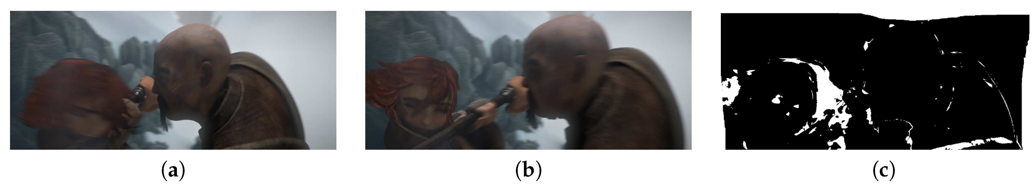
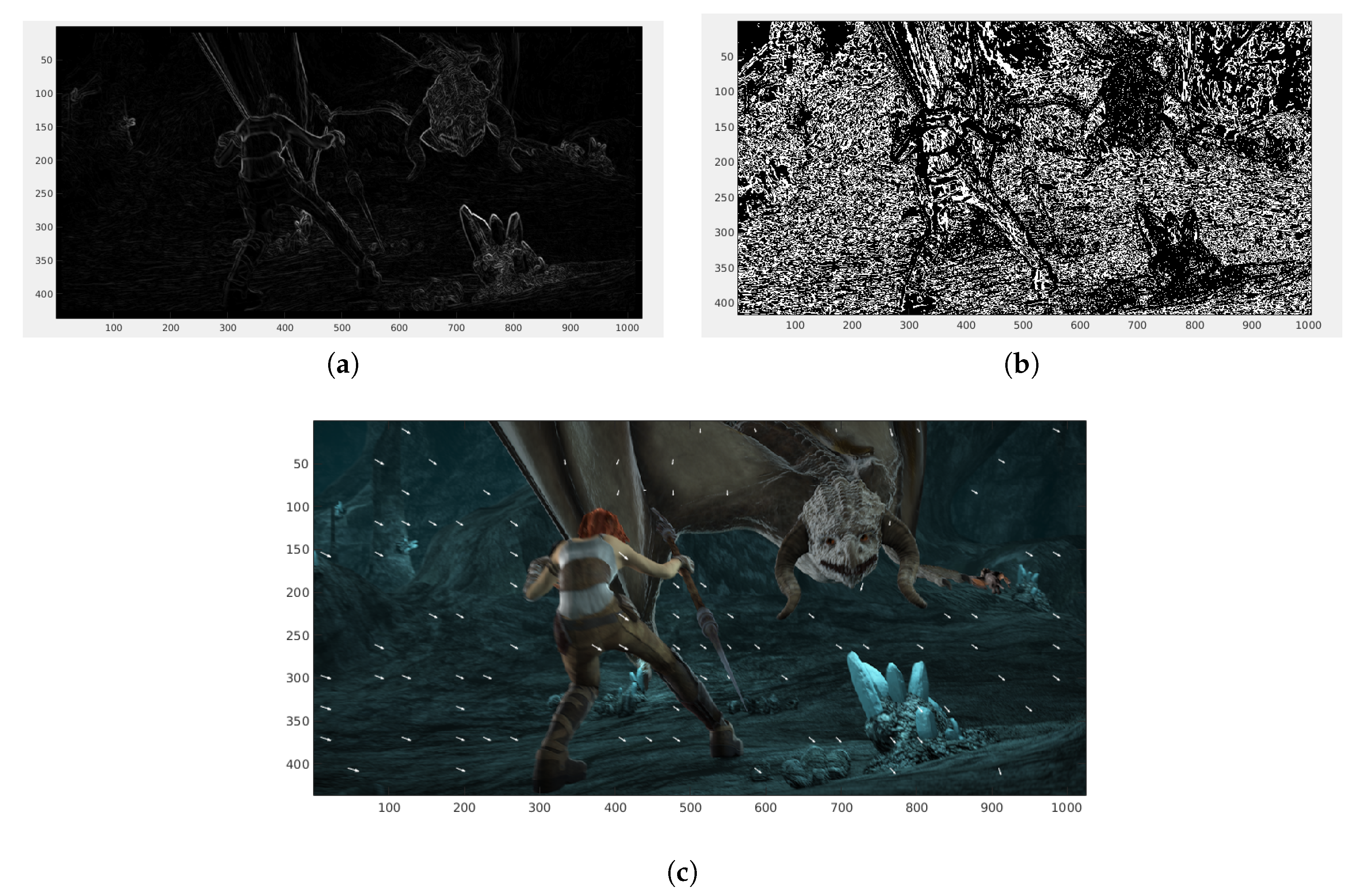
Figure 1.
Occlusion estimation comparing optical flow error with a threshold . (a) Frame_0049 of sequence ambush_5; (b) Frame_0050; (c) occlusion estimation.
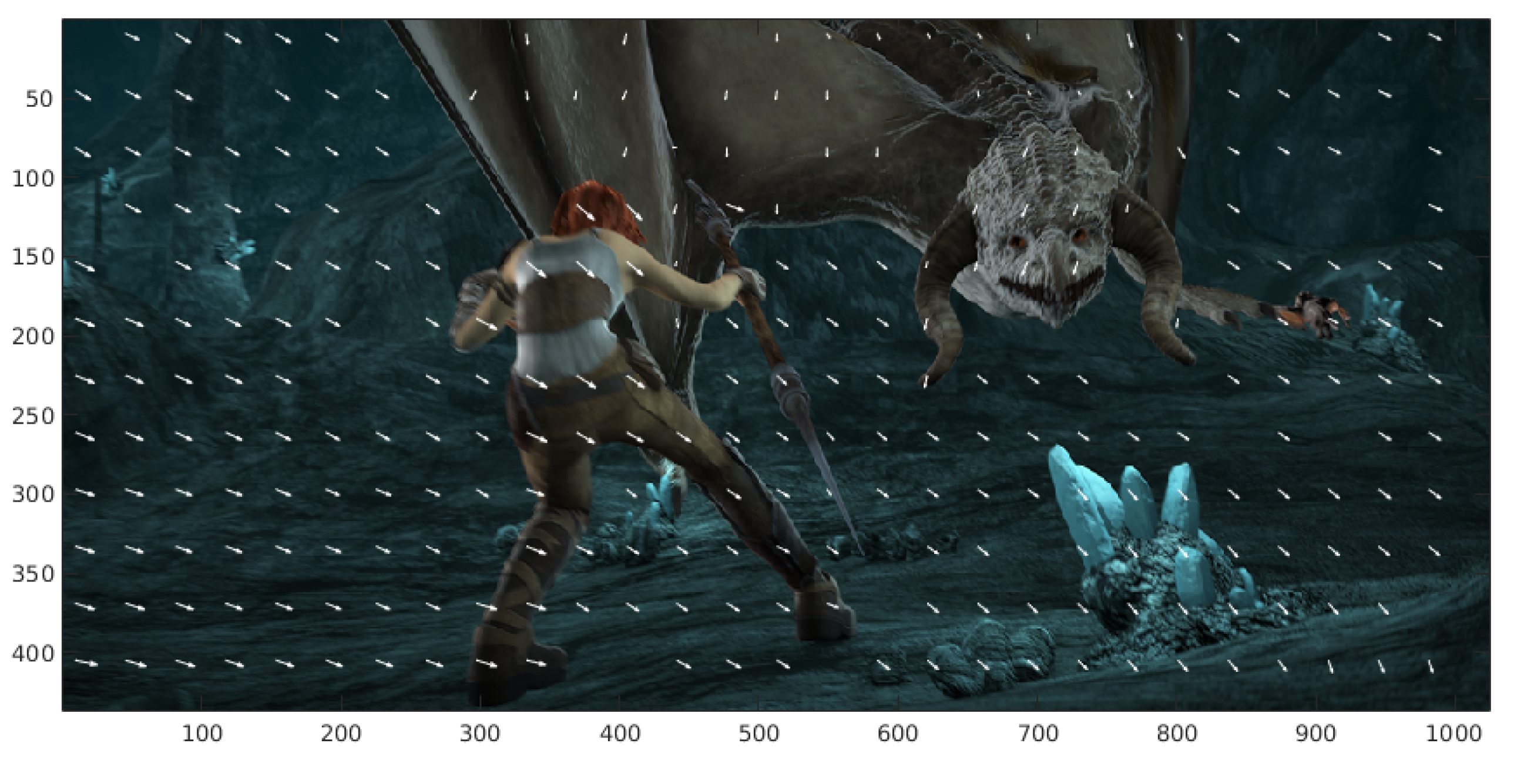
Figure 2.
Correspondences of patches located uniformly in the reference image.
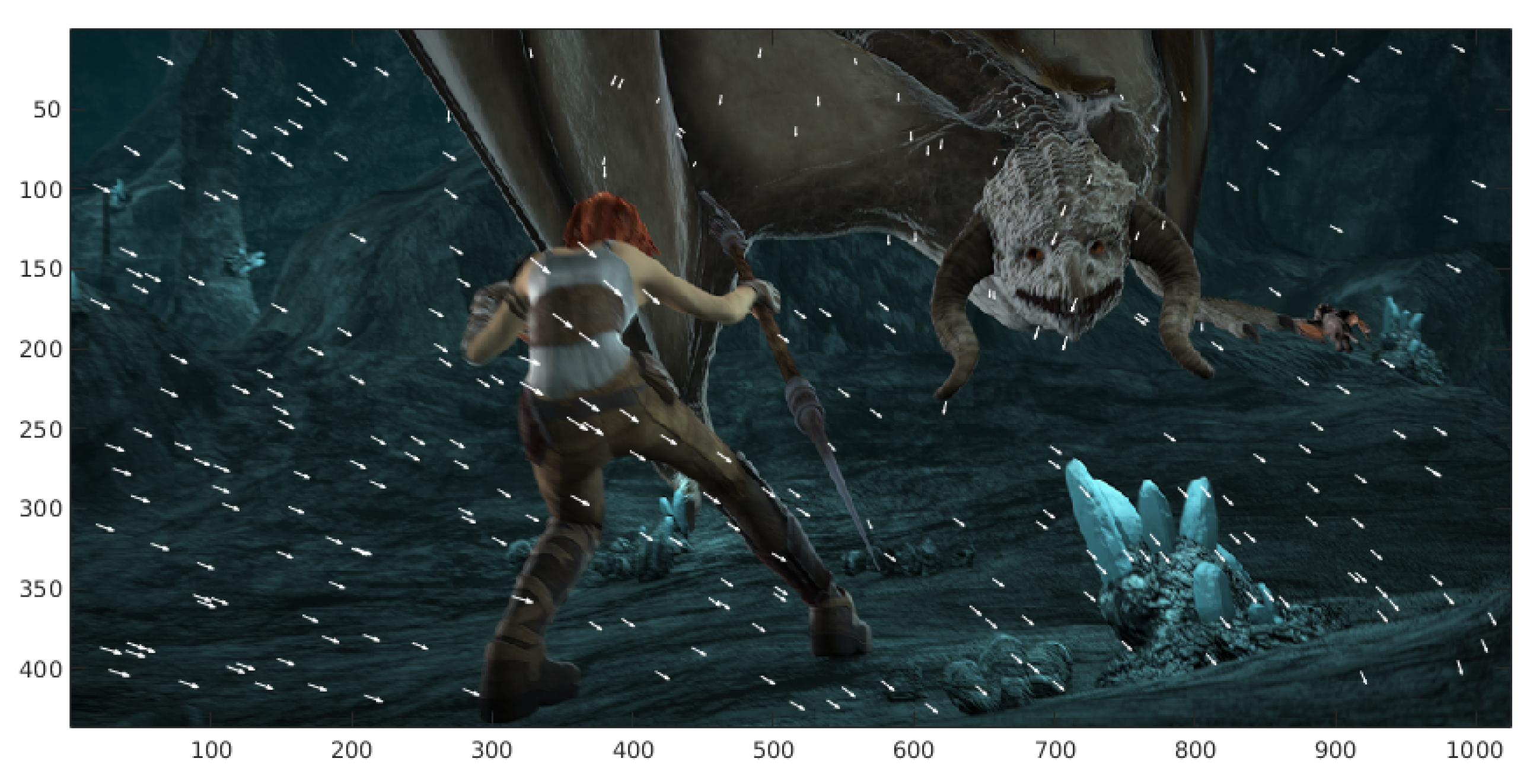
Figure 3.
Correspondences of patches located randomly in the reference image.
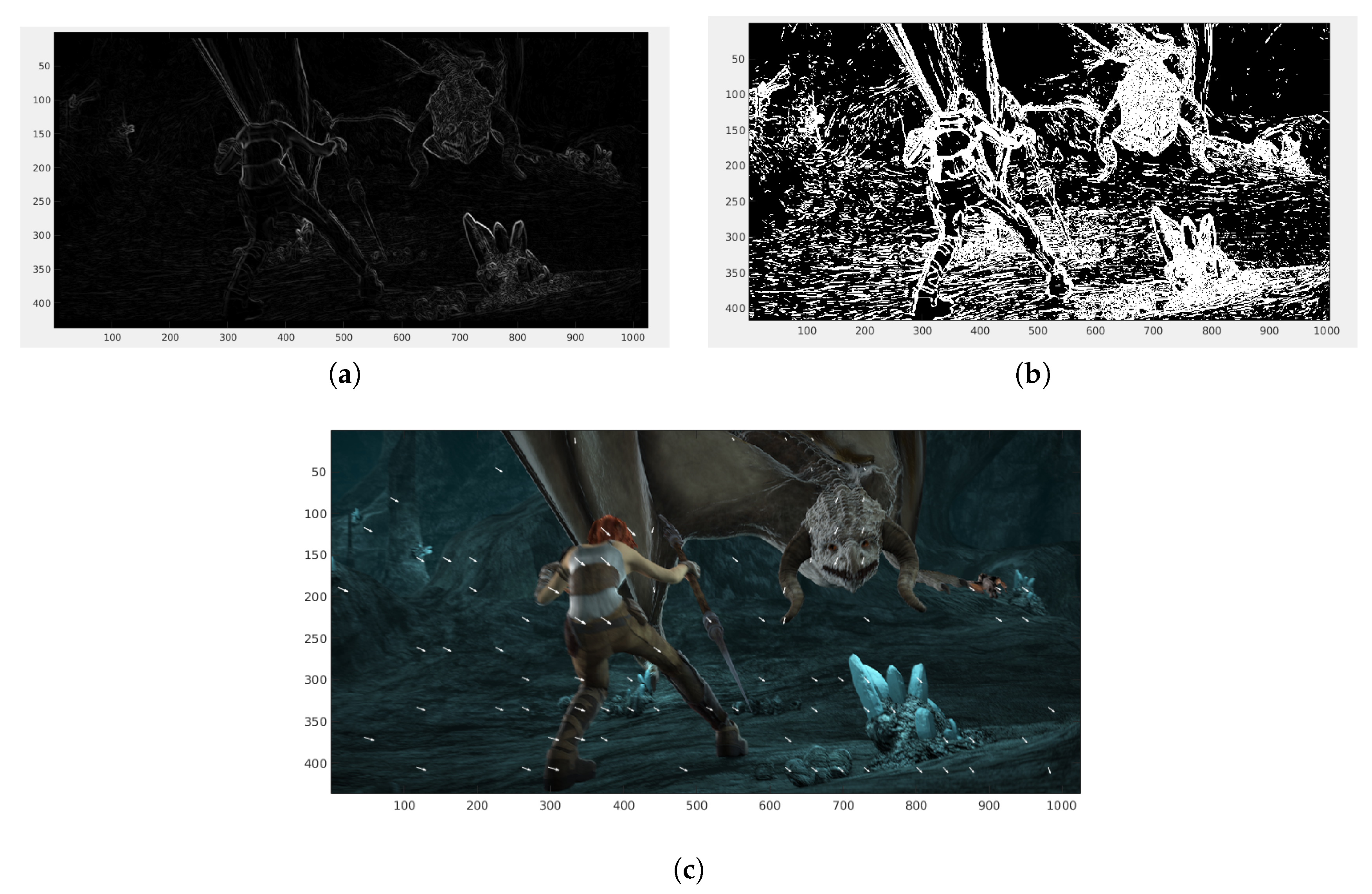
Figure 4.
Correspondence of patches located in the largest magnitude of the gradient. (a) Gradient magnitude of the reference image. (b) Ordered gradient from the minimum magnitude to the maximum magnitude. (c) Correspondences of the patches located in the maximum gradient magnitudes (white arrows).
Figure 5.
(a) Gradient of the reference image. (b) Large gradient set. (c) Matching result of patches located in the large gradient uniform grid.
Figure 6.
(a) Gradient of the reference image. (b) Medium gradient set. (c) Matching result of the patches located in the medium gradient uniform grid.
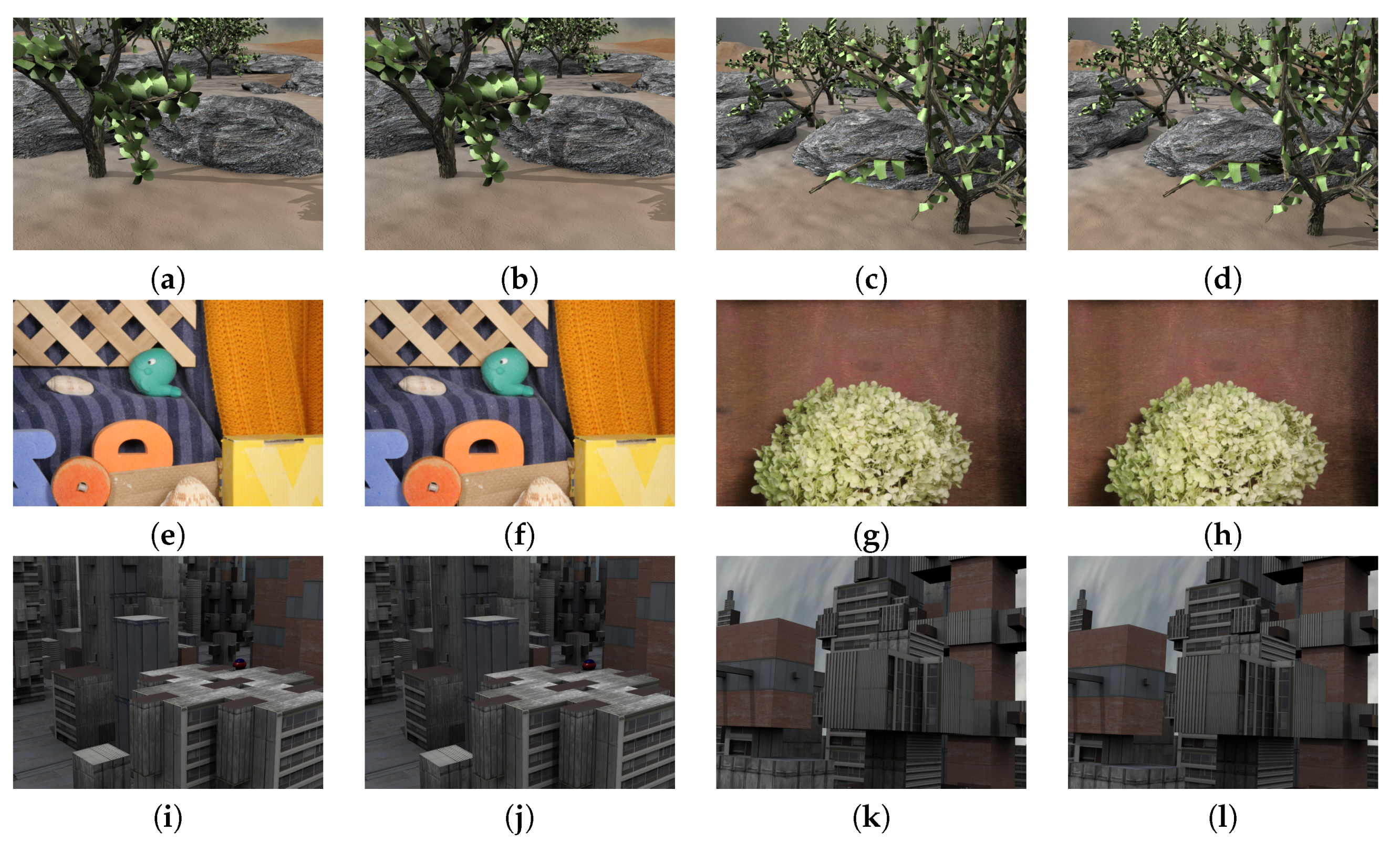
Figure 7.
Images of the Middlebury database containing small displacements. (a) and (b) frame10 and frame11 of sequence Grove2, respectively. (c) and (d) frame10 and frame11 of sequence Grove3, respectively. (e) and (f) frame10 and frame11 of sequence RubberWhale, respectively. (g) and (h) frame10 and frame11 of sequence Hydrangea, respectively. (i) and (j) frame10 and frame11 of sequence Urban2, respectively and finally (k) and (l) of sequence Urban2, respectively.
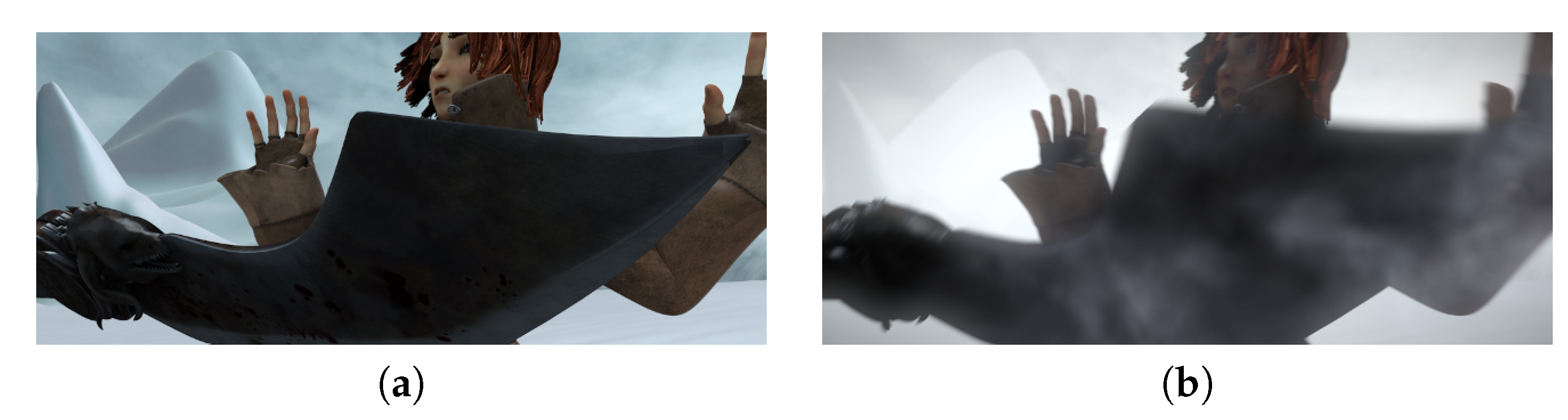
Figure 8.
Image extracted from MPI-Sintel clean version and MPI-Sintel final version. We extracted frame_0014 from sequence ambush_2. (a) frame_0014 clean version. (b) frame_0014 final version.
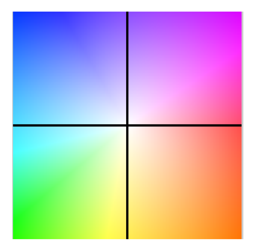
Figure 9.
Color code used for the optical flow.
Figure 10.
Examples of images of the MPI-Sintel database video sequence. (a,b) frame_0010 and frame_0011, (c) color-coded ground truth optical flow of the cave_4 sequence, (d) ground truth represented with arrows. (e,f) frame_0045 and frame_0046, (g) color-coded ground truth, and (h) arrow representation of optical flow of the cave_4 sequence, (i,j) frame_0030 and frame_0031, (k) color-coded ground truth optical flow, (l) arrow representation (in blue) of the temple3 sequence. (m,n) frame_0006 and frame_0007, (o) color-coded ground truth and (p) arrow representation (in green) ground truth optical flow of the ambush_4 sequence.
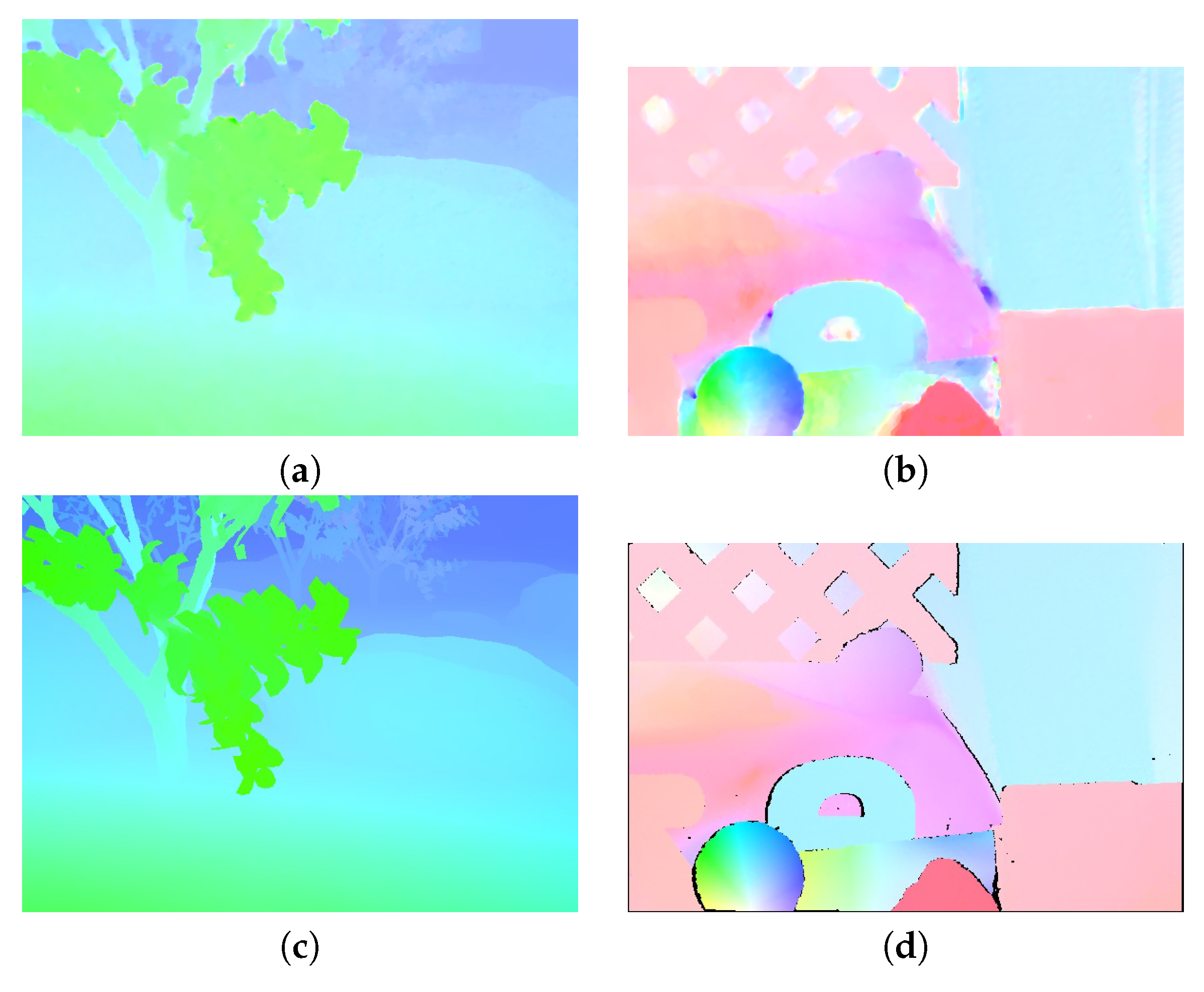
Figure 11.
Color-coded optical flow. (a) Color-coded optical flow for Grove2. (b) Color-coded optical flow for RubberWhale. (c) Ground truth for the Grove2 sequence. (d) Ground truth for the RubberWhale sequence.
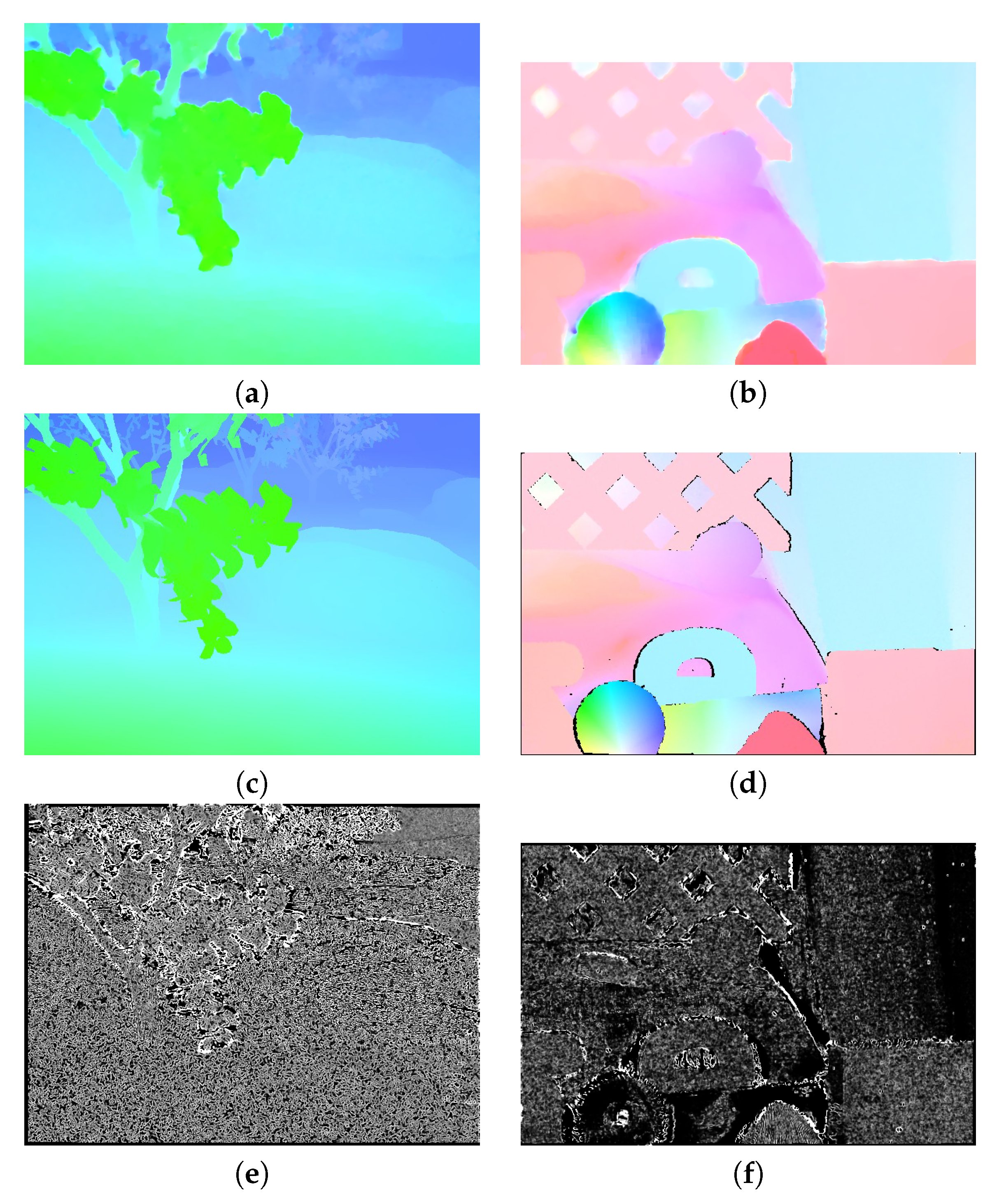
Figure 12.
Color-coded optical flow. (a) Color-coded coded optical flow for Grove2. (b) Color-coded optical flow for RubberWhale. (c) Ground truth for the Grove2 sequence. (d) Ground truth for the RubberWhale sequence. (e) Weight map for Grove2. (f) Weight map for RubberWhale.
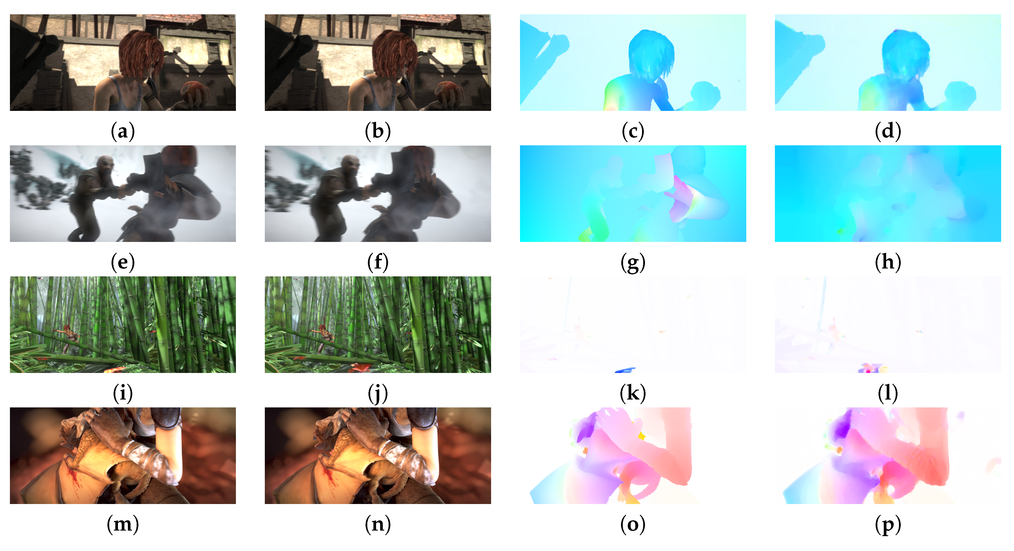
Figure 13.
Image sequences used to estimate model parameters. In the parameter estimation, we used the first two frames of each considered sequence: (a–d) the frames of the alley_1 sequence, the ground truth, and our results, respectively. (e,f) the ambush_2 sequence, (g) the ground truth, and (h) our result. (i,j) frames of the bamboo_2 sequence, (k) the ground truth, and (l) our result. (m,n) the frame of bandage_1 sequence (o) the ground truth, and (p) our results.
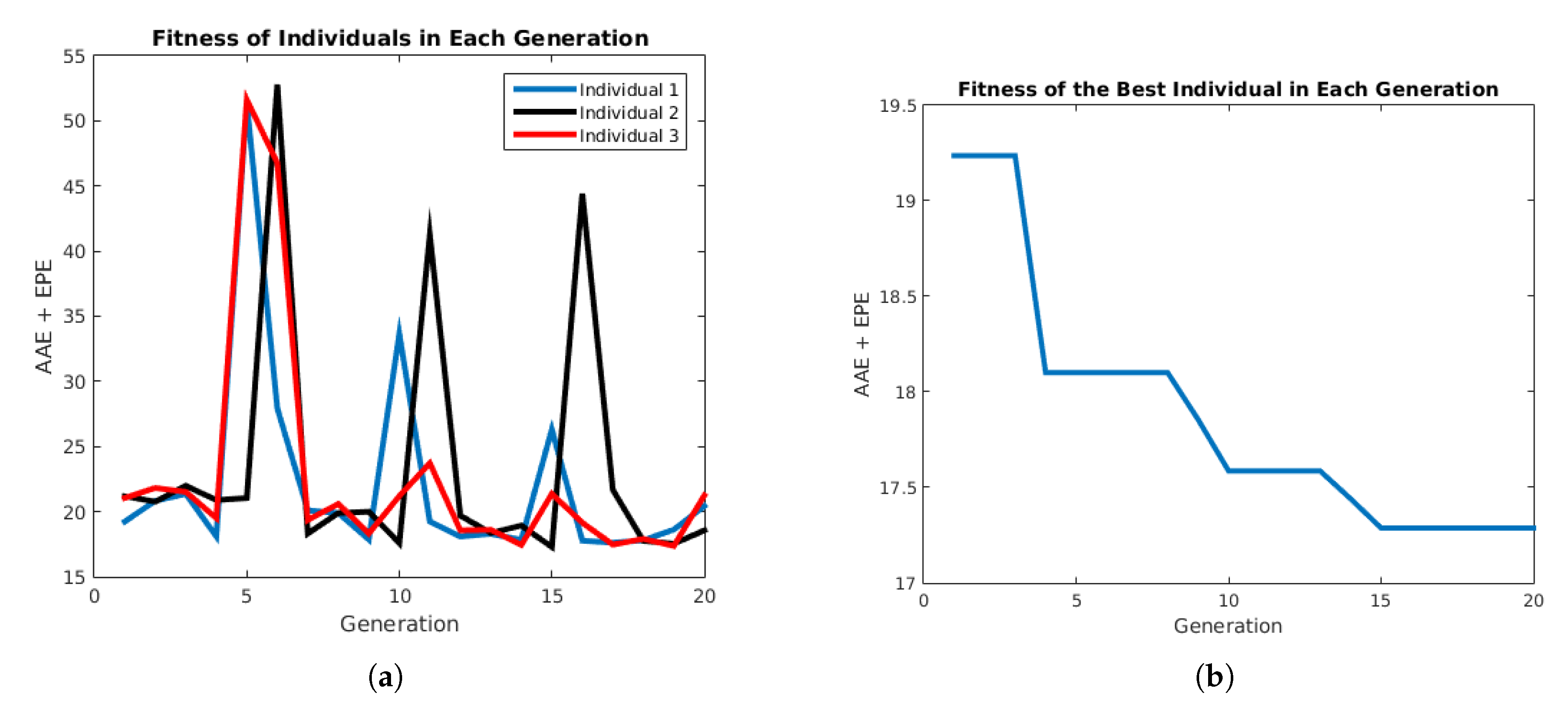
Figure 14.
Performance of the PSO algorithm. (a) Performance of each individual. (b) Performance of the best individual in each generation.
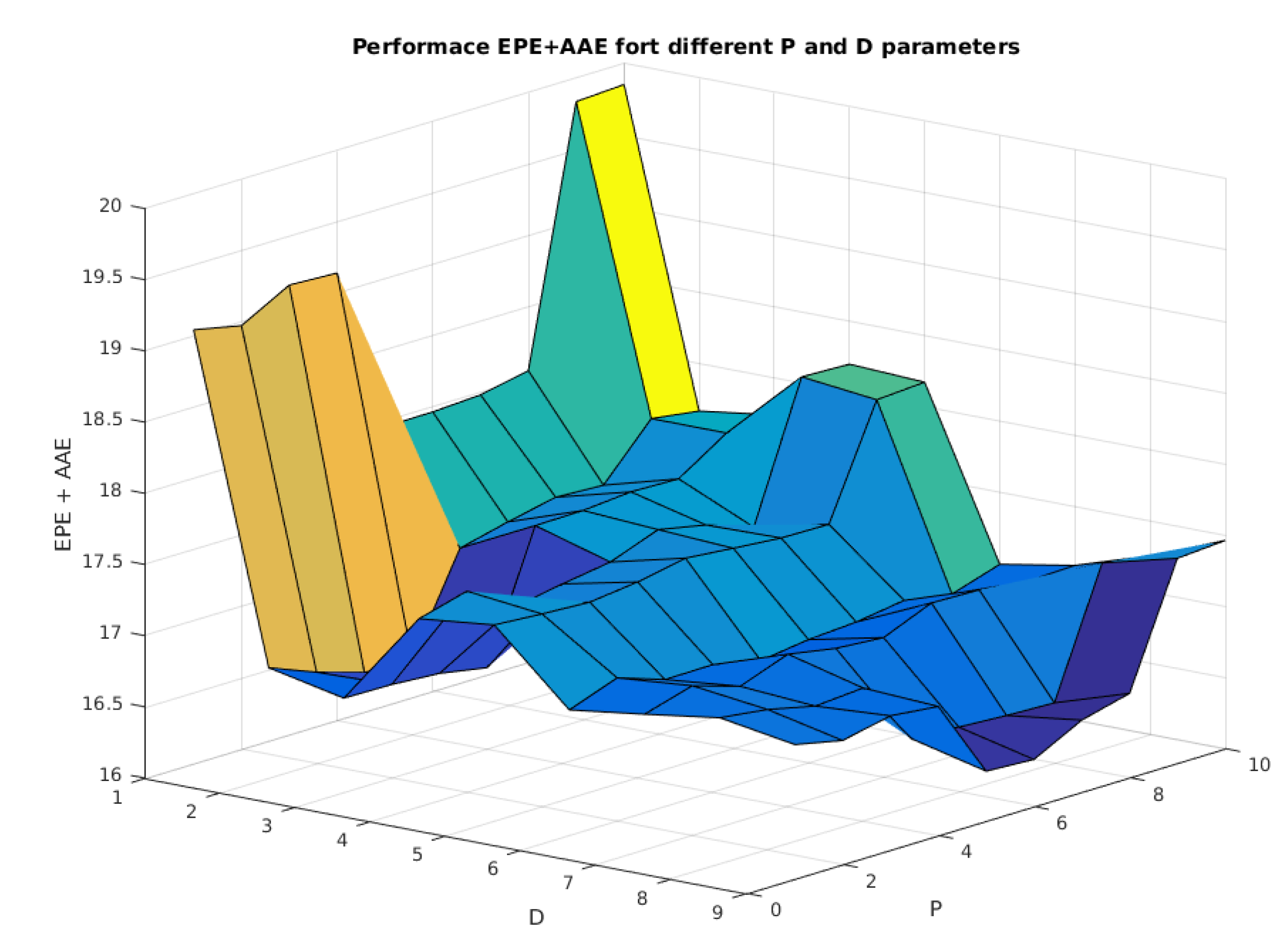
Figure 15.
Performance of the proposed model considering variation in P and D parameters.
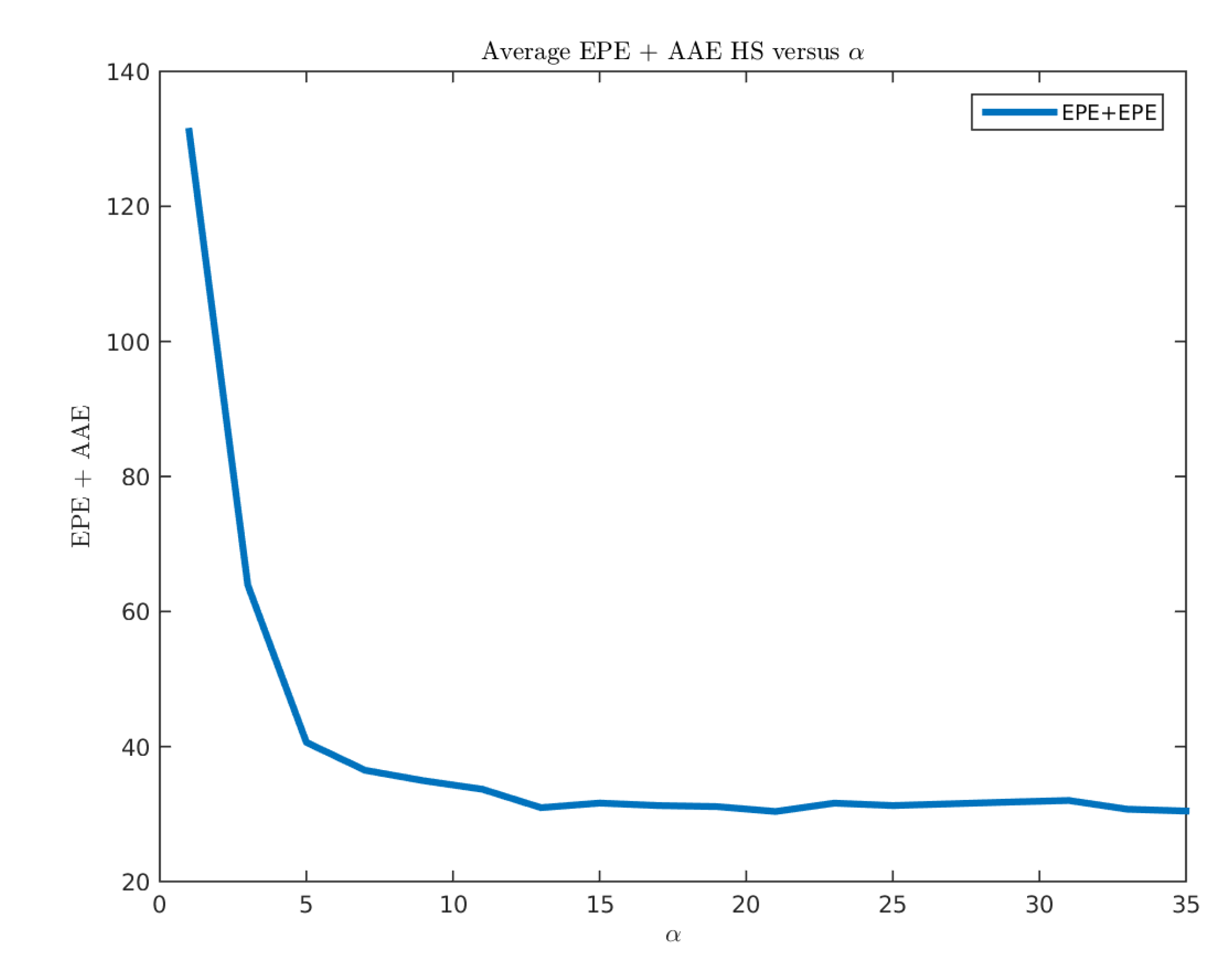
Figure 16.
Performance of the Horn-Schunck method for different values.
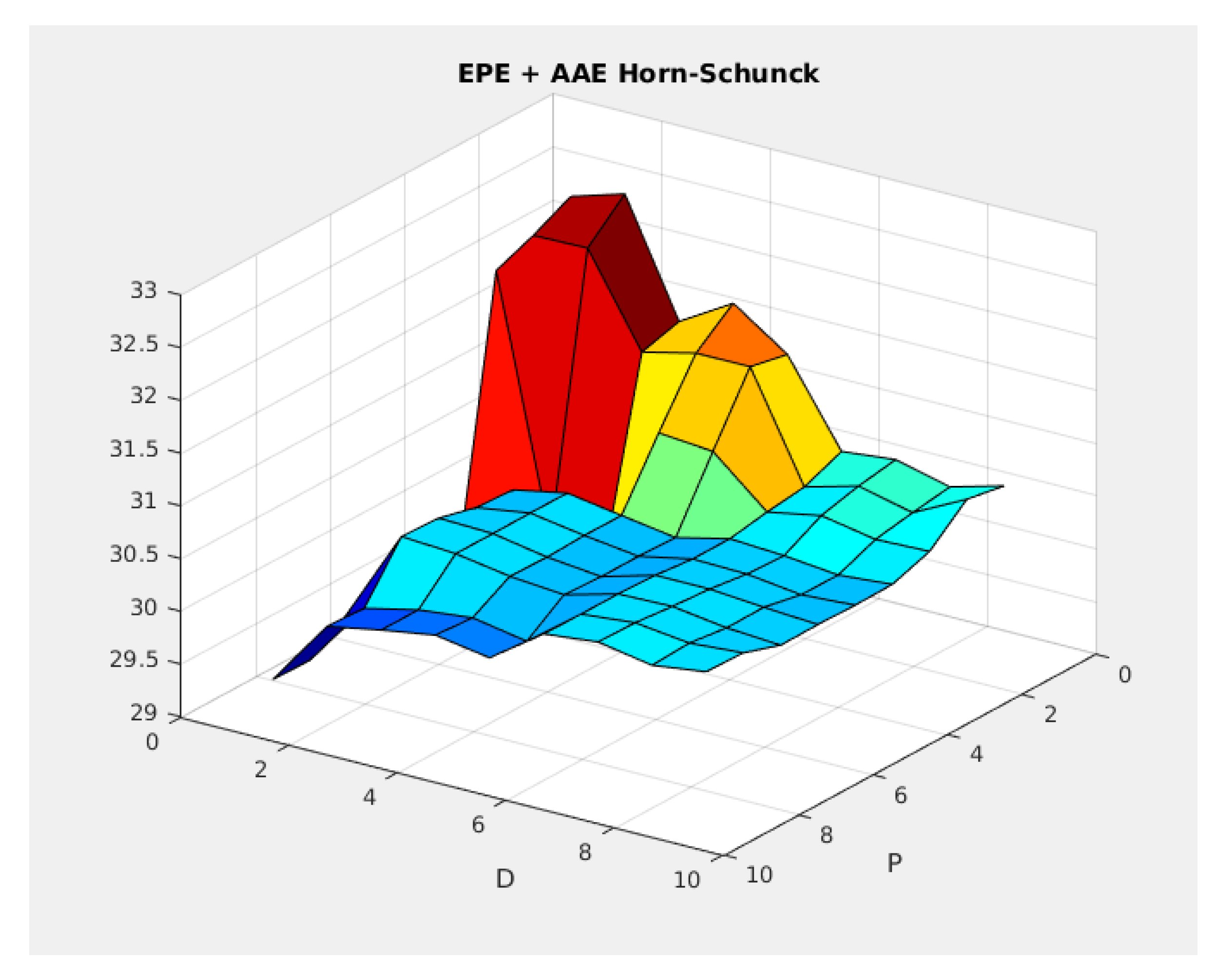
Figure 17.
Performance of the Horn-Schunck model for different P and D parameters.
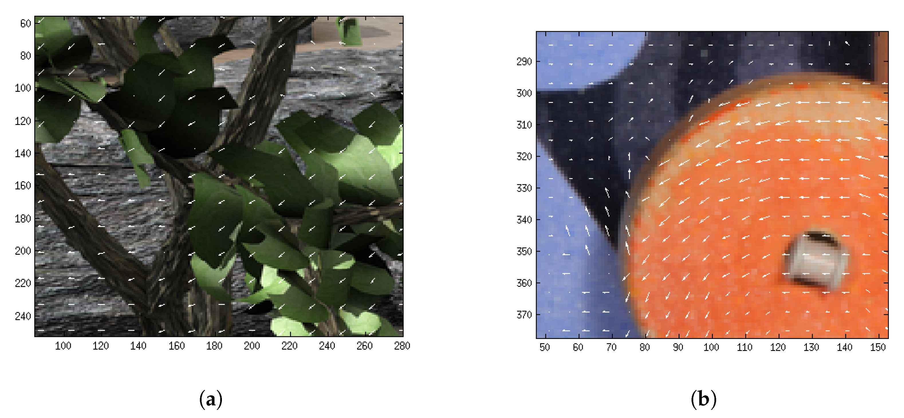
Figure 18.
Exhaustive matching represented with white arrows. (a) Exhaustive matching using and for Grove2. (b) Exhaustive matching using and for Rubberwhale.
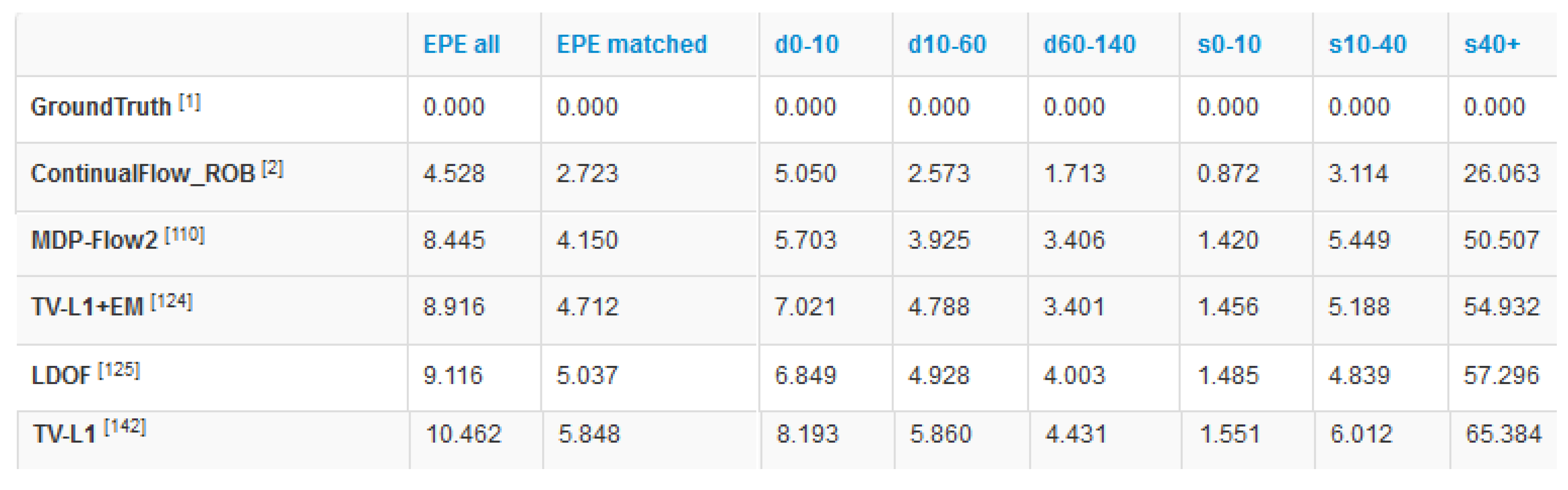
Figure 19.
Obtained results by our method in the MPI-Sintel test database (at 18 October 2018).
Table 1.
Number of images in each image sequence.
| Sequence Name | Number of Images |
|---|
| alley | 100 |
| ambush | 174 |
| bamboo | 100 |
| bandage | 100 |
| cave | 100 |
| market | 140 |
| mountain | 50 |
| shaman | 100 |
| sleeping | 100 |
| temple | 100 |
| Total images | 1064 |
Table 2.
PSO parameters.
| Parameter | Value |
|---|
| NIndividuals | 3 |
| NGeneration | 20 |
| NSequences | 8 |
| 0.5 |
| 0.5 |
| 1.0 |
Table 3.
Results obtained by PSO in the MPI-Sintel selected training set.
| | alley_1 | ambush_4 | bamboo_2 | bandage_1 | cave_4 | market_5 | mountain_1 | temple_3 |
|---|
| | | | | | | | |
| | | | | | | | |
Table 4.
Results obtained by PSO in the MPI-Sintel selected training set.
| | alley_1 | ambush_4 | bamboo_2 | bandage_1 | cave_4 | market_5 | mountain_1 | temple_3 |
|---|
| | | | | | | | |
| | | | | | | | |
Table 5.
Results obtained by the PSO in the MPI-Sintel selected training set.
| | alley_1 | ambush_4 | bamboo_2 | bandage_1 | cave_4 | market_5 | mountain_1 | temple_3 |
|---|
| | | | | | | | |
| | | | | | | | |
Table 6.
The reported performance of TV-L1 in Middlebury [
1].
| Error | Dime | Grove3 | Hydra | Urban3 | Venus | Average |
|---|
| 0.162 | 0.721 | 0.258 | 0.711 | 0.394 | 0.4492 |
| 2.888 | 6.590 | 2.814 | 6.631 | 6.831 | 5.1508 |
Table 7.
Obtained results of our model in Middlebury with .
| Error | Dime | Grove3 | Hydra | Urban3 | Venus | Average |
|---|
| 0.0925 | 0.7090 | 0.1729 | 0.7078 | 0.3492 | 0.4063 |
| 1.8248 | 6.5913 | 2.0626 | 6.9080 | 6.0818 | 4.6937 |
Table 8.
Results obtained by the uniform matching location strategy in VALIDATION_SET.
| Error | Dime | Grove3 | Hydra | Urban3 | Venus | Average |
|---|
| 0.0975 | 0.6924 | 0.1672 | 0.4811 | 0.3034 | 0.3485 |
| 1.8739 | 6.4759 | 2.0160 | 4.334 | 4.2259 | 3.7872 |
Table 9.
Average and obtained by Random Location Strategy in VALIDATION_SET set.
| Error | Dime | Grove3 | Hydra | Urban3 | Venus | Average |
|---|
| 0.0967 | 0.6798 | 0.1666 | 0.5446 | 0.2988 | 0.3573 |
| 1.8876 | 6.3781 | 2.0214 | 4.8060 | 4.1977 | 3.8581 |
Table 10.
Average and obtained by the maximum gradient location strategy in VALIDATION_SET.
| Error | Dime | Grove3 | Hydra | Urban3 | Venus | Average |
|---|
| 0.0938 | 0.7147 | 0.1772 | 0.7338 | 0.3014 | 0.4042 |
| 1.8596 | 6.5793 | 2.1159 | 5.9172 | 4.3285 | 4.1601 |
Table 11.
Summary of results. The end point error and average angular error obtained by uniform locations in the MPI-Sintel training set.
| Sequence Name | | |
|---|
| alley | 0.36 | 3.05 |
| ambush | 19.72 | 26.07 |
| bamboo | 1.68 | 13.66 |
| bandage | 0.64 | 7.01 |
| cave | 9.26 | 13.13 |
| market | 8.79 | 13.61 |
| mountain | 1.02 | 10.29 |
| shaman | 0.38 | 7.18 |
| sleeping | 0.11 | 1.79 |
| temple | 9.94 | 13.71 |
| Total | 5.58 | 10.87 |
| 16.45 | |
Table 12.
Summary of results. The end point error and average angular error obtained by random locations in the MPI-Sintel training set.
| Sequence Name | | |
|---|
| alley | 0.36 | 3.04 |
| ambush | 19.59 | 25.70 |
| bamboo | 1.69 | 13.69 |
| bandage | 0.64 | 7.02 |
| cave | 9.54 | 13.52 |
| market | 8.78 | 13.72 |
| mountain | 1.02 | 10.31 |
| shaman | 0.38 | 7.19 |
| sleeping | 0.11 | 1.79 |
| temple | 10.16 | 14.03 |
| Total | 5.62 | 10.91 |
| 16.53 | |
Table 13.
Summary of results. The end point error and average angular error obtained by locations on maximum gradients in the MPI-Sintel training set.
| Sequence Name | | |
|---|
| alley | 0.37 | 3.05 |
| ambush | 19.83 | 26.50 |
| bamboo | 1.66 | 13.56 |
| bandage | 0.65 | 7.04 |
| cave | 9.72 | 14.18 |
| market | 8.88 | 13.78 |
| mountain | 1.00 | 10.22 |
| shaman | 0.37 | 7.12 |
| sleeping | 0.11 | 1.79 |
| temple | 9.90 | 14.46 |
| Total | 5.64 | 11.10 |
| 16.73 | |
Table 14.
Summary of the obtained results for different strategies.
| Strategy | | |
|---|
| Uniform | 5.58 | 10.87 |
| Random | 5.62 | 10.91 |
| Maximum Gradient | 5.64 | 11.10 |
Table 15.
Summary of results. The end point error and average angular error obtained by the combination of uniform and large gradients in the MPI-Sintel training set.
| Sequence Name | | |
|---|
| alley | 0.36 | 3.03 |
| ambush | 19.85 | 26.43 |
| bamboo | 1.70 | 13.60 |
| bandage | 0.65 | 7.03 |
| cave | 9.84 | 14.39 |
| market | 9.10 | 14.07 |
| mountain | 0.98 | 10.24 |
| shaman | 0.38 | 7.16 |
| sleeping | 0.11 | 1.78 |
| temple | 10.03 | 14.31 |
| Total | 5.70 | 11.14 |
| 16.83 | |
Table 16.
Summary of results. The end point error and average angular error obtained by the combination of uniform and medium gradients in the MPI-Sintel training set.
| Sequence Name | | |
|---|
| alley | 0.63 | 5.99 |
| ambush | 26.42 | 34.81 |
| bamboo | 3.16 | 27.47 |
| bandage | 1.19 | 18.21 |
| cave | 12.49 | 19.18 |
| market | 10.76 | 19.90 |
| mountain | 1.43 | 13.57 |
| shaman | 0.67 | 14.39 |
| sleeping | 0.14 | 2.44 |
| temple | 16.21 | 26.23 |
| Total | 5.67 | 11.10 |
| 16.77 | |
Table 17.
Summary of results. The end point error and average angular error obtained by Horn-Schunck in the MPI-Sintel training set.
| Sequence Name | | |
|---|
| alley | 0.36 | 3.02 |
| ambush | 19.91 | 26.46 |
| bamboo | 1.67 | 13.59 |
| bandage | 0.65 | 7.03 |
| cave | 9.77 | 14.32 |
| market | 9.10 | 14.07 |
| mountain | 0.99 | 10.24 |
| shaman | 0.38 | 7.16 |
| sleeping | 0.11 | 1.79 |
| temple | 9.80 | 13.90 |
| Total | 7.76 | 17.74 |
| 25.50 | |
Table 18.
Summary of results. The end point error and average angular error obtained by Horn-Schunck using uniform locations in the MPI-Sintel training set.
| Sequence Name | | |
|---|
| alley | 0.64 | 6.07 |
| ambush | 26.01 | 34.88 |
| bamboo | 3.52 | 28.04 |
| bandage | 1.19 | 18.14 |
| cave | 34.44 | 45.41 |
| market | 11.74 | 20.60 |
| mountain | 1.59 | 14.33 |
| shaman | 0.66 | 11.85 |
| sleeping | 0.29 | 2.95 |
| temple | 17.33 | 27.95 |
| Total | 10.16 | 20.95 |
| 30.76 | |


