Article

Hierarchical Data Decision Aided 2-Source BPSK H-MAC Channel Phase Estimator with Feed-Back Gradient Solver for WPNC Networks and Its Equivalent Model †

Department of Radio Engineering, Czech Technical University in Prague, 166 27 Praha 6, Czech Republic
This paper is an extended version of our paper published in WiMob2018: Sykora J. Hierarchical Data Decision Aided 2-Source BPSK H-MAC Channel Phase Estimator with Feed-Back Gradient Solver for WPNC Networks. In Proceedings of the 14th International Conference on Wireless and Mobile Computing, Networking and Communications (WiMob), Limassol, Cyprus, 15 October 2018; pp. 89–96.
Information 2019, 10(2), 40; https://doi.org/10.3390/info10020040
Submission received: 30 December 2018 / Revised: 13 January 2019 / Accepted: 18 January 2019 / Published: 24 January 2019
(This article belongs to the Section Information and Communications Technology)

Abstract

:
This paper focuses on the channel state estimation (CSE) problem in parametrized Hierarchical MAC (H-MAC) stage in Wireless Physical Layer Network Coding (WPNC) networks with Hierarchical Decode and Forward (HDF) relay strategy. We derive a non-pilot based H-MAC channel phase estimator for 2 BPSK alphabet sources. The CSE is aided only by the knowledge of H-data decisions. At HDF relay, there is no information on individual source symbols available. The estimator is obtained by a marginalization over the hierarchical dispersion. The estimator uses a gradient additive update solver and the indicator function (gradient) is derived in exact closed form and in approximations for low and high SNR. We analyze the properties of the equivalent solver model, particularly the equivalent gradient detector characteristics and its main stable domain properties, and also the detector gain and equivalent noise properties under a variety of channel parameterization scenarios.

1. Introduction

1.1. Background and Context

Wireless Physical Layer Network Coding (WPNC) is a PHY layer concept for communications in dense radio networks with highly interacting signals. We have reached a relatively solid understanding of some fundamental limits and the system design and performance analysis in basic topologies and scenarios [1,2,3,4,5]. This includes knowledge of achievable and converse rates for specific strategies and scenarios (e.g., Compute & Forward, Noisy Network Coding, Hierarchical Decode and Forward (HDF)), design of Network Coded Modulation (NCM) and related hierarchical demodulation and decoding strategies including their performance analysis. Most of the results assume relatively idealized assumptions related to relative channel parametrization and NCM codebooks used at source nodes.
This paper focuses on the channel state estimation (CSE) problem in parametrized Hierarchical MAC (H-MAC) stage (A prefix ‘H-’ denotes hierarchical entities, i.e., many-to-one functions of source node entities (see [1] for details)). The H-decoding and H-demodulation performance in H-MAC depends strongly on the knowledge of the channel parametrization. This holds generally for all communications systems. However, in the case of WPNC, particularly with HDF strategy, the relative (among all source nodes) channel parametrization becomes of paramount importance, since (apart of significant performance consequences) it affects the overall structure of the hierarchical (soft-output) demodulator (H-SODEM). Namely, it affects the shape of H-constellation which is a highly complicated nonlinear function of the relative fading. This problem becomes even more significant in the randomly time-variant fading channels, where traditional pilot based approaches have limited applicability. We develop a non-pilot based H-MAC channel state estimator which provides good tracking performance in time-variant environments. Due to the paper length restriction, we constrain the exposition of background WPNC theory and terminology/notation at the minimum necessary level needed for the contribution of the paper. Thorough additional details can be found in [1].

1.2. Goals and Contributions

For classical single user (orthogonally separated) communications, the pilot based CSE is a widely adopted and relatively easily implementable concept. In the WPNC networks, it has however a limited applicability. In order to obtain acceptable accuracy of the estimates (see e.g., Cramer-Rao lower bound analysis in [1]), the pilots from individual sources must be orthogonal. This is however a strong contradiction of the whole WPNC concept which uses mutually interacting non-orthogonal signals. Orthogonal resources can be created only be time-division—letting only one source be active at a given time. In a randomly time-varying channel environment, this would dramatically decrease the duty rate of data payload and thus the overall efficiency of the system. Moreover, the H-decoding in H-MAC is quite critically dependent on the CSE quality, particularly for the relative phase. Under these conditions, the CSE performed directly on the random data payload stream is a viable solution. Apart from avoiding, or minimizing the need for pilots (possibly only used for the ambiguity resolution), it also opens a natural way for CSE algorithms to continuously track the time-varying H-MAC channel.
The H-MAC CSE in the WPNC networks is significantly different from the classical CSE cases. Most importantly, we estimate the channel parameters of several nonorthogonal signals received in superposition. This makes the problem a multidimensional composite estimation problem of several channel parameters over a random payload data stream. There are several options for approaching this problem, ranging form non-data aided (where we marginalize the observation likelihood over a priori data statistic), through various data soft-information aided forms, to decision aided forms (where the decisions are provided from the decoder).
The data decision aided strategies have one specific problem in WPNC networks. The core principle underlying the whole treatment (otherwise, it would be quite straightforward) is the fact that we do not have available individual component source symbols s A , s B (nor messages b A , b B ) decisions available at the relay. This is a fundamental principle of HDF strategy. The whole system is operated from the information-theoretic point of view at the operational point where we do not have a chance to have reliable decoded individual component messages b A , b B (and consequently all c A , c B , and s A , s B ) but only their many-to-one HNC map c = χ c ( c A , c B ) which is called H-data (or H-symbols).
The CSE may be thus aided only by H-data information. Due to the many-to-one HNC map property, there is still a randomness in the payload data even for fixed given H-data knowledge. This is called H-dispersion and CSE will have to marginalize it from its utility function.

1.3. Related Work

The problem of CSE in WPNC H-MAC channel is somewhat similar to CSE in MISO or MIMO systems, where the signals from different transmit antennas also interact on the given receive antenna. However, the applicability of those methods (see e.g., [6] and the references therein) for our case is limited since they are typically pilot based and rely on some form of the orthogonality of pilots from individual transmit antennas. The solution presented in our paper is non-pilot based. To the best of our knowledge, we are not aware of any other related work on WPNC CSE that would not require pilots and would work over the random data stream. All previous works essentially assume some form of orthogonal pilots (in many forms, e.g., for OFDM based waveforms). This fact also creates some problems for a performance comparison. Any pilot based system would have an “unfair” advantage (even while keeping the same power budget) over the non-pilot based CSE and thus any direct comparison would be difficult to interpret. We would have to take into account the additional resources needed for pilots that would reduce the payload resources for WPNC data. Since this would require also defining the payload coding and processing, it is outside the scope of this paper.

2. System Model

We consider a 2-component (2 source nodes SA, SB, one relay) H-MAC topology (Figure 1) with isomorphic layered NCM and symbol-timing synchronized nodes. Component messages are b A , b B and the target on the relay is to decode a hierarchical message b = χ ( b A , b B ) which is a many-to-one function (Hierarchical Network Code (HNC) map) of the source messages. We consider only the processing on one relay and assume that the end-to-end solvability is fulfilled by a proper choice of all remaining components of WPNC network (see [1] for end-to-end solvability conditions). The component messages are encoded by a common codebook C , c A = C ( b A ) , c B = C ( b B ) . The coded symbols are symbol-wise mapped on the channel constellation points s A , n = A s ( c A , n ) , s B , n = A s ( c B , n ) . A s is the source 1-dimensional constellation alphabet with size M s .
The isomorphic property of NCM guarantees that H-code symbols c = C ( b ) are HNC maps of component coded symbols c n = χ c ( c A , n , c B , n ) . In this paper, we consider minimal HNC map χ c , i.e., such that given the knowledge of H-symbol c n and any of component symbols c A , n (or c B , n ), we can uniquely determine the other source symbol c B , n (or c A , n ).
The H-MAC memory-less AWGN channel is modeled as
x = h A s A ( c A ) + h B s B ( c B ) + w
where h A = η A e j φ A , h B = η A e j φ B are fading coefficients and w is AWGN vector with σ w 2 variance per dimension. The observation vector has length N. Signal to noise ratio (SNR) is defined w.r.t. source A signal and it is γ x = E [ | s A | 2 ] / σ w 2 .
Since the channel is memory-less, the noise is white, and the constellation mappers are symbol-wise, the complete frame observation likelihood is p ( x | φ A , φ B , c A , c B ) = n p ( x | φ A , φ B , c A , n , c B , n ) . The symbol-wise likelihood is (For a notational simplicity (unless it is explicitly needed), we drop the explicit sequential index n notation, e.g., x x n , and similarly others.)
p ( x | φ A , φ B , c A , c B ) e 1 σ w 2 x η A e j φ A s A ( c A ) η B e j φ B s B ( c B ) 2
where we dropped unimportant scaling in the Gaussian density. Channel coefficient magnitudes η A , η B R + are assumed to be known at the relay.
In this paper, we focus on a special case of both sources having BPSK alphabets A s = { ± 1 } , i.e., s A ( c A ) = 2 c A 1 , c A { 0 , 1 } , and similarly for s B . In the case of binary symbol-wise HNC map, the only possible choice fulfilling the minimal cardinality condition is the XOR map c = c A c B , c { 0 , 1 } .

3. H-Data Decision Aided H-MAC CSE

We derive the H-data decision aided ML (Maximum Likelihood) CSE for 2-source BPSK H-MAC. The estimator does not have available the individual messages b A , b B (nor c A , c B , and s A , s B ) but only their many-to-one HNC map c = χ c ( c A , c B ) . This is provided by the H-decoder (Figure 1), and we assume that the estimates are reliable c ^ = c . The random hierarchical dispersion [1] remains unknown. It must be marginalized from the observation likelihood. Under special conditions (namely the minimal HNC map), we will be able to model its stochastic properties needed for the marginalization.

3.1. H-Dispersion Marginalization for 2-Source BPSK

First, we perform a simple manipulation with symbol-wise observation likelihood. We use the fact that the source constellation mappers s A ( c A ) , s B ( c B ) are one-to-one functions, and both of them are from the PSK class of alphabets | s A | = | s B | = 1
p ( x | φ A , φ B , s A , s B ) exp 2 σ w 2 η A η B e j ( φ A φ B ) s A s B × exp 2 σ w 2 η A x e j φ A s A + η B x e j φ B s B .
We dropped all scaling which do not depend on φ A , φ B , s A , s B .
The marginalization of the H-dispersion means a marginalization over all source symbols consistent with H-symbol, i.e., ( s A , s B ) : c f ( s A , s B ) where f ( ) is the marginalized entity. The minimal HNC map defines a unique value of s B for a given pair of s A , c . For the 2-source BPSK NCM with XOR map, it is
s B = s B c B ( c , c A ) = s B ( c c A ) = ( 1 2 c ) s A .
Then the H-dispersion marginalization can be evaluated as
p ( x | φ A , φ B , c ) = 1 p ( c ) ( s A , s B ) : c p ( x | φ A , φ B , s A , s B ) p ( s A ) p ( s B ) = 1 p ( c ) s A p x | φ A , φ B , s A , s B ( s A , c ) p ( s A ) p ( s B ) .
The minimal map together with IID source symbols guarantee [1] that p ( s A ) = p ( s B ) = p ( c ) = 1 / M s .
We define cross inner product symbol s = s A s B and a class of NCM called H-symbol inner product unique ones, that fulfill the property that the inner product symbol s is uniquely defined by the H-symbol c, i.e., s ( c ) is one-to-one function. The 2-source BPSK NCM with XOR map fulfills that and it holds
s ( c ) = s A s B = ( 1 2 c ) s A 2 = 1 2 c .
We also see that for any PSK alphabet s B = s ( c ) s A .
The marginalized H-symbol conditioned channel phases likelihood is then (dropping all unimportant scaling)
p ( x | φ A , φ B , c ) s A { ± 1 } exp 2 σ w 2 η A η B e j ( φ A φ B ) s ( c ) × exp 2 σ w 2 η A x e j φ A s A + η B x e j φ B s ( c ) s A = exp 2 σ w 2 η A η B s ( c ) cos ( φ A φ B ) × 2 cosh 2 σ w 2 η A x e j φ A + η B s ( c ) x e j φ B .
The phase estimator metric ρ is defined as a logarithm of scaled (dropping all unimportant scaling) p ( x | φ A , φ B , c ) , i.e.,
ρ = 2 σ w 2 η A η B s ( c ) cos ( φ A φ B ) + ln cosh 2 σ w 2 η A x e j φ A + η B s ( c ) x e j φ B .
For the whole observation frame, we have ρ N ( φ A , φ B , c ) = n = 1 N ρ ( φ A , φ B , c n ) .
The ML CSE is then
φ ^ = [ φ ^ A , φ ^ B ] = arg min φ A , φ B ρ N ( φ A , φ B , c )
for H-symbols c provided by the H-decoder.

3.2. Feed-Back Gradient Solver

Clearly, a direct solution of ML CSE is unfeasible. We need to resort to the feed-back iterative solver based on the gradient based additive updates. At i-th iteration, the estimate update is
φ ^ ( i + 1 ) = φ ^ ( i ) + K φ ρ N ( φ ^ ( i ) , c )
where K is the loop gain. The gradient indicator has symbol-wise components μ A = ρ / φ A and μ B = ρ / φ B , μ = [ μ A , μ B ] . The complete frame observation gradient is μ N = φ ρ N ( φ ^ ( i ) , c ) = n μ ( φ ^ ( i ) , c n ) .
Performing the derivatives, we get
μ A = 2 σ w 2 η A η B s ( c ) sin ( φ A φ B ) + 2 σ w 2 η A x e j φ A × tanh 2 σ w 2 η A x e j φ A + η B s ( c ) x e j φ B ,
μ B = 2 σ w 2 η A η B s ( c ) sin ( φ B φ A ) + 2 σ w 2 η B x e j φ B × tanh 2 σ w 2 η B x e j φ B + η A s ( c ) x e j φ A .
The expressions are, as expected, symmetric w.r.t. φ A and φ B , and are the exact expressions including a proper scaling (needed e.g., for Cramer-Rao lower bound analysis).
A practical implementation of these expressions calls for approximations avoiding complicated nonlinear functions. In the next, we determine an approximation for low and high SNR. The low and high SNR scenarios are defined in terms of the power ratio of the direct signals from source A and B to AWGN noise variance. The H-MAC channel also has an additional degree of freedom given by a ratio of signal powers from A and B. For our analysis, we consider these powers to be roughly similar (practically about ± 10 dB). A very good justification for this assumption comes from the very basic nature of WPNC systems. They demonstrate their main throughput performance advantages (against classical systems) in the interference limited region [1] and thus these systems are mainly used in such scenarios. Any conditions regarding low/high SNR thus apply to both links.
For low SNR scenarios, we can assume that η A 2 / σ w 2 and η B 2 / σ w 2 are very small, and thus η A x / σ w 2 ≪ 1 and η B x / σ w 2 ≪ 1. Then we can use the approximation tanh ( A ) A . The low SNR gradient indicator approximation is then (after some manipulations)
μ A 0 = 2 σ w 4 η A η B s ( c ) sin ( φ A φ B ) σ w 2 | x | 2 + 2 σ w 4 η A 2 x 2 e j 2 φ A + 2 σ w 4 η A η B s ( c ) x 2 e j ( φ A + φ B ) ,
μ B 0 = 2 σ w 4 η A η B s ( c ) sin ( φ B φ A ) σ w 2 | x | 2 + 2 σ w 4 η B 2 x 2 e j 2 φ B + 2 σ w 4 η A η B s ( c ) x 2 e j ( φ A + φ B ) .
For high SNR scenarios, we can assume that η A 2 / σ w 2 and η B 2 / σ w 2 are large, and thus η A x / σ w 2 1 and η B x / σ w 2 1 . Then we can use the approximation tanh ( A ) sign ( A ) . The high SNR gradient indicator approximation is then
μ A = 2 σ w 2 η A η B s ( c ) sin ( φ A φ B ) + 2 σ w 2 η A x e j φ A × sign η A x e j φ A + η B s ( c ) x e j φ B ,
μ B = 2 σ w 2 η A η B s ( c ) sin ( φ B φ A ) + 2 σ w 2 η B x e j φ B × sign η B x e j φ B + η A s ( c ) x e j φ A .

4. Equivalent Model of Feed-Back Solver

The performance analysis of the feed-back iterative solver with additive updates operating under time-variant channel parameter conditions and under random noise excitation is a complicated task, namely due to a combination of two phenomena—the nonlinearity and the random excitation. In our case, it is even more complex due to the multidimensional tracked entity ( φ A , φ B ). The analysis of the dynamic nonlinear state-space systems with random excitation is, on its own, an extremely wide field and exposing all details is completely out of the scope of this paper (see e.g., [7,8,9]).
Usually, the analysis is approached by forming an equivalent model. The equivalent model is formed in such a way that the variables of interest, typically the tracking error Δ φ = φ ^ φ , are directly processed as open state variables. This is in contrast with the true system, where these variables may be buried deeply inside the complex nonlinear functions. In addition, the equivalent model tries to separate the nonlinearity and the memory of the system and also considers only additive random excitation. Of course, with the exception of some very specific scenarios, this all makes the equivalent model just an approximation. However, the approximation is mathematically tractable by solving stochastic differential equations using Fokker-Planck equation.
The equivalent model approximates the true solver in terms of conditional first and second order moment equivalence (see e.g., [9,10]). The true indicator output μ is approximated by
μ e = K g g ( φ , φ ^ ) + ξ
where g is the equivalent detector characteristics, ξ = [ ξ A , ξ B ] T is the equivalent noise, and K g = diag ( K g A , K g B ) is a diagonal detector gain normalization matrix. The normalization is usually set to make the component gradients equal to unity at the main stable lock point, i.e., at Δ φ = 0 . This makes the detector gain easily interpretable as a part of the loop gain in the vicinity of stable lock point.

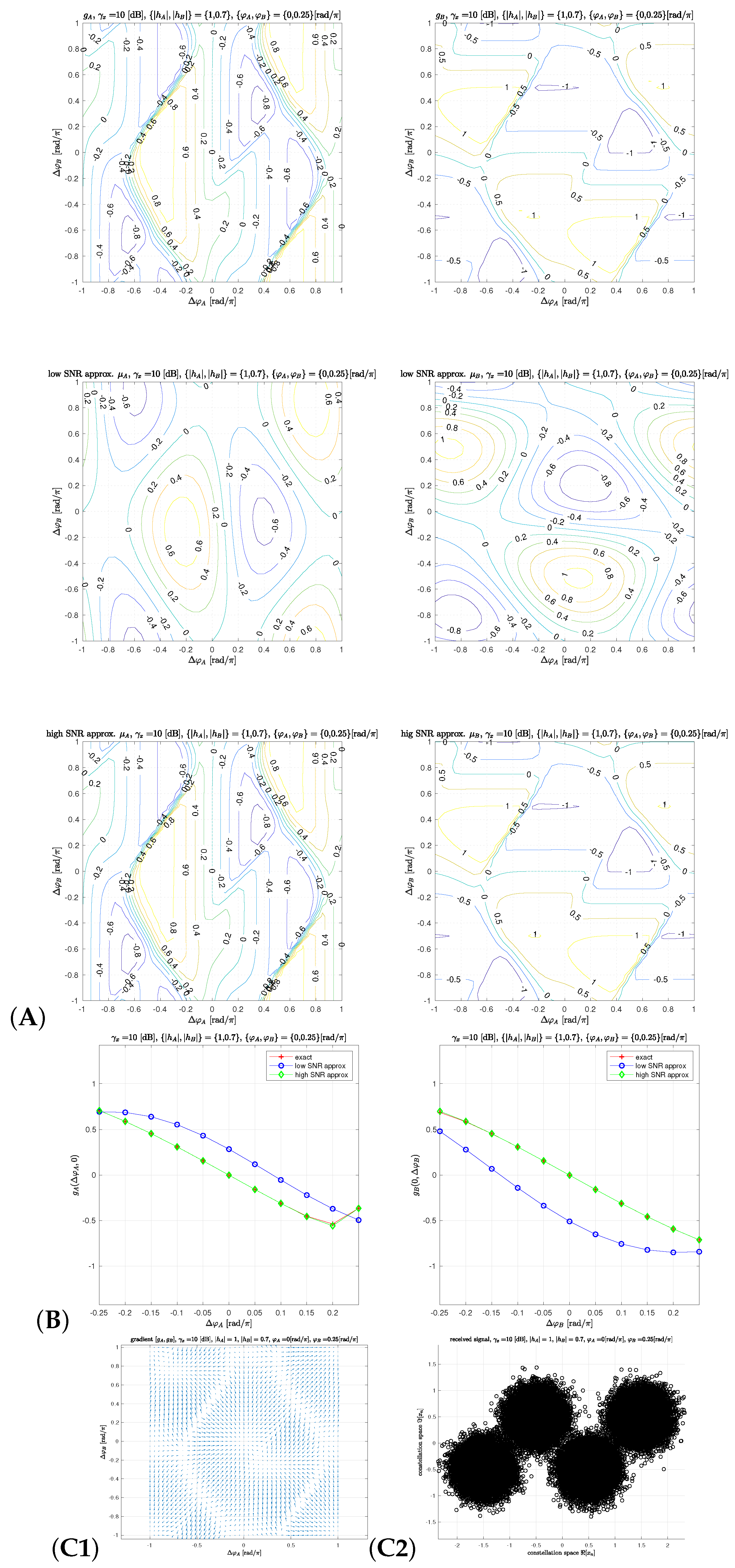
4.1. Equivalent Detector Characteristics

The most important property of the equivalent model, and this is the equivalent characteristic of the gradient indicator function (frequently also simply called equivalent detector characteristics). It is defined as a normalized mean value of the indicator function (gradient) for a fixed local estimate parameter φ ^ and for fixed value of the true channel φ observed in the received signal x ( φ )
K g g ( φ , φ ^ ) = E w , s μ ( φ ^ ) | x = x ( φ ) .
The expectation can be evaluated in a closed-form expression or numerically using Monte Carlo simulation.
The most important properties that we want to investigate are (1) the position of the main stable node, which should ideally give g ( φ , φ ) = 0 for any φ , and (a) the gradient direction g ( φ , φ + Δ φ ) in the plane of all Δ φ , which should ideally direct to the main stable node (the origin) Δ φ = 0 for any φ . Since the feed-back estimators typically have many stable nodes, this requirement is usually relaxed to just a reasonable neighborhood of the main stable node. The resulting ambiguity needs to be resolved by external means (e.g., pilots, or a differential encoding).
The equivalent detector characteristic under various SNRs, selected phase parameter values, and for exact and low/high SNR approximations are shown in Figure 2, Figure 3 and Figure 4. The 3-D contour plots (A) show the overall detector characteristic shape. The 2-D cuts (B) along Δ φ A = 0 or Δ φ B = 0 show the behavior in the vicinity of the main stable node in easier-to-interpret but component-wise perspective. The vector field graphs (C1) show clearly the position of ambiguous stable nodes. We also show an example of received constellation points (C2) for random values of source symbols and AWGN.

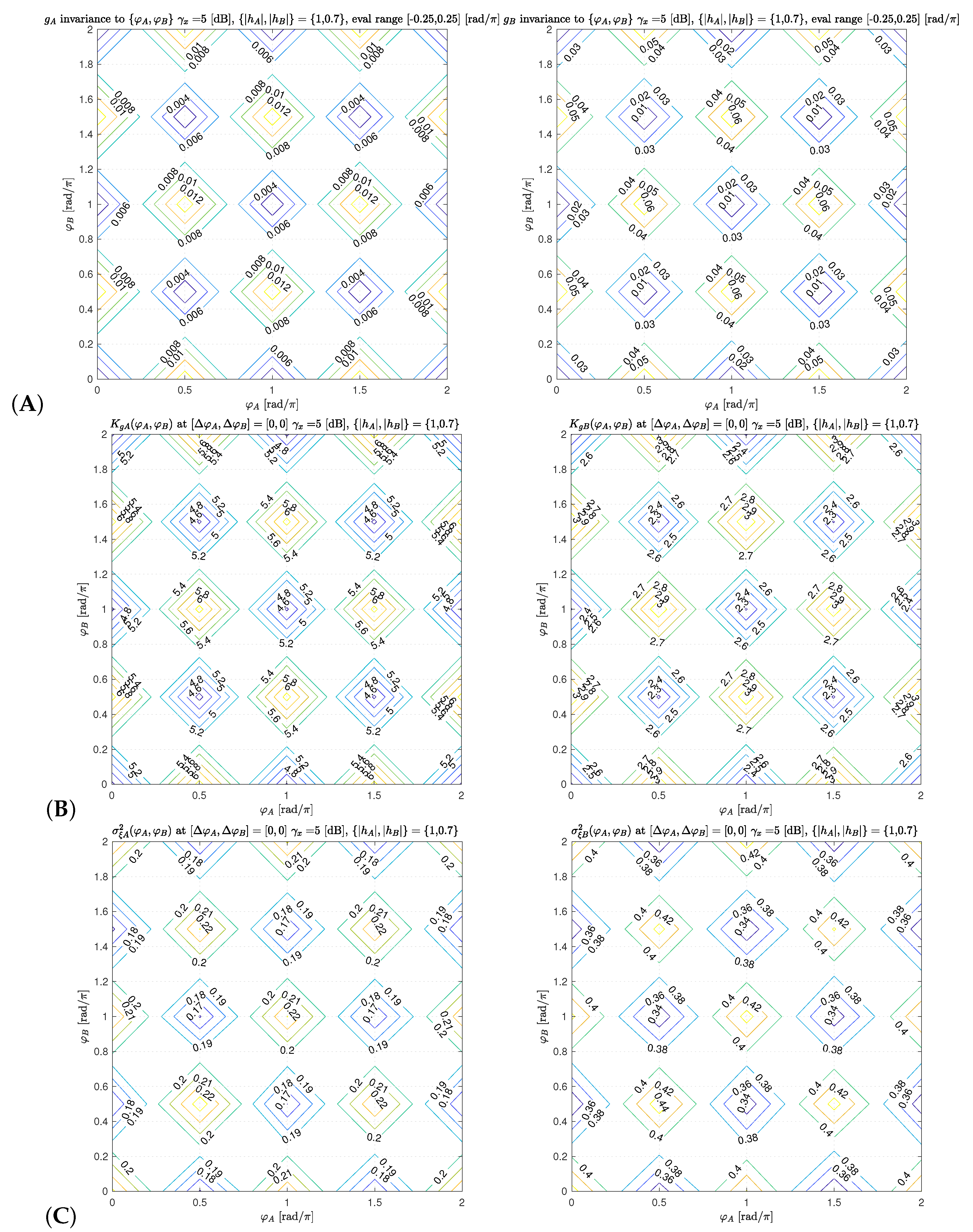
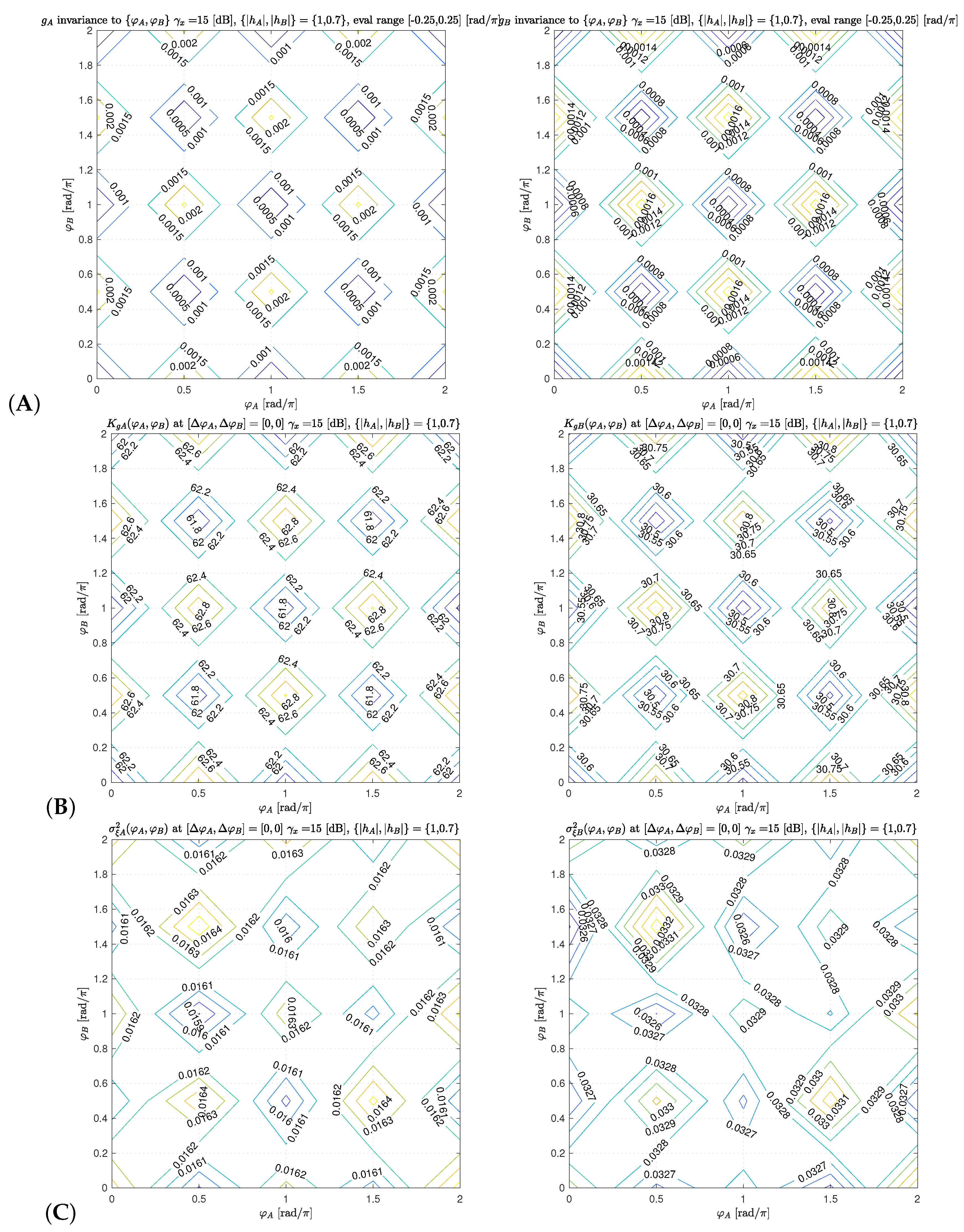
4.2. Invariance to Absolute Channel Component Phases

The invariance of the equivalent model to the absolute channel component phases, i.e., g ( φ , φ + Δ φ ) not being a function of φ , simplifies substantially the dynamic analysis of the feed-back solver [9,10]. Neither exact, nor approximate expressions, for the gradients (see Section 3.2) demonstrate this invariance in an explicit exact manner. A numerical analysis shows that there is a residual dependence, however this is quite negligible mainly in the vicinity of the main stable lock point. We consider this vicinity to be a range of Δ φ A , Δ φ B [ π / 4 , π / 4 ] which is important under normal loop tracking conditions. It is also frequently used in linearized approximations of the loop solution. Very good approximate invariance is shown for all equivalent model characteristics, i.e., the detector characteristics, the detector gain and the equivalent noise variance, in the contour plots Figure 5 and Figure 6. The evaluation of the gain and the variance invariance is simply done by plotting the contours of the variable for all absolute component values φ A , φ B . The evaluation of the detector characteristic invariance is visualized as a contour plot of the mean square difference value over all Δ φ A , Δ φ B [ π / 4 , π / 4 ] where the reference detector shape is the one for φ A = 0 , φ B = 0 .

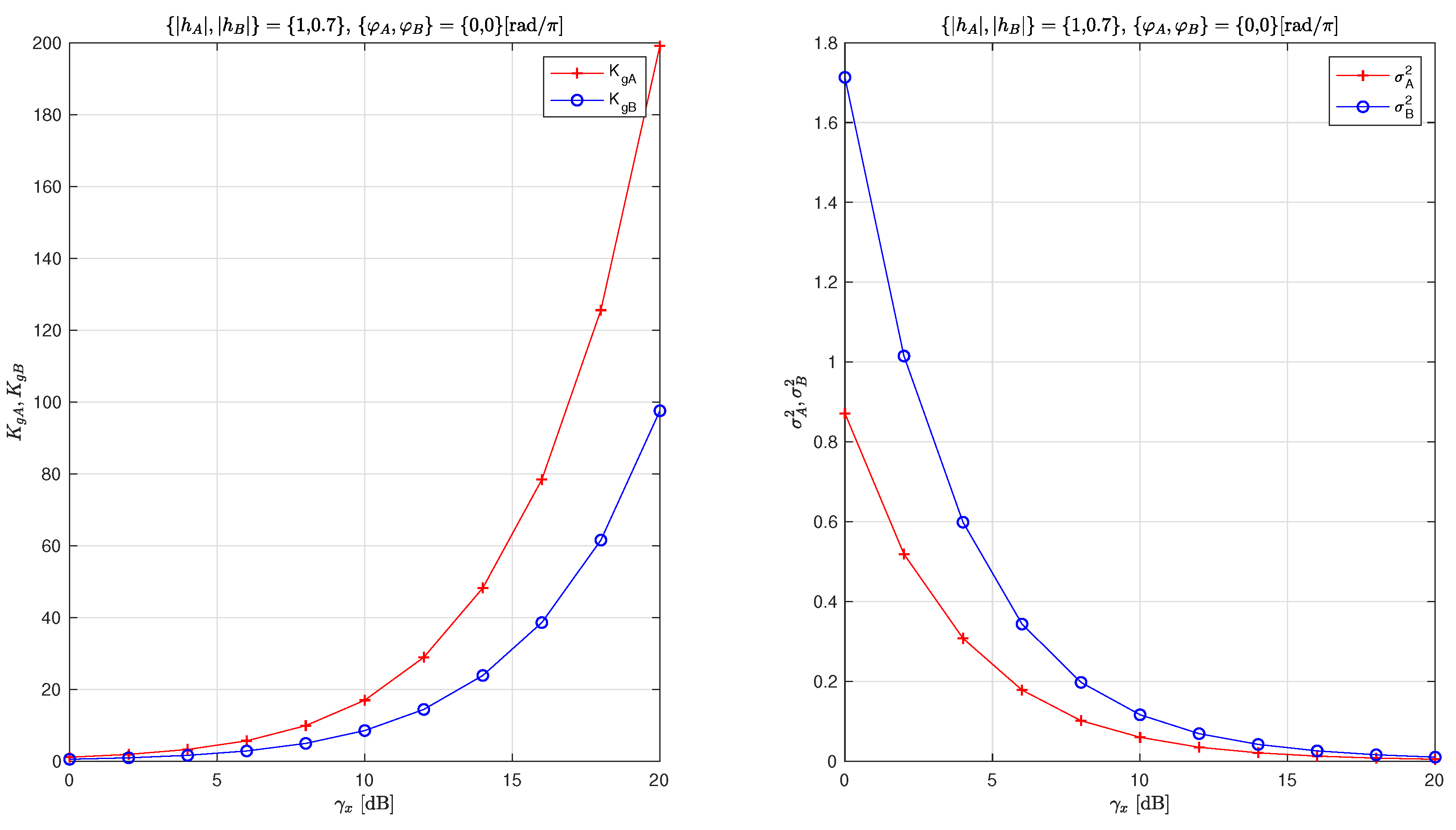
4.3. Detector Gain and Equivalent Noise

The detector gain and the equivalent noise variance are fundamental parameters needed for the analysis of the solver dynamic tracking and convergence properties. Their values are quite numerically invariant to absolute phase values, so their evaluation is done only for φ A = 0 , φ B = 0 . The resulting values over range of SNR are in Figure 7. We can nicely see the component difference caused by unequal values of η A , η B . We also notice a substantial dependence of both values on SNR. This very specific behavior (namely for the gain) needs to be properly respected in the setting of the solver loop overall gain. The loop gain dictates the speed of the convergence and the dynamics response of the loop (the higher gain the faster response). These dynamics properties are thus significantly dependent on the actual SNR.

5. Discussion and Conclusions

5.1. H-Decision Aided H-MAC 2-Source Phase Estimator

We have derived the H-MAC channel phase estimator for 2 BPSK source nodes, which is aided only by the knowledge of H-data decision, i.e., no information on individual source symbols is needed or available at the relay. The estimator is obtained by a marginalization over the hierarchical dispersion. The estimator uses gradient additive update solver and the indicator function (gradient) is derived in exact closed form and in an approximation for low and high SNR.

5.2. Good Tracking Capabilities of Feed-Back Gradient Solver

The (C1) parts of Figure 2, Figure 3 and Figure 4 show the exact solution gradients. We see that the attraction domain of the main stable node (i.e., the region in Δ φ plane, where gradient aims in a correct direction towards the main stable node Δ φ = 0 ) is relatively very wide. As expected there are other stable nodes (not the main one) since the H-constellation and source constellations are rotationally invariant. This is unavoidable in the random data case. It can be resolved only by using rotationally unique pilots or codebook. However, it is instructive to see that the pattern of other stable nodes is (unlike for classical single user PSK case) irregular and depends on true H-MAC channel phases.

5.3. Exact and Low/High SNR Approximation

The exact gradient indicator function solution exhibits desired behavior, mainly the presence of the main stable node at Δ φ = 0 . However, the expression contains complex nonlinear functions which makes its practical implementation difficult. We have investigated low SNR approximation, which contains only quadratic functions of received signal. However, this approximation exhibits a problematic behavior—its main stable node is not located at the origin (see parts (B) and row#2 of parts (C) in Figure 2, Figure 3 and Figure 4). This appears to be caused by an asymmetry in the approximation in two gradient contribution parts that are added together. The first one is left intact but the other one is linearized which clearly makes an imbalance between those two contributions dependent on actual H-MAC phases. On the other hand, the high SNR approximation performs surprisingly well even for moderate-low SNRs. It still contains a nonlinear function, but only easy-to-be-handled sign.

5.4. Invariance to True Absolute Channel Phase

Invariance of the estimator solver to the actual channel phase is a property that greatly simplifies the performance analysis. It means that the equivalent detector characteristic is a function only of the estimation error g ( φ , φ ^ ) = g ( Δ φ ) . Although all forms (exact and approximations) of gradient expression mix components of the received signal (containing both individual true phases) and the individual phase estimate values, the numerical graphical evaluation of the gradient demonstrates only minor differences (see Figure 5 and Figure 6).

Funding

This work was supported by the Ministry of education, youth and sports of the Czech Republic, grant LTC17042.

Conflicts of Interest

The author declares no conflict of interest.

Abbreviations

The following abbreviations are used in this manuscript:
CSEChannel State Estimation
WPNCWireless Physical Layer Network Coding
HDFHierarchical Decode and Forward
SNRSignal to Noise Ratio

References

  1. Sykora, J.; Burr, A. Wireless Physical Layer Network Coding; Cambridge University Press: Cambridge, UK, 2018. [Google Scholar]
  2. Zhang, S.; Liew, S.C.; Lam, P.P. Hot Topic: Physical-Layer Network Coding. In Proceedings of the Twelfth Annual International Conference on Mobile Computing and Networking, Los Angeles, CA, USA, 23–29 September 2006. [Google Scholar]
  3. Koike-Akino, T.; Popovski, P.; Tarokh, V. Optimized Constellations for Two-Way Wireless Relaying with Physical Network Coding. IEEE J. Sel. Areas Commun. 2009, 27, 773–787. [Google Scholar] [CrossRef]
  4. Nazer, B.; Gastpar, M. Compute-and-Forward: Harnessing Interference Through Structured Codes. IEEE Trans. Inf. Theory 2011, 57, 6463–6486. [Google Scholar] [CrossRef] [Green Version]
  5. Sykora, J.; Burr, A. Layered Design of Hierarchical Exclusive Codebook and Its Capacity Regions for HDF Strategy in Parametric Wireless 2-WRC. IEEE Trans. Veh. Technol. 2011, 60, 3241–3252. [Google Scholar] [CrossRef] [Green Version]
  6. Minn, H.; Al-Dhahir, N. Optimal training signals for MIMO OFDM channel estimation. IEEE Trans. Wirel. Commun. 2006, 5, 1158–1168. [Google Scholar] [CrossRef] [Green Version]
  7. Haykin, S. Adaptive Filter Theory, 3rd ed.; Prentice-Hall: Upper Saddle River, NJ, USA, 1996. [Google Scholar]
  8. Spagnolini, U. Statistical Signal Processing in Engineering; John Wiley & Sons: Hoboken, NY, USA, 2017. [Google Scholar]
  9. Meyr, H.; Ascheid, G. Synchronization in Digital Communications; John Wiley & Sons: Hoboken, NY, USA, 1990. [Google Scholar]
  10. Meyr, H.; Moeneclaey, M.; Fechtel, S.A. Digital Communication Receivers, Synchronization Channel Estimation and Signal Processing; John Wiley & Sons: Hoboken, NY, USA, 1998. [Google Scholar]
Figure 1. Two-component H-MAC system.
Information 10 00040 g001
Figure 2. Equivalent detector characteristics for γ x = 5 dB, h A = 1 e j 0 , h B = 0.7 e j 0.25 π . (A) detector components g A ( Δ φ ) , g B ( Δ φ ) (row #1) exact, (row #2) low SNR approximation, (row #3) high SNR approximation; (B) detector components g A ( Δ φ A , 0 ) , g B ( 0 , Δ φ B ) ; (C1) gradient directions (exact); (C2) random received constellation points.
Information 10 00040 g002
Figure 3. Equivalent detector characteristics for γ x = 10 dB, h A = 1 e j 0 , h B = 0.7 e j 0.25 π . (A) detector components g A ( Δ φ ) , g B ( Δ φ ) (row #1) exact, (row #2) low SNR approximation, (row #3) high SNR approximation; (B) detector components g A ( Δ φ A , 0 ) , g B ( 0 , Δ φ B ) ; (C1) gradient directions (exact); (C2) random received constellation points.
Information 10 00040 g003
Figure 4. Equivalent detector characteristics for γ x = 15 dB, h A = 1 e j 0 , h B = 0.7 e j 0.25 π . (A) detector components g A ( Δ φ ) , g B ( Δ φ ) (row #1) exact, (row #2) low SNR approximation, (row #3) high SNR approximation; (B) detector components g A ( Δ φ A , 0 ) , g B ( 0 , Δ φ B ) ; (C1) gradient directions (exact); (C2) random received constellation points.
Information 10 00040 g004
Figure 5. Absolute component phase invariance of (A) detector characteristics, (B) detector gain and (C) equivalent noise variance, γ x = 5 dB.
Information 10 00040 g005
Figure 6. Absolute component phase invariance of (A) detector characteristics, (B) detector gain and (C) equivalent noise variance, γ x = 15 dB.
Information 10 00040 g006
Figure 7. Equivalent detector gain and equivalent noise variance as a function of SNR.
Information 10 00040 g007

