Article

Automatic Wireless Signal Classification: A Neural-Induced Support Vector Machine-Based Approach

1
Institute of Microelectronics Chinese Academy of Sciences, Beijing 10029, China
2
School of Electronic, Electrical and Communication Engineering, University of Chinese Academy of Sciences, Beijing 100049, China
*
Author to whom correspondence should be addressed.
Information 2019, 10(11), 338; https://doi.org/10.3390/info10110338
Submission received: 10 October 2019 / Revised: 25 October 2019 / Accepted: 28 October 2019 / Published: 30 October 2019

Abstract

:
Automatic Classification of Wireless Signals (ACWS), which is an intermediate step between signal detection and demodulation, is investigated in this paper. ACWS plays a crucial role in several military and non-military applications, by identifying interference sources and adversary attacks, to achieve efficient radio spectrum management. The performance of traditional feature-based (FB) classification approaches is limited due to their specific input feature set, which in turn results in poor generalization under unknown conditions. Therefore, in this paper, a novel feature-based classifier Neural-Induced Support Vector Machine (NSVM) is proposed, in which the features are learned automatically from raw input signals using Convolutional Neural Networks (CNN). The output of NSVM is given by a Gaussian Support Vector Machine (SVM), which takes the features learned by CNN as its input. The proposed scheme NSVM is trained as a single architecture, and in this way, it learns to minimize a margin-based loss instead of cross-entropy loss. The proposed scheme NSVM outperforms the traditional softmax-based CNN modulation classifier by managing faster convergence of accuracy and loss curves during training. Furthermore, the robustness of the NSVM classifier is verified by extensive simulation experiments under the presence of several non-ideal real-world channel impairments over a range of signal-to-noise ratio (SNR) values. The performance of NSVM is remarkable in classifying wireless signals, such as at low signal-to-noise ratio (SNR), the overall averaged classification accuracy is > 97% at SNR = −2 dB and at higher SNR it achieves overall classification accuracy at > 99%, when SNR = 10 dB. In addition to that, the analytical comparison with other studies shows the performance of NSVM is superior over a range of settings.

1. Introduction

With the development of new technologies, such as extreme mobile broadband (eMBB), multimedia terminals in cellular networks has triggered the need of providing higher bandwidth and reliable links in wireless environments. However, the available radio spectrum is limited and the current technologies have been shown to have low spectrum efficiency. Therefore, there is a need to design self-organizing, adaptive, and non-cooperative wireless technologies to enable efficient radio resource utilization.
Automatic Classification of Wireless Signals (ACWS), which is an intermediate step in signal detection and demodulation, is used for identifying interference sources and efficient radio spectrum management in several military and non-military applications. ACWS is an essential process in achieving higher data rates by enabling adaptive transmission settings across varying channel conditions without any prior knowledge of the received signal [1]. In several military applications, it is used for surveillance of adversary attacks and electronic warfare purposes. Automatic Classification of Wireless Signals generally involves two steps: pre-processing of received signals and classification algorithm design. In the literature, ACWS techniques are broadly categorized into two main approaches: likelihood-based (LB) and feature-based (FB). Likelihood-based approaches are based on hypothesis testing, comparing the likelihood functions of received signals to classify different modulations by employing an average likelihood ratio test ALRT [2,3,4,5], a generalized likelihood ratio test (GLRT) [2,3,4] and a hybrid likelihood ratio test (HLRT) [2,3,4]. These decision theoretic approaches achieve optimal performance, but at the cost of high computational complexity. Therefore, feature-based approaches are preferred in practice as suboptimal classifiers. In FB approaches, feature extraction is performed at a pre-processing unit followed-by a classification algorithm that classifies the received signal based on the features extracted at the pre-processing step. A general block-wise architecture of the feature-based classifier is given in Figure 1. In Reference [6], Azzoz and Nandi proposed a decision tree-based classifier for automatic classification of digital and analogue modulation signals with spectral features, such as instantaneous amplitude, phase and frequency as its input feature vectors. Swami and Sandler [7] proposed a hierarchal decision tree-based classifier with fourth order cumulants as their input features. In Reference [8], Wang combines the instantaneous spectral features and fourth order cumulants of received signals as input features for a PSO-based support vector machine. The use of cyclostationay features for signal classification has been reported by Reference [9] in detail. Machine Learning classifiers such as decision tree (DT) [10], Support Vector Machine (SVM) [11], and k-nearest neighbor (KNN) [12] have been used widely as shallow classifiers to classify wireless signals based-on the aforementioned feature set. However, these conventional FB approaches mainly rely on expert knowledge which may perform well on the proposed solution but suffers from a lack of generality and time-consumption with high computational complexity. This is due to their primary dependence on handcrafted specific features, which may not be suitable for different modulation sets and various adaptive channel conditions.
To obviate manual feature engineering, deep learning (DL) [13], which is a sub-field of machine learning, has been used in several studies. A DL model has the ability to learn the features automatically without relying on any mathematical model or expert knowledge. A fully connected neural network and the hyperparameters can be tuned by conducting engineering experiments over the underlying task. Deep learning [14] has shown remarkable performance in several fields (not limited to), such as image classification [15,16,17], natural language processing (NLP) [18] and drug discovery [19,20]. Recently, these deep learning-based approaches such as Convolutional Neural Networks (CNNs) [21,22], stack autoencoders [23] and deep belief networks [24] have been applied for modulation classification as well as performing physical layer low-level tasks in wireless communication. Since these deep learning-based methods enable the receiver to learn different features automatically from the input received signal latent space, in several studies, neural networks have been employed as decision classifiers for a pre-processed received signal. For example, Wong and Nandi, in Reference [6], used an artificial neural network (ANN) with a genetic algorithm (GA) for automatic modulation classification. In their study, the GA was used to select the best features from a statistical and spectral feature set. In Reference [25], cumulants are used for classification features with Convolutional Neural Networks (CNN). Oshea [21] used CNN directly for modulation classification and achieved a promising performance compared to previous feature-based neural network approaches. In Reference [26], CNN was used to learn features separately, which are then used as input for a Support Vector Machine classifier. However, all of the aforementioned methods based on Convolutional Neural Networks (CNN) used the softmax activation function (multinomial logistic regression) for the classification decision. An alternative to softmax is the Support Vector Machine (SVM), which has been applied to several classification tasks [27]. The use of SVMs in combination with Convolutional Neural Networks (CNN) have been proposed in the past as part of a multistage process, mainly for image classification [28]. In which, a deep Convolutional Neural Network was first trained using supervised objectives to learn good invariant hidden latent representations. Then, these corresponding hidden features of data samples are treated as input to SVMs [29]. This technique usually improves the performance slightly, but in such settings, the low-level features have not been fine-tuned with respect to the Support Vector Machine’s objective. Therefore, in this paper, a novel feature-based algorithm Neural-Induced Support Vector Machine (NSVM) is proposed, in which we replace the softmax layer of the CNN model with a SVM. The objective function of the Support Vector Machine (SVM) is rewritten to train CNN and SVM as a combined architecture. In this way, the proposed scheme learns to minimize margin loss rather than cross-entropy loss. The proposed schemes show remarkable improvement in the performance, as compared to the traditional CNN-based model for classification of wireless signals.
The remainder of the paper is organized as follows: Section 2 introduces the system model. A detailed explanation of Convolutional Neural Networks, the Support Vector Machine and the proposed scheme NSVM for Automatic Classification of Wireless Signals is presented in Section 3. Section 4 outlines the simulation experiment results and discussion. Finally, the overall study is concluded in Section 5.

2. Signal Model and Problem Statement

The classification of wireless signals can be generally formulated as an n-class classification problem, where n is the number of different modulation schemes. In this study, only digital modulation schemes are considered, these are BPSK, 4ASk, QPSK, 8PSK, QAM16, QAM64.
A general description of a wireless communication system is given as a system that transmits information from one point to another point via a wireless medium. The received baseband signal at the output of the matched filter can be expressed as:
r = k s m ( k ) · h ( t k T ) ,       m = 1 , , M ,       1 t T
where, s m is the i . i . d symbol stream carried by constellation m M , and T is the period of the received signal r . The physical link between each transmitter and receiver is classically modeled as a delayed tapped channel model, expressed as:
h ( t ) = A ( t ) · e i ( 2 π f c + φ ) · δ ( t τ )
where, v ( t ) stands for additive white Gaussian noise (AWGN) with unknown variance σ v 2 . The received signal whose modulation type and symbol energy are unknown is pre-processed blindly by assuming to be drawn from a minimum-energy constellation, which is true in the case of almost all the modulation types. The discrete-time samples r ( n ) , at the output of the pre-processing unit are given as:
r ( n ) = u = 1 U y u ( n ) + v ( n )
where, A ( t ) is the amplitude, f c represents the carrier frequency, φ is the phase and τ is the delay. We can rewrite the received multipath signal at the receiver as follows:
r ( t ) = k = 0 L 1 r ( t k ) · h ( k ) + v ( t )
where, r u ( n ) is the u t h component of the signal.
r u ( n ) = A ( t ) · e i ( 2 π f r c n + φ ) k s u ( k ) · h ( n T s k T τ )
T s denotes the sampling period and f r c is the residual carrier frequency offset (CFO) for the received signal u.

3. Convolutional Neural Networks (CNN), Support Vector Machine (SVM) and Neural-Induced Support Vector Machine (NSVM)

In this section, the Convolutional Neural Networks are briefly described first, followed by the Support Vector Machine details. The focus is to inspect their internal structures to provide insights into their respective strengths and weaknesses on the present modulation classification task. This analysis will lead to proposing NSVM, which combines the strengths of the two methods. For example, SVMs can produce good decision surfaces if the input representation is reasonably well-behaved, but, with their fixed architecture, they cannot learn to extract relevant features so as to handle complicated invariances in the input. Conversely, Convolutional Neural Networks can learn invariant local features that are appropriate for wireless signal classification, but the top layers seem to produce suboptimal classification surfaces.

3.1. Convolutional Neural Networks

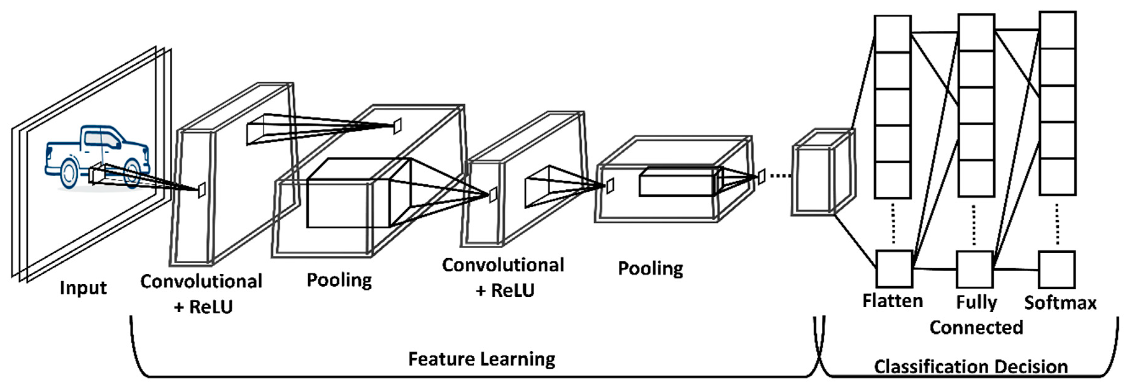
In 1988, LeCun and Bottou proposed LeNet 5 [30] for recognizing handwritten digits which lay out the foundations for modern Convolutional Neural Networks. The study carried out by Hubel and Wiesel in Reference [19] explains how mammals visually perceive by using the layer architecture of neurons in the brain. Similar to that, a typical CNN is also composed of layered architecture, which is why CNN are called biological-inspired networks. A basic architecture of a Convolutional Neural Network is shown in Figure 2.
The layered CNN architecture consists of several layers in which each layer transforms the input into a meaningful representation. The detailed description of Input layer, Convolutional Layer, pooling layer, fully connected layer and SoftMax are discussed below.

3.1.1. Input Layer

The raw images can be directly fed to the network via the Input layer. The images are represented by its pixel values at the input layer.

3.1.2. Convolutional Layer

The convolutional layer is also called the up-sampling layer as it extracts features from the input data. The features extraction is performed by several convolutional filters, as different kernels represent different features of the input data. The number of extracted features is directly related to the number of convolutional kernels in the up-sampling layer. One can always learn better hidden representation of input data by increasing the depth of the convolutional layer. A convolutional operation can be expressed as:
h k m = f ( x m w k m + b k m )
x m w k m ( i ) = l = + x ( l ) w k m ( i l )
where, x is the set of inputs and w represents the kernel. To achieve the nonlinear mapping of the kernel outputs, an activation function f ( . ) is employed in Equation 6. There are many activation functions such as Sigmoid, tanh and Rectified Linear Unit (ReLU). In this study, ReLU is used as the activation function with the convolutional Layer.
f ( x ) = { x                             i f   x > 0 0                               i f   x 0

3.1.3. Pooling Layer

The pooling layer is also called the down-sampling layer as it sums up information and maps the dominant response within the specific local region of the respective field. Max pooling is used in this study, which can be represented as:
h k m + 1 ( i ) = max ( h m k ( n m + 1 ( i 1 ) + 1 ) , h m k ( n m + 1 ( i 1 ) + 2 ) h m k ( n m + 1 ( i 1 ) + N ) )
where, N is the length of pooling windows and n m + 1 is called stride and represents the margin between two pooling windows.

3.1.4. Fully Connected Layer

The feature maps learned by the convolutional or pooling layer is flattened to a one-dimensional array of values. It is also called the dense layer, in which each neuron is connected to the output layer by a learnable parameter.

3.1.5. SoftMax Layer

The final output layer has a number of neurons and an equal number of classes in a classification task. It specifies the probability distribution of each class. The Input to the SoftMax layer can be written as:
a n = m h m w m n
The probability of each class is specified as:
P i = exp ( a n ) i k exp ( a i )
The input sample is predicted by taking the maximum overall probabilities.
i = arg max P i

3.1.6. Loss Function

The loss function or objective function of CNN is defined as J ( . ) . In supervised learning we are to optimize this loss function by minimizing the difference between the output prediction and the true labels. This can be written as:
arg min W , b   J ( W , b )
This is done by a gradient descent algorithm, with the following updates moving backwards in the network during training.
W : = W α d J ( W , b ) d W
b : = b α d J ( W , b ) d b
where, α is the learning rate.

3.2. Support Vector Machine

The basic idea of the SVM classifier is to transform the input space into a higher dimensional space by non-linear transformation, then use the risk minimization criteria to construct an optimal separating hyperplane in the new space. SVM optimizes the following optimization problem:
P 1 :                     min w ,   b ,   ξ 1 2 w 2 + C i = 1 n ξ i s . t .                 y i ( w T · Φ ( x i ) + b )   1   ξ i ξ i 0 ,   i = 1 ,   ,   n
where, ( ( x 1 ,     y 1 ) ,   ,   ( x M ,     y M ) ( x 1 ,     y 1 ) ,   ,   ( x M ,     y M ) ) are M samples for x i , in which the class labels y ( + 1 , 1 ) l are either positive or negative, which can be separated by the hyper-plane ( w T · Φ ( x i ) + b ) , Φ   :   N     F is the mapping function of the input data into some higher dimensional Hilbert space , where W   is orthogonal to the separating hyper-plane in that space, C is a positive number and ξ i is the error in the soft margin. ξ i   0 are the non-zero slack variables introduced to enable the learning algorithm to deal with data that could not be precisely separated, such as data with noise. b     is the bias and C     is a penalty factor used to establish a trade-off between maximizing the margin and minimizing the classification error. By taking the Lagrangian of P 1 , we have:
( w , b , α , ξ ) = 1 2 w 2 +   C i = 1 n ξ i   i = 1 l α i [ y i ( w T · Φ ( x i ) + b ) 1 + ξ i ]
Minimizing ( w , b , α , ξ ) w.r.t to w , b , α , ξ respectively, we get the dual form of P 1 given as:
D 1 :   a r g   max α i   0 i = 1   M α i   1 2 i = 1 M j = 1 M α i α j y i y j Φ T ( x i ) ,   Φ ( x j ) = a r g   max α i   0 i = 1   M α i   1 2 i = 1 M j = 1 M α i α j y i y j κ ( x i ,   x j )     s . t   0 α i C   i ,   i = 1 M α i y i = 0
where, κ ( . ) is a positive defined kernel, representing the dot product κ ( x i ,   x j ) =   Φ ( x i ) ,   Φ ( x j ) of the data point in . The strategy of a kernel is to map the training data into the feature space x i Φ (   x i ) to separate them from the origin with maximum margin, which map the features to higher space, a Gaussian kernel is being employed in this paper. The Gram matrix of the Gaussian kernel is given as:
G = ( y i y j κ ( x i , x j ) ) i ,   y = 1 l
Which is a positive semi-definite that ensures that the maximal margin optimization has a unique solution that could be found efficiently. This effectively rules out the problem of being stuck in local minima that has been mostly encountered while training neural networks. Because of the optimality relations between the primal and dual problem, the hyperplane that separates the data in the high dimensional space, determined by the normal w * and the intersection with the axis, b * , satisfies the following:
w * =   i = 1 M α * i y i Φ ( x i ) b * = 1 max { y j = 1 } ( w * ) t Φ ( x i )
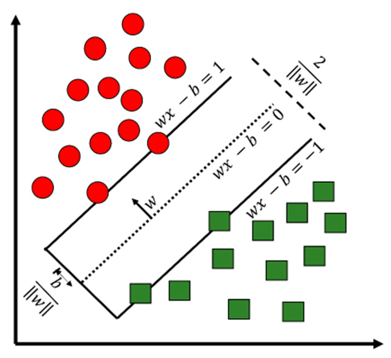
A SVM separating the hyperplane for binary classification is shown in Figure 3. The function used to classify a new point X can be written as:
f ( X ) = sign ( i = 1 M α i * y i k ( x i ) + b * )

3.3. Neural-Induced Support Vector Machine (NSVM)

In this paper, the NSVM is introduced for the automatic classification of wireless signals based on their modulation formats by combining Convolutional Neural Networks and the Support Vector Machine. The architecture of NSVM is shown in Figure 4. As it can be seen from Figure 4, the softmax layer of the Convolutional Neural Networks is replaced by the Support Vector Machine. The Support Vector Machine takes the entire feature layer as input and outputs the label of the input sample. The output expression can be written as:
f ( x ) = i = 1 l ( α i * α ) K ( φ ( x i | θ ) , φ ( x | θ ) ) + b
where K ( . , . ) is the kernel function of the Support Vector Machine.
To find a suitable f , the system must find a representation of the input data in z that codes the feature most relevant for estimating the desired output. The training samples x i is replaced by the feature vector φ ( x i | θ ) . The primal problem of SVM can be written as:
P 1 :                     min w ,   b ,     ξ   1 2 w 2 + C i = 1 n ξ i s . t .                 y i ( w T . φ ( x i | θ ) + b )   1   ξ i ξ i 0 ,   i = 1 ,   ,   n
Corresponding to the dual problem formulates as:
D 1 :   min θ   a r g   max α i   0 i = 1   M α i   1 2 i = 1 M j = 1 M α i α j y i y j φ T ( x i | θ ) ,   φ ( x j | θ ) = min θ   a r g   max α i   0 i = 1   M α i   1 2 i = 1 M j = 1 M α i α j y i y j K ( x i | θ ,   x j | θ )     s . t   0 α i C   i ,   i = 1 M α i y i = 0
The two goals of training are to find α * that maximizes the above problem and also the weights θ of the neural network which minimizes Equation (24). This hybrid model is trained as single architecture rather than training them separately and then combining them offline for classification.

4. Simulation Results and Discussion

In this section, the performance of the proposed scheme is investigated against several non-ideal channel conditions such as frequency offset, phase offset, timing offset, varying symbol number as well as different Doppler shifts. An analytical comparison is also provided with previously proposed different learning-based modulation classifiers.

4.1. Dataset

In this paper, the following M = ( B P K S , 4 A S K , Q P S K , 16 Q A M , 64 Q A M ) modulation schemes were considered. The transmitted bit-stream was generated randomly to ensure each has equal probability. The received signal was pre-processed at the receiver end to obtain a complex based-band signal. The In-Phase-Quadrature (I-Q) samples of the received signal were sampled simultaneously to a frame of length N. They are combined later in a 2 X N matrix and input to CNN for feature extraction. In this study, the value of N is 2048 but some experiments are performed with N = 1024, 512. This is done by varying the number of symbols in the frame. A segment has the same results as that of a full observation. In this way, the proposed classifier would be independent of N. The range of AWGN noise with signal-to-noise ratio (SNR) = −8 dB to +8 dB in the dataset. For each modulation scheme and SNR values, 10,000 realizations of the received signal are generated according to the model described in Section 2. The rest of the parameters are summarized in Table 1 in detail.

4.2. Training and Validation Performance

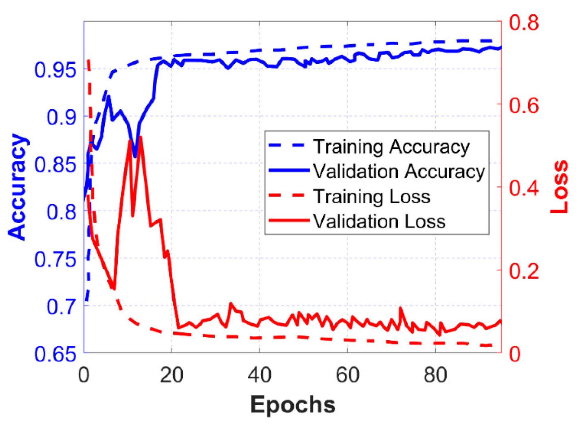
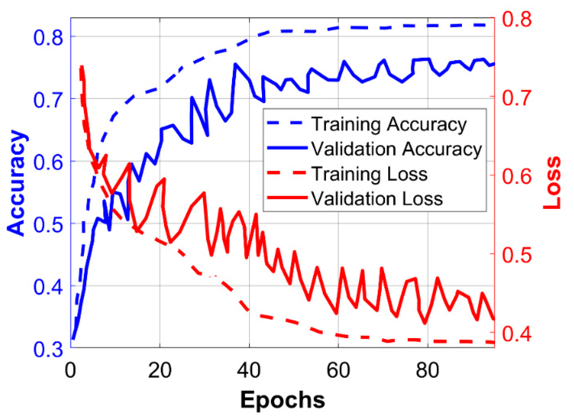
In the following experiment, the proposed classifier NSVM, which is a hybrid combination of CNN and SVM is trained and validated by using offline deployment. In order to analyze the performance, the accuracy and loss curves of training and cross-validation are plotted in Figure 5. Similar experiments are performed with a traditional CNN model with the softmax classifier in its last layer, and the results are plotted in Figure 6. The CNN settings used here are the same in both cases, as shown in Figure 4, expect one is trained with Gaussian SVM and the other one is trained with softmax as the decision classifier. The performance of NSVM is better than the traditional CNN model as the accuracy and loss converges to their minima and maxima quickly. Along with that, these results show that it smoothens as training progresses, which shows the effectiveness of the proposed scheme. This also reduces the cost of training for the proposed model. However, in the case of CNN with softmax, the classifier performance is hardly stable and satisfactory, as can be seen in Figure 6.

4.3. Basic Classification Performance

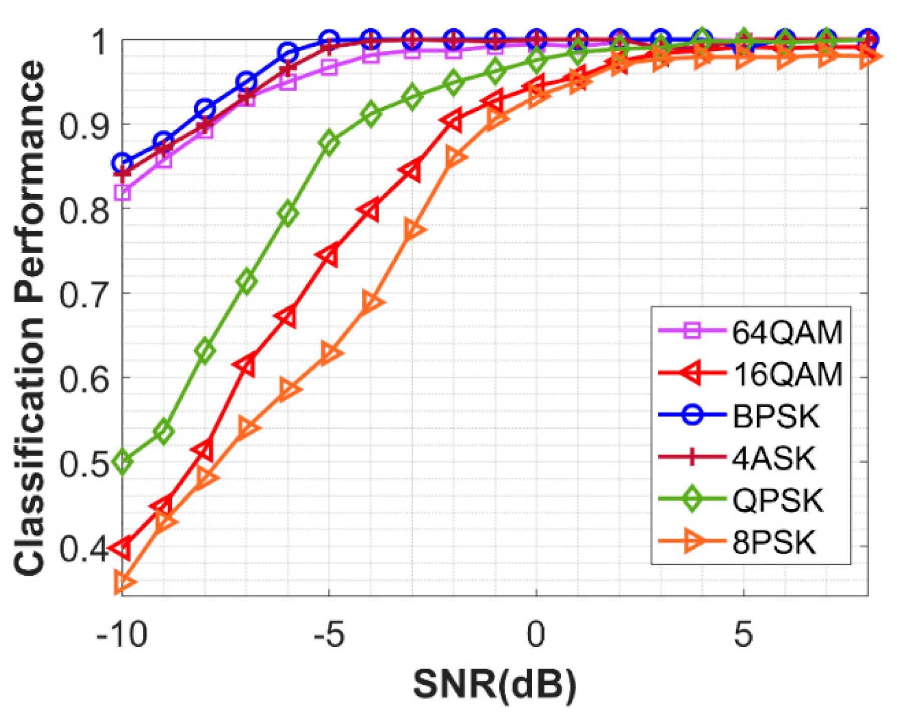
The performance of NSVM under ideal channel conditions for individual modulation schemes are shown by Figure 6. The confusion matrix at SNR = −4 dB and SNR = 0 dB is given by Table 2. One-dimensional modulation schemes 4ASK and BPSK are easily recognizable even at low SNR. However, the performance NSVM for higher dimensional modulation types in the dataset requires a high signal-to-noise ratio (SNR) to achieve satisfactory performance. The performance of QAM 16, QPSK and 8-PSK is lower than QAM64 in the low SNR region. Similar results were reported in Reference [6], in which QAM64 achieves better performance than QAM16 with different learning-based modulation classifier methods based on machine learning techniques. This is due to the fact that the distinctive features learned by CNN hidden layers are increased in the case of high modulation, such as QAM64. The performance of QPSK and 8PSK degrades with a decrease in the SNR of received signals. However, at SNR > 3 dB, the algorithm manages to achieve classification accuracy of <98%. In this experiment, the performance of NSVM in classifying individual modulation schemes has been analyzed. The receiver is assumed to have the information of all the parametric information about the signal (e.g., if there is any phase offset, symbol timing offset, frequency offset, etc.), except the modulation format needs to be inferred. In our experiments, by default, the value of N is 2048, in case a change will be mentioned. The result of classifying six different modulation schemes is given Figure 7. The modulation schemes 4Ask and BPSK can be easily classified by our model in the dataset. However, the distinctive features learned by CNN are increased in the case of QAM 64. Therefore, it achieved performance much better than QPSK, 8PSK, and QAM 16. The performance of QAM 16 is misclassified at low SNR due to its similar constellation map with QAM64. However, similar behavior has been seen in QPSK, as they required higher SNR to be classified correctly. Therefore, in this section, confusion matrices at SNR = −4 dB and SNR = 0 dB are given in Table 2 and Table 3, respectively. As it is clear from the tables, more misclassification occurs in higher order modulation due to low SNR. In the low SNR regime, QPSK is often misclassified as the 8PSK, this can be explained by the assumption in which QPSK is taken as subset 8PSK. In order to improve the performance of the proposed scheme, more MPSK/M-ary QAM modulation schemes can be considered, which will enable the CNN model to gather more information about the same constellation but different symbol order sequences. The following experiment was conducted with a fixed number of symbols in the frame. In the next section, the different symbol length effect is discussed.

4.4. Performance of NSVM with Different N

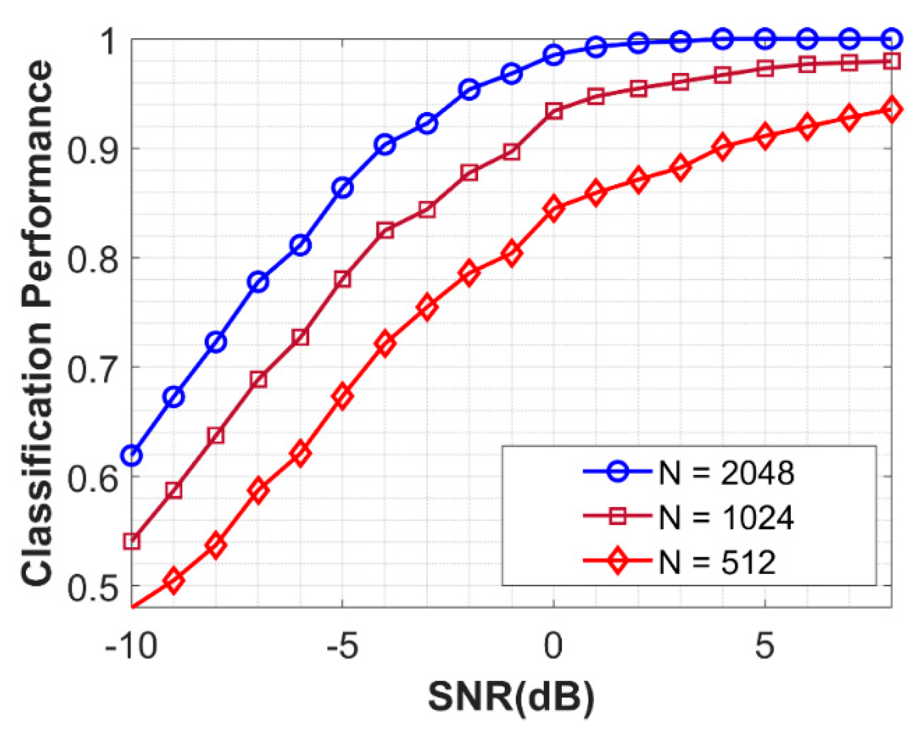
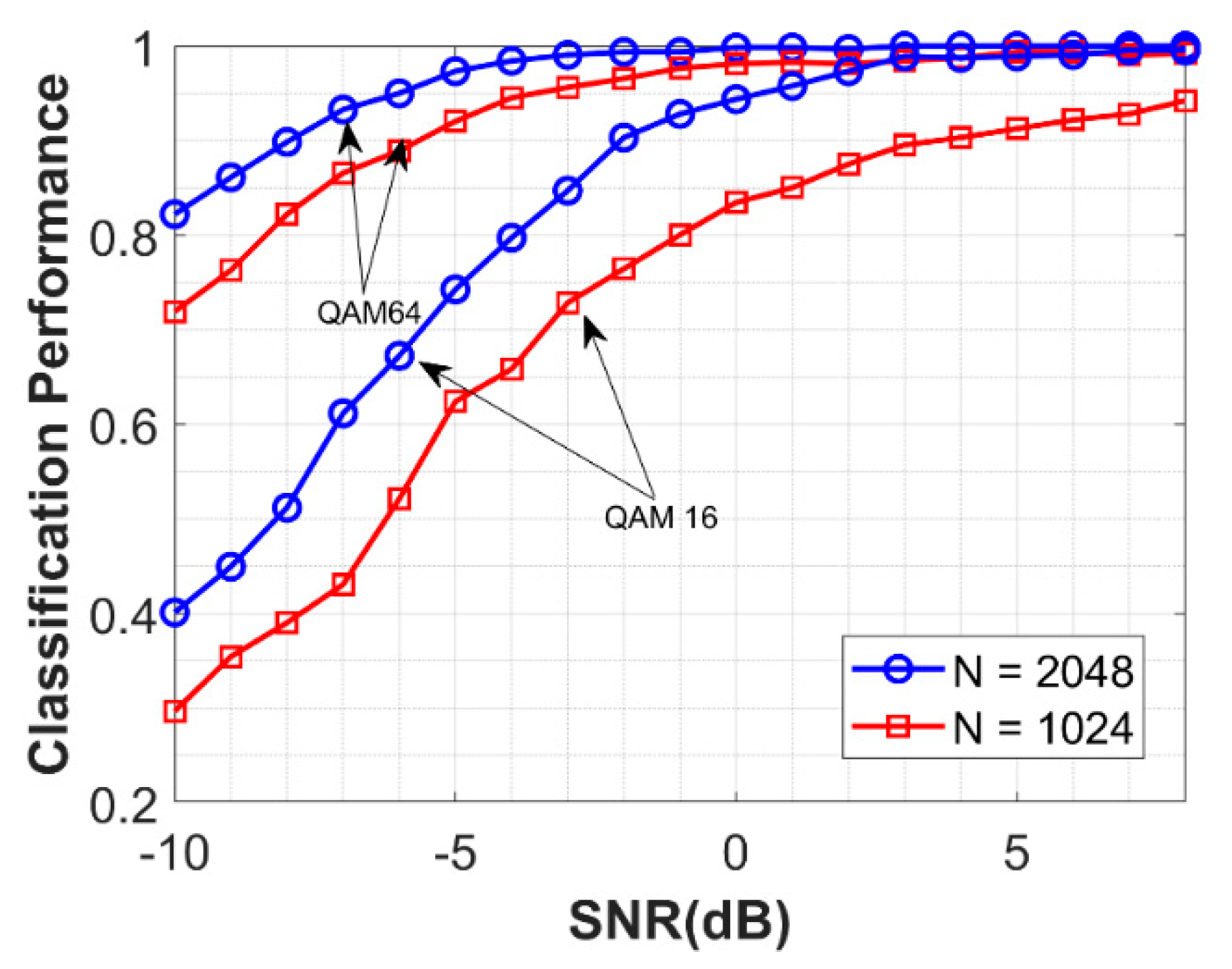
The performance of the proposed schemes with different numbers of symbols is analyzed in this section. The overall averaged accuracy with symbol Number N = 2048, 1024 and 512 is plotted in Figure 8. The performance achieved reasonable degradation in classification accuracy as the number of space decreased. Another observation made here is to relate the performance of the proposed algorithm NSVM with higher order modulation. It can be seen from Figure 9 that the performance of the proposed QAM16 and QAM64 is compared with different symbol numbers. The proposed scheme performed better for higher order modulation due to more information being extracted from the constellation map by CNN, as well as a greater number of symbols.

4.5. Performance of NSVM with Different Channel Impairments

Signal classifiers don’t have any prior knowledge of when and where a transmission will occur. Hence, a wide signal is pre-processed to a based-band type, which is then considered for classification. There might be many channel variations still there due to the estimation error at the pre-processing. Therefore, to analyze the robustness of NSVM, the experiments are carried out on the test data with four different channel impairments, e.g., Carrier Frequency Offset, Timing Offset, Phase Offset and Velocity. The test set for each of these parts is generated separately, which consists of 2000 test realizations for each channel variation at each SNR value being generated for this section.
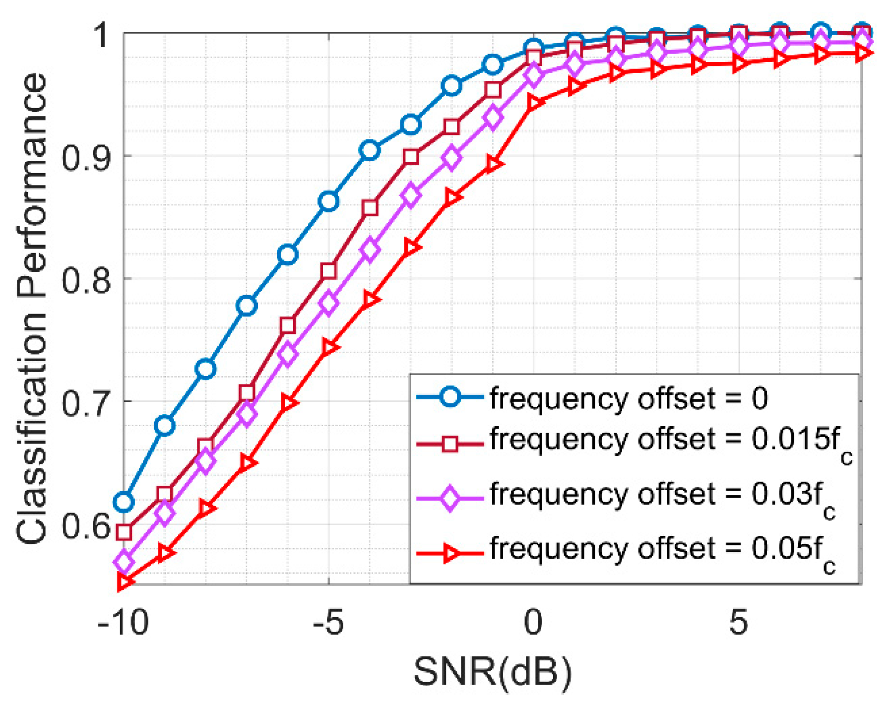
Effect of Carrier Frequency Offset: The performance of NSVM due to different carrier frequency offset is shown in Figure 10. It can be observed that with the increase in carrier frequency, the performance of the proposed classifier degrades significantly. However, the performance is worse at a low SNR. This is due to the fact that the model is not using that data with offset. However, the performance of the proposed scheme at higher SNR manages to achieve reasonable performance. This is due to the fact that the higher order modulations are insensitive to offset in the carrier. To compensate the performance at a lower order, the proposed model can be retrained on the data, having random frequency offsets.
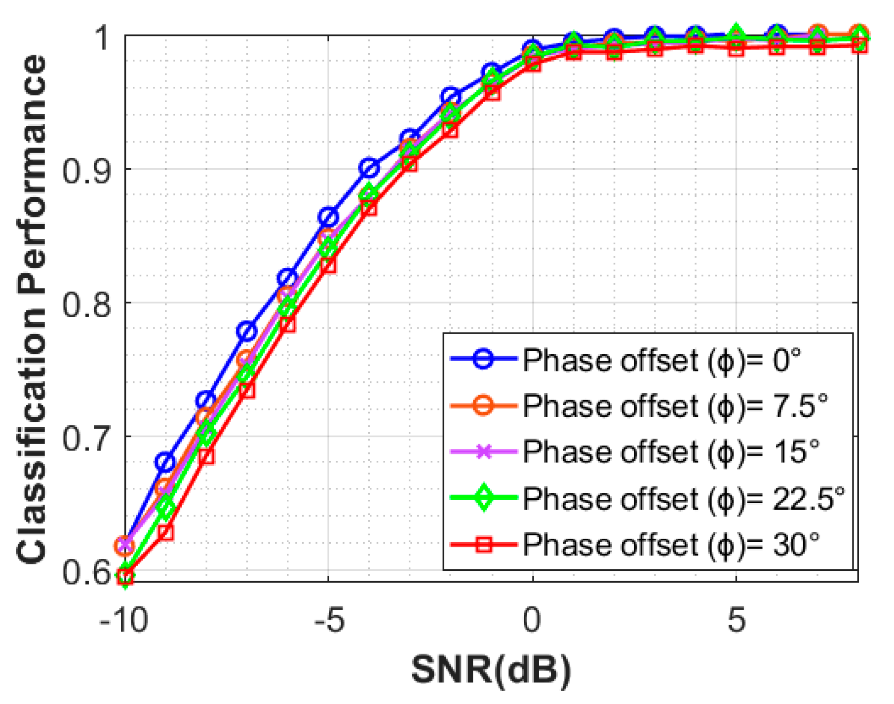
Effect of Phase Offset: In this section, the effect of phase offset observed is investigated. Since the prior knowledge of the phase offset is symmetric; therefore, the influence of positive and negative deviations is the same. The performance of NSVM is observed for the test with the following Δ P = ( 0 , 7 5 , 15 , 22 5 , 30 ) phase offsets in the received signal. The performance of NSVM with Δ P is given by Figure 11. The algorithm generalizes better despite different phase offsets, as the performance remains the same; however, there are slight changes in the performance at low SNR values.
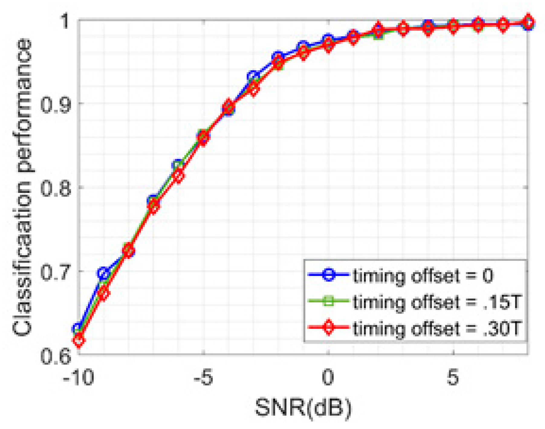
Effect of Timing Offset: Next, the performance of timing offset in the received symbol is discussed in Figure 12. Since, the proposed architecture considers 256 input symbols in a frame as an input, therefore, this effect can easily be compensated. However, this may not compensate for the bit-error rate due to the loss of information despite the correct signal classification.
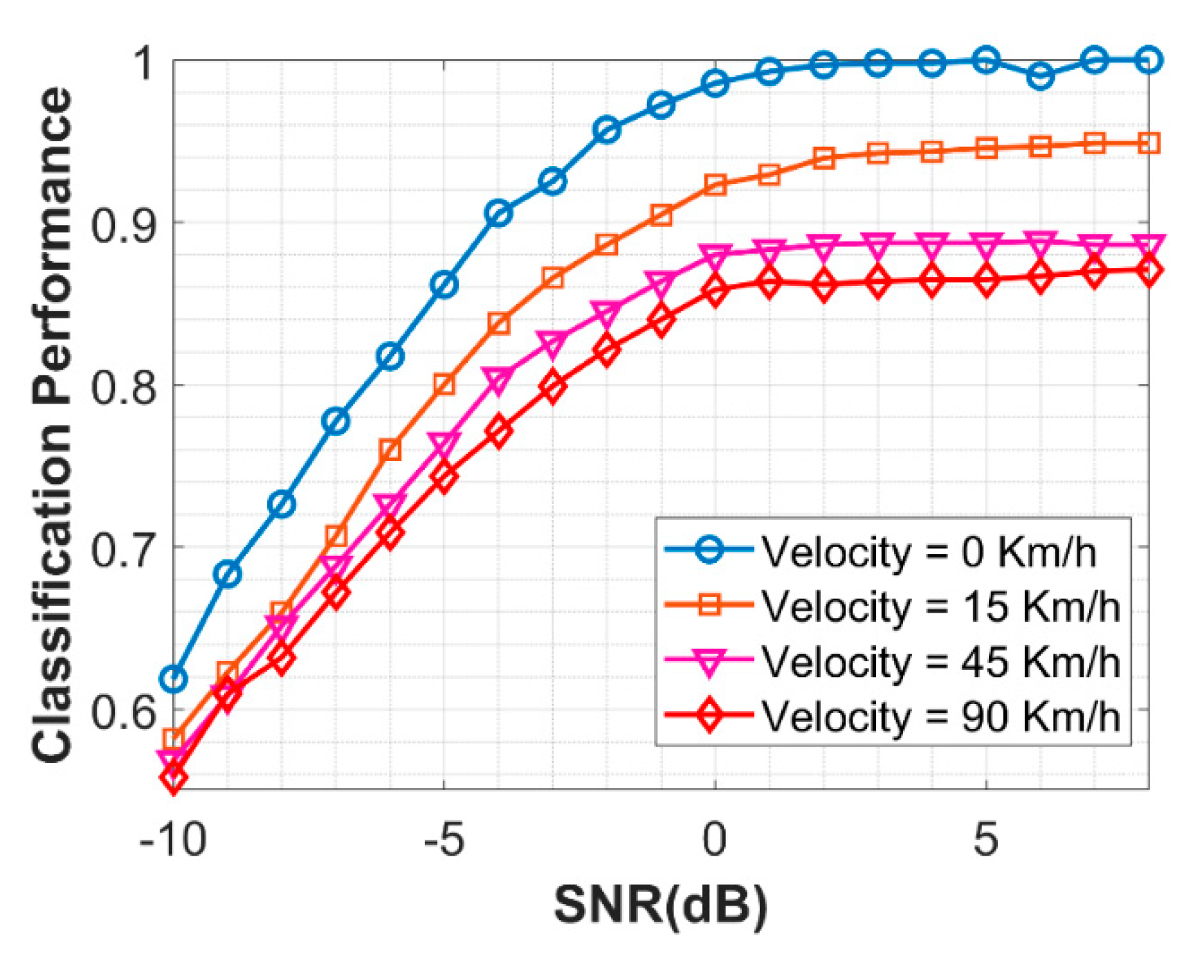
Effect of Velocity: In the real world, the signal is highly distorted due to small scale fading effects such as, multipath fading, scattering and Doppler shifts. Here, the performance of NSVM is observed under different Doppler shifts. The algorithm performance degrades with the increase in the Doppler shift caused by high velocity, which is given by Figure 13. Therefore, to overcome this, similarly to countering carrier frequency, offset can be used.

4.6. Comparative Study of Related Works

In this section, the performance of previous reported wireless signal classification algorithms at specific values of signal-to-noise ratio (SNR) are summarized and compared with NSVM. The analytical analysis performed in this section is given in Table 4, which shows that the proposed scheme NSVM achieves higher performance than its counterpart in both low and high SNR scenarios.

5. Conclusions

In this paper, a novel feature-based classifier NSVM has been proposed for Automatic Classification of Wireless Signals, in which the features were learned automatically from raw input signals by using Convolutional Neural Networks (CNN). The output of NSVM is given by a Gaussian Support Vector Machine (SVM), which takes the features learned by CNN as its input. Therefore, the proposed schemes NSVM learned to minimize a margin-based loss instead of a cross-entropy loss. The proposed scheme outperformed the traditional softmax-based CNN classifier by achieving faster convergence of accuracy and loss curves during training/validation. Furthermore, the robustness of the NSVM classifier was verified by extensive simulation experiments under the presence of several non-ideal real-world channel impairments over a range of signal-to-noise values. The performance of the NSVM was remarkable in classifying wireless signals, for example, at a low signal-to-noise ratio (SNR), the overall averaged classification accuracy was >97% at SNR = −2 dB, and at a high SNR, it achieved an overall classification accuracy of >99% at SNR = 10 dB. In addition to that, in the analytical comparison with other studies, the results showed that the performance of NSVM is superior over a range of settings.
Although, the proposed approach may not always perform well for all modulations under different conditions, so there is still room for improvement. As NSVM is not dependent on N, a parallel computation can be introduced to train deeper models because the classifier performance is greatly dependent on the architecture and the depth of the feature extraction module. Extended implications of the proposed scheme also include increasing the number of modulation schemes to classify.

Author Contributions

Conceptualization, A.H.W. and Y.W.; methodology, A.H.W. and Y.W.; validation, A.H.W., Y.W. and R.C.; writing, review and editing, A.H.W. and Y.W.; funding acquisition, L.C.

Funding

This work was support in part by National Science and Technology under grant 2016ZX03002003-003 and in part by the Beijing Science and Technology project under grant Z171100001117147.

Acknowledgments

The first Author, A.H.W., hereby acknowledges the University of Chinese Academy of Science (CAS) and The World Academy of Sciences (TWAS) for financial support of Ph.D. studies under the CAS-TWAS Fellowship.

Conflicts of Interest

The authors declare no conflict of interest.

References

  1. Qian, G.; Ruan, Z.; Lu, J. Joint modulation classification and user number detection for multiuser MIMO-STBC systems. Information 2016, 7, 70. [Google Scholar] [CrossRef]
  2. Dobre, O.A.; Abdi, A.; Bar-Ness, Y.; Su, W. Survey of automatic modulation classification techniques: Classical approaches and new trends. IET Commun. 2007, 1, 137–156. [Google Scholar] [CrossRef]
  3. Dobre, O.A.; Hameed, F. Likelihood-based algorithms for linear digital modulation classification in fading channels. In Proceedings of the 2006 Canadian Conference on Electrical and Computer Engineering, Ottawa, ON, Canada, 7–10 May 2006; pp. 1347–1350. [Google Scholar]
  4. Panagiotou, P.; Anastasopoulos, A.; Polydoros, A. Likelihood ratio tests for modulation classification. In Proceedings of the MILCOM 2000 Proceedings. 21st Century Military Communications. Architectures and Technologies for Information Superiority (Cat. No. 00CH37155), Los Angeles, CA, USA, 22–25 October 2000; pp. 670–674. [Google Scholar]
  5. Xu, J.L.; Su, W.; Zhou, M. Likelihood-ratio approaches to automatic modulation classification. IEEE Trans. Syst. Man Cybern. Part C Appl. Rev. 2010, 41, 455–469. [Google Scholar] [CrossRef]
  6. Azzouz, E.E.; Nandi, A.K. Automatic identification of digital modulation types. Signal Process. 1995, 47, 55–69. [Google Scholar] [CrossRef]
  7. Swami, A.; Sadler, B.M. Hierarchical digital modulation classification using cumulants. IEEE Trans. Commun. 2000, 48, 416–429. [Google Scholar] [CrossRef]
  8. Wang, Y.-E.; Zhang, T.-Q.; Bai, J.; Bao, R. Modulation recognition algorithms for communication signals based on particle swarm optimization and support vector machines. In Proceedings of the 2011 Seventh International Conference on Intelligent Information Hiding and Multimedia Signal Processing, Dalian, China, 14–16 October 2011; pp. 266–269. [Google Scholar]
  9. Yu, Z. Automatic Modulation Classification of Communication Signals. New Jersey Institute of Technology 2006. Available online: https://digitalcommons.njit.edu/cgi/viewcontent.cgi?article=1848&context=dissertations (accessed on 30 October 2019).
  10. Zhu, Z.; Nandi, A.K. Automatic Modulation Classification: Principles, Algorithms and Applications; John Wiley & Sons: Hoboken, NJ, USA, 2015. [Google Scholar]
  11. Gang, H.; Jiandong, L.; Donghua, L. Study of modulation recognition based on HOCs and SVM. In Proceedings of the 2004 IEEE 59th Vehicular Technology Conference, VTC 2004-Spring (IEEE Cat. No. 04CH37514), Milan, Italy, 17–19 May 2004; pp. 898–902. [Google Scholar]
  12. Aslam, M.W.; Zhu, Z.; Nandi, A.K. Automatic modulation classification using combination of genetic programming and KNN. IEEE Trans. Wirel. Commun. 2012, 11, 2742–2750. [Google Scholar]
  13. Berman, D.S.; Buczak, A.L.; Chavis, J.S.; Corbett, C.L. A survey of deep learning methods for cyber security. Information 2019, 10, 122. [Google Scholar] [CrossRef]
  14. LeCun, Y.; Bengio, Y.; Hinton, G. Deep learning. Nature 2015, 521, 436–444. [Google Scholar] [CrossRef] [PubMed]
  15. Jarrett, K.; Kavukcuoglu, K.; Ranzato, M.A.; LeCun, Y. What is the best multi-stage architecture for object recognition? In Proceedings of the 2009 IEEE 12th International Conference on Computer Vision, Kyoto, Japan, 29 September–2 October 2009; pp. 2146–2153. [Google Scholar]
  16. Krizhevsky, A.; Sutskever, I.; Hinton, G.E. Imagenet classification with deep convolutional neural networks. In Proceedings of the Advances in Neural Information Processing Systems, Lake Tahoe, NV, USA, 3–8 December 2012; pp. 1097–1105. [Google Scholar]
  17. Jiao, Y.; Latifi, S.; Yang, M. Self error detection and correction for noisy labels based on error correcting output code in convolutional neural networks. In Proceedings of the 2019 IEEE 9th Annual Computing and Communication Workshop and Conference (CCWC 2019), Las Vegas, NV, USA, 7–9 January 2019; pp. 0311–0316. [Google Scholar]
  18. Dahl, G.E.; Yu, D.; Deng, L.; Acero, A. Context-dependent pre-trained deep neural networks for large-vocabulary speech recognition. IEEE Trans. Audio Speech Lang. Process. 2011, 20, 30–42. [Google Scholar] [CrossRef]
  19. Wallach, I.; Dzamba, M.; Heifets, A. AtomNet: A deep convolutional neural network for bioactivity prediction in structure-based drug discovery. arXiv 2015, arXiv:1510.02855. [Google Scholar]
  20. Amato, F.; Marrone, S.; Moscato, V.; Piantadosi, G.; Picariello, A.; Sansone, C. HOLMeS: Ehealth in the big data and deep learning era. Information 2019, 10, 34. [Google Scholar] [CrossRef]
  21. O’Shea, T.J.; Roy, T.; Clancy, T.C. Over-the-air deep learning based radio signal classification. IEEE J. Sel. Top. Signal Process. 2018, 12, 168–179. [Google Scholar] [CrossRef]
  22. O’Shea, T.; Hoydis, J. An introduction to deep learning for the physical layer. IEEE Trans. Cogn. Commun. Netw. 2017, 3, 563–575. [Google Scholar] [CrossRef]
  23. Li, M.; Li, O.; Liu, G.; Zhang, C. Generative adversarial networks-based semi-supervised automatic modulation recognition for cognitive radio networks. Sensors 2018, 18, 3913. [Google Scholar] [CrossRef] [PubMed]
  24. Wang, H.; Wu, Z.; Ma, S.; Lu, S.; Zhang, H.; Ding, G.; Li, S. Deep learning for signal demodulation in physical layer wireless communications: Prototype platform, open dataset, and analytics. IEEE Access 2019, 7, 30792–30801. [Google Scholar] [CrossRef]
  25. Liang, Y.; Xiang, X.; Sun, Y.; Da, X.; Li, C.; Yin, L. Novel modulation recognition for WFRFT-based system using 4th-order cumulants. IEEE Access 2019, 7, 86018–86025. [Google Scholar] [CrossRef]
  26. Zhou, S.; Yin, Z.; Wu, Z.; Chen, Y.; Zhao, N.; Yang, Z. A robust modulation classification method using convolutional neural networks. EURASIP J. Adv. Signal Process. 2019, 2019, 21. [Google Scholar] [CrossRef] [Green Version]
  27. Boser, B.E.; Guyon, I.M.; Vapnik, V.N. A training algorithm for optimal margin classifiers. In Proceedings of the Proceedings of the Fifth Annual Workshop on Computational Learning Theory, Pittsburgh, PA, USA, 27–29 July 1992; pp. 144–152. [Google Scholar]
  28. Agarap, A.F. An architecture combining convolutional neural network (CNN) and support vector machine (SVM) for image classification. arXiv 2017, arXiv:1712.03541. [Google Scholar]
  29. Huang, F.-J.; LeCun, Y. Large-scale learning with svm and convolutional nets for generic object categorization. In Proceedings of the Proc. Computer Vision and Pattern Recognition Conference (CVPR’06), New York, NY, USA, 17–22 June 2006. [Google Scholar]
  30. LeCun, Y.; Bottou, L.; Bengio, Y.; Haffner, P. Gradient-based learning applied to document recognition. Proc. IEEE 1998, 86, 2278–2324. [Google Scholar] [CrossRef] [Green Version]
  31. Zhang, M.; Diao, M.; Guo, L. Convolutional neural networks for automatic cognitive radio waveform recognition. IEEE Access 2017, 5, 11074–11082. [Google Scholar] [CrossRef]
Figure 1. A simple block-wise architecture of a Feature-Based (FB) classifier.
Information 10 00338 g001
Figure 2. Convolutional Neural Networks (CNN).
Information 10 00338 g002
Figure 3. Support Vector Machine (SVM) separating the hyperplane for Binary Classification.
Information 10 00338 g003
Figure 4. Neural-Induced Support Vector Machine (NSVM) Architecture.
Information 10 00338 g004
Figure 5. Training and validation curves of accuracy and loss of NSVM classifier. The x-axis denotes the training epochs.
Information 10 00338 g005
Figure 6. Training and validation curves of accuracy and loss of the CNN model with the softmax classifier. The x-axis denotes the training epochs.
Information 10 00338 g006
Figure 7. The performance of NSVM for different individual modulation schemes.
Information 10 00338 g007
Figure 8. Performance of NSVM with different sampling points.
Information 10 00338 g008
Figure 9. Performance of NSVM for QAM16 and QAM64 with N = 1024, 2048 sampling points.
Information 10 00338 g009
Figure 10. Performance of NSVM with Different Carrier Frequency Offset in received signal.
Information 10 00338 g010
Figure 11. Performance of NSVM with different Phase Offsets.
Information 10 00338 g011
Figure 12. The Performance of NSVM with Different Timing Offsets.
Information 10 00338 g012
Figure 13. The Performance of NSVM with different Doppler Shifts relative to Velocity.
Information 10 00338 g013
Table 1. Dataset Parameters.
ParametersSymbolsValues
Carrier Frequency f c 10 MHz
Number of Samples per input frameN2048
SNR −10 dB to 8 dB
Symbols per Frame N f 256
Samples per Symbol N s 8
Table 2. Confusion Matrix of NSVM at SNR = −4 dB.
SNR = −4 dBTrue Class
Predicted Class BPSK4-ASKQPSK16-QAM64-QAM8-PSK
BPSK100
4-ASK 100
QPSK 91.18 8.82
16-QAM 79.907.6712.43
64-QAM 1.8398.17
8-PSK 18.8712.26 68.87
Table 3. Confusion Matrix of NSVM at SNR = 0 dB.
SNR = 0 dBTrue Class
Predicted Class BPSK4-ASKQPSK16-QAM64-QAM8-PSK
BPSK100
4-ASK 100
QPSK 95.57 2.43
16-QAM 94.491.284.23
64-QAM 0.5499.46
8-PSK 5.870.85 93.28
Table 4. Comparison with other works.
ClassifierModulationsSNRAccuracy
Artificial Neural Networks Based on spectral features [6]
NSVM
BPSK, QPSK, 8PSK, QAM16,
QAM 64
−5 dB
−5 dB
83.7%
86.3%
Deep BeliefNetworks (DBN)-SVM [24],
KNNAdaBoost [24]
NSVM
BPSK, QPSK, QAM16, QAM 648 dB
8 dB
8 dB
75.5%
89.9%
99.8%
Convolution Neural Networks [31]
NSVM
2FSK, DQPSK, 16AM, MSK, GMSK0 dB
0 dB
83.5%
98.2%
GPKNN [12]
NSVM
BPSK, QPSK, QAM16, QAM 6410 dB
10 dB
97%
99.9%
Convolutional Neural Networks with Cumulants [25]
NSVM
BPSK, QPSK, 8PSK, 4ASK, QAM16, QAM 646 dB
6 dB
90%
99%