Abstract
Diagnosability of a multiprocessor system is an important topic of study. A measure for fault diagnosis of the system restrains that every fault-free node has at least g fault-free neighbor vertices, which is called the g-good-neighbor diagnosability of the system. As a famous topology structure of interconnection networks, the n-dimensional bubble-sort graph has many good properties. In this paper, we prove that (1) the 1-good-neighbor diagnosability of is under Preparata, Metze, and Chien’s (PMC) model for and Maeng and Malek’s (MM) model for ; (2) the 2-good-neighbor diagnosability of is under the PMC model and the MM model for ; (3) the 3-good-neighbor diagnosability of is under the PMC model and the MM model for .
1. Introduction
A multiprocessor system and interconnection network (networks for short) have an underlying topology, which is usually presented by a graph, where nodes represent processors and links represent communication links between processors. We use graphs and networks interchangeably. For the system, some processors may fail in the system, so processor fault identification plays an important role in reliable computing. The first step to deal with faults is to identify the faulty processors from the fault-free ones. The identification process is called the diagnosis of the system. A system is said to be t-diagnosable if all faulty processors can be identified without replacement, provided that the number of faulty processors presented does not exceed t. The diagnosability of a system G is the maximum value of t such that G is t-diagnosable. Several diagnosis models (e.g., Preparata, Metze, and Chien’s (PMC) model [1], Barsi, Grandoni, and Maestrini’s (BGM) model [2], and Maeng and Malek’s (MM) model [3]) have been proposed to investigate the diagnosability of multiprocessor systems. In particular, two of the proposed models, the PMC model and MM model, are well known and widely used. In the PMC model, the diagnosis of the system is achieved through two linked processors testing each other. In the MM model, to diagnose a system, a node sends the same task to two of its neighbor vertices, and then compares their responses. Sengupta and Dahbura [4] proposed a special case of the MM model, called the MM* model, in which each node must test all the pairs of its adjacent nodes. In 2012, Peng et al. [5] proposed a measure for fault diagnosis of the system, namely, the g-good-neighbor diagnosability of the system (which is also called g-good-neighbor conditional diagnosability), which requires that every fault-free node contains at least g fault-free neighbors. In [5], they studied the g-good-neighbor diagnosability of the n-dimensional hypercube under the PMC model. Numerous studies have been investigated under the PMC model and MM model or MM* model, see [1,2,3,4,5,6,7,8,9,10,11,12,13,14,15,16,17,18,19,20,21].
In this paper, we prove that (1) the diagnosability of n-dimensional bubble-sort graph is under the PMC model for ; (2) the 1-good-neighbor diagnosability of is under the PMC model for and the MM model for ; (3) the 2-good-neighbor diagnosability of is under the PMC model and the model for ; (4) the 3-good-neighbor diagnosability of is under the PMC model and the MM model for .
2. Preliminaries
In this section, some definitions and notations needed are introduced for our discussion, then bubble-sort graphs will be introduced.
2.1. Definitions and Notations
A multiprocessor system is modeled as an undirected simple graph , whose vertices (nodes) represent processors and edges (links) represent communication links. Given a nonempty vertex subset of V, the induced subgraph by in G, denoted by , is a graph, whose vertex set is and the edge set is the set of all the edges of G with both endpoints in . The degree of a vertex v is the number of edges incident with v. We denote by the minimum degrees of vertices of G. For any vertex v, we define the neighborhood of v in G to be the set of vertices adjacent to v. u is called a neighbor vertex or a neighbor of v for . Let . We use to denote the set . For neighborhoods and degrees, we will usually omit the subscript for the graph when no confusion arises. A graph G is said to be k-regular if for any vertex v, . A graph is bipartite if its vertex set can be partitioned into two subsets X and Y so that every edge has one end in X and one end in Y; such a partition is called a bipartition of the graph, and X and Y its parts. We denote a bipartite graph G with bipartition by . If is simple and every vertex in X is joined to every vertex in Y, then is called a complete bipartite graph, denoted by , where and . Let be a connected graph. The connectivity of a graph G is the minimum number of vertices whose removal results in a disconnected graph or only one vertex left. A fault set is called a g-good-neighbor faulty set if for every vertex v in . A g-good-neighbor cut of a graph G is a g-good-neighbor faulty set F such that is disconnected. The minimum cardinality of g-good-neighbor cuts is said to be the g-good-neighbor connectivity of G, denoted by . For graph-theoretical terminology and notation not defined here we follow [22].
2.2. The Bubble-Sort Graph
The bubble-sort graph has been known as a famous topology structure of interconnection networks. In this section, its definition and some useful properties are introduced.
In the permutation , . For the convenience, we denote the permutation by . Every permutation can be denoted by a product of cycles [23]. For example, . Specially, . The product of two permutations is the composition function followed by , for example, . For terminology and notation not defined here we follow [23].
Let , and let be the symmetric group on containing all permutations of . It is well known that is a generating set for . The n-dimensional bubble-sort graph [24] is the graph with vertex set = in which two vertices u, v are adjacent if and only if , . It is easy to see from the definition that is a -regular graph on vertices. The graphs , and are depicted in Figure 1.
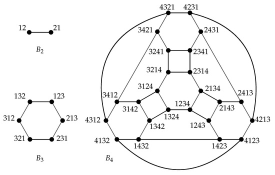
Figure 1.
The bubble-sort graphs , and .
Note that is a subclass of Cayley graphs. has the following useful properties.
Proposition 1.
For any integer , is -regular and vertex transitive.
Proposition 2.
For any integer , is bipartite.
Proposition 3.
For any integer , the girth of is 4.
Theorem 1
([23]). Every nonidentity permutation in the symmetric group is uniquely (up to the order of the factors) a product of disjoint cycles, each of which has length of at least 2.
Proposition 4
([12]). Let be a bubble-sort graph. If two vertices are adjacent, there is no common neighbor vertex of these two vertices, i.e., . If two vertices are not adjacent, there is at most two common neighbor vertices of these two vertices, i.e., .
Theorem 2
([7,25,26]). for .
Theorem 3
([7,25,26]). for .
Theorem 4
([7,25,26]). for .
Theorem 5
([27]). for and for .
3. The Diagnosability of the Bubble-Sort Graph under the PMC Model
In this section, we shall show the g-good-neighbor diagnosability of the bubble-sort graph under the PMC model for .
Let and be two distinct subsets of V for a system . Define the symmetric difference . Yuan et al. [20] presented a sufficient and necessary condition for a system to be g-good-neighbor t-diagnosable under the PMC model.
Lemma 1
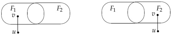
([20]). A system is g-good-neighbor t-diagnosable under the model if and only if there is an edge with and for each distinct pair of g-good-neighbor faulty subsets and of V with and (See Figure 2). The g-good-neighbor diagnosability of G is the maximum value of t such that G is g-good-neighbor t-diagnosable under the PMC model.
Figure 2.
Illustration of a distinguishable pair under Preparata, Metze, and Chien’s (PMC) model.
Theorem 6.
The diagnosability of the bubble-sort graph is under the PMC model when .
Proof.
Let . Then . Let and . Then and . Since and , there is no edge of between and . By Lemma 1, we show that is not n-diagnosable under the PMC model. Hence, by the definition of the diagnosability, we have that the diagnosability of is less than n-diagnosable, i.e., .
By the definition of the diagnosability, it is sufficient to show that is -diagnosable under the PMC model. By Lemma 1, to prove that is -diagnosable, it is equivalent to prove that there is an edge with and for each distinct pair of faulty subsets and of with and . We prove this statement by contradiction. Suppose that there are two distinct faulty subsets and of with and , but the vertex set pair is not satisfied with the condition in Theorem 1, i.e., there are no edges between and . Without loss of generality, assume that . Suppose . By the definition of , . It is obvious that for . Since , we have that , a contradiction. Therefore, . Since there are no edges between and , and and , we have that is a cut set. By Theorem 2, . Therefore, , which contradicts with that . So is -diagnosable. By the definition of , the diagnosability . □
Theorem 7.
The 1-good-neighbor diagnosability of is under the PMC model when .
Proof.
Let . By Proposition 2, . Let and . Then and . Let . By Proposition 4, and . By Proposition 2, and or and . Therefore, () in and is a 1-good-neighbor cut of . Since and , there is no edge of between and . By Lemma 1, we show that is not 1-good-neighbor -diagnosable under the PMC model. Hence, by the definition of the 1-good-neighbor diagnosability, we have that .
By the definition of the 1-good-neighbor diagnosability, it is sufficient to show that is 1-good-neighbor -diagnosable. By Lemma 1, to prove that is 1-good-neighbor -diagnosable, it is equivalent to prove that there is an edge with and for each distinct pair of 1-good-neighbor faulty subsets and of with and .
We prove this statement by contradiction. Suppose that there are two distinct 1-good-neighbor faulty subsets and of with and , but the vertex set pair is not satisfied with the condition in Lemma 1, i.e., there are no edges between and . Without loss of generality, assume that . Suppose . Since , we have that , a contradiction. Therefore, .
Since there are no edges between and , and is a 1-good-neighbor faulty set, has two parts and (for convenience). Thus, and . Similarly, when . Therefore, is also a 1-good-neighbor faulty set. When , is also a 1-good-neighbor faulty set. Since there are no edges between and , is a 1-good-neighbor cut. By Theorem 3, . Note that . Therefore, , which contradicts with that . So is 1-good-neighbor -diagnosable. By the definition of , . □
Lemma 2.
Let . If , , , then , , , and .
Proof.
By , we have that is a 4-cycle. By Propositions 3 and 4, . Thus from calculating, we have , .
Let and and . Let and . By Proposition 1, let . Then . By Proposition 2, there is no such that . Therefore, we consider only . We discuss the following cases.
Case 1. and , .
If , then a contradiction to . Therefore, . In this case, . Consider and , . Suppose . Since , . If , then . If , then, in , . If , then, in , . If , then . If , then, in , . If , then, or in , . Therefore, .
Case 2. and , .
Without loss of generality, let . Let . Then , . If , then . Note . Then . Suppose . Consider and , . If , then, by Theorem 1, . If , then . If , then, in , . If , then, or in , . If , then . If , then, in , . If , then, or in , . Therefore, .
By Cases 1 and 2, () in and is a 2-good-neighbor cut of . When , it is easy to verify that is a 2-good-neighbor cut of . □
Lemma 3.
Let . Then the 2-good-neighbor diagnosability under the PMC model.
Proof.
Let A be defined in Lemma 2, and let , . By Lemma 2, , , and . Therefore, and are both 2-good-neighbor faulty sets of with and . Since and , there is no edge of between and . By Lemma 1, we show that is not 2-good-neighbor -diagnosable under the PMC model. Hence, by the definition of 2-good-neighbor diagnosability, we conclude that the 2-good-neighbor diagnosability of is less than , i.e., . □
Lemma 4.
Let H be a subgraph of such that . Then .
By the definition of , we have Lemma 4.
Lemma 5.
Let . Then the 2-good-neighbor diagnosability under the PMC model.
Proof.
By the definition of 2-good-neighbor diagnosability, it is sufficient to show that is 2-good-neighbor -diagnosable. By Theorem 1, to prove is 2-good-neighbor -diagnosable, it is equivalent to prove that there is an edge with and for each distinct pair of 2-good-neighbor faulty subsets and of with and .
We prove this statement by contradiction. Suppose that there are two distinct 2-good-neighbor faulty subsets and of with and , but the vertex set pair is not satisfied with the condition in Lemma 1, i.e., there are no edges between and . Without loss of generality, assume that . Suppose . By the definition of , . It is obvious that for . Since , we have that , a contradiction. Therefore, .
Since there are no edges between and , and is a 2-good-neighbor faulty set, has two parts and . Thus, and . Similarly, when . Therefore, is also a 2-good-neighbor faulty set. When , is also a 2-good-neighbor faulty set. Since there are no edges between and , is a 2-good-neighbor cut. Since , by Theorem 4, . By Lemma 4, . Therefore, , which contradicts with that . So is 2-good-neighbor -diagnosable. By the definition of , . □
Combining Lemmas 3 and 5, we have the following theorem.
Theorem 8.
Let . Then the 2-good-neighbor diagnosability of the bubble-sort graph under the PMC model is .
Lemma 6.
Let . If , , , then , , and .
Proof.
By , we have that is 3-regular and .
Claim 1. for .
By Proposition 1, let . By Proposition 2, we consider only . Since , by Proposition 4, we have . The proof of Claim 1 is complete.
By Claim 1, . Thus from calculating, we have , . Let and and . Let and . By Proposition 1, let . Then . By Proposition 2, there is no such that . Therefore, we consider only .
Claim 2. .
Let . We discuss the following cases.
Case 1. and , .
If , then a contradiction to . Therefore, . Consider . If , then . Let .
Consider and , . Suppose . Since , . If , then . If , then, in , . If , then, in , . If , then . If , then, in , . If , then, or in , .
Consider and , . Suppose . Since , . If , then . If , then or in , . If , then or or (). When , in , . When , or in , . When , or in , .
Similarly, consider and . We have . Therefore, .
Case 2. and , .
Without loss of generality, let . Let . Then , . If , then . Note . Then . Suppose . Consider and , . If , then, by Theorem 1, . If , then . If , then, in , . If , then, or in , . If , then . If , then, or in , . If , then, or in , .
Consider and , . If , then, by Theorem 1, . If , then . If , then, in , . If , then, or in , . If , then . If , then, or in , . If , then, or in , . If , then . If , then, or in , . If , then, or in , .
Similarly, consider and . We have . Therefore, . The proof of Claim 2 is complete.
By Claim 2, () in and is a 3-good-neighbor cut of . □
Lemma 7.
Let . Then the 3-good-neighbor diagnosability under the PMC model.
Proof.
Let A be defined in Lemma 6, and let , . By Lemma 6, , , and . Therefore, and are both 3-good-neighbor faulty sets of with and . Since and , there is no edge of between and . By Lemma 1, we can deduce that is not 3-good-neighbor -diagnosable under the PMC model. Hence, by the definition of 3-good-neighbor diagnosability, we conclude that the 2-good-neighbor diagnosability of is less than , i.e., . □
Lemma 8.
Let H be a subgraph of such that . Then .
Proof.
Note that there is no subgraph of . Suppose, on the contrary, that there is a subgraph of such that and . Since is bipartite, let and , . By Proposition 1, let and . Since , , a contradiction to Proposition 4. Therefore, . □
Lemma 9.
Let . Then the 3-good-neighbor diagnosability under the PMC model.
Proof.
By the definition of 3-good-neighbor diagnosability, it is sufficient to show that is 3-good-neighbor -diagnosable. By Lemma 1, to prove is 3-good-neighbor -diagnosable, it is equivalent to prove that there is an edge with and for each distinct pair of 3-good-neighbor faulty subsets and of with and .
We prove this statement by contradiction. Suppose that there are two distinct 3-good-neighbor faulty subsets and of with and , but the vertex set pair is not satisfied with the condition in Lemma 1, i.e., there are no edges between and . Without loss of generality, assume that . Suppose . By the definition of , . It is obvious that for . Since , we have that , a contradiction. Therefore, .
Since there are no edges between and , and is a 3-good-neighbor faulty set, has two parts and . Thus, and . Similarly, when . Therefore, is also a 3-good-neighbor faulty set. When , is also a 3-good-neighbor faulty set. Since there are no edges between and , is a 3-good-neighbor cut. Since , by Theorem 5, . By Lemma 8, . Therefore, , which contradicts with that . So is 3-good-neighbor -diagnosable. By the definition of , . □
Combining Lemmas 7 and 9, we have the following theorem.
Theorem 9.
Let . Then the 3-good-neighbor diagnosability of the bubble-sort graph under the PMC model is .
4. The Diagnosability of the Bubble-Sort Graph under the MM Model
Before discussing the diagnosability of the bubble-sort graph under the MM model, we first give an existing result.
Lemma 10
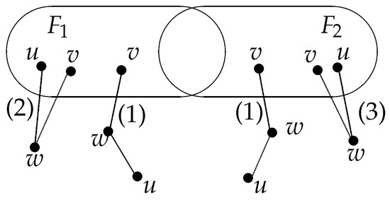
([4,20]). A system is g-good-neighbor t-diagnosable under the model if and only if for each distinct pair of g-good-neighbor faulty subsets and of V with and satisfies one of the following conditions. (1) There are two vertices and there is a vertex such that and . (2) There are two vertices and there is a vertex such that and . (3) There are two vertices and there is a vertex such that and (See Figure 3). The g-good-neighbor diagnosability of G is the maximum value of t such that G is g-good-neighbor t-diagnosable under the MM model.
Figure 3.
Illustration of a distinguishable pair under Maeng and Malek’s (MM)* model.
Theorem 10
([12]). The diagnosability of is under the MM model when .
A component of a graph G is odd according as it has an odd number of vertices. We denote by the number of odd component of G.
Lemma 11
([22]). A graph has a perfect matching if and only if for all .
Lemma 12
([22]). Let be an integer. Then every k-regular bipartite graph has k edge-disjoint perfect matchings.
Since the bubble-sort graph is a regular bipartite graph, we have the following corollary by Lemma 12.
Corollary 1.
The bubble-sort graph has a perfect matching.
Lemma 13.
Let . Then the 1-good-neighbor diagnosability of the bubble-sort graph under the MM model is less than or equal to , i.e., .
Proof.
Let and . Then u is adjacent to v. Let and . By Proposition 2, , . Let . By Proposition 4, and . By Proposition 2, if , then or if , then . Therefore, () in and is a 1-good-neighbor cut of . Since and , there is no edge of between and . By Lemma 10, we show that is not 1-good-neighbor -diagnosable under the MM model. Hence, by the definition of the 1-good-neighbor diagnosability, we have that . □
Lemma 14.
Let . Then the 1-good-neighbor diagnosability of the bubble-sort graph under the MM model is more than or equal to , i.e., .
Proof.
By the definition of 1-good-neighbor diagnosability, it is sufficient to show that is 1-good-neighbor -diagnosable. By Lemma 10, suppose, on the contrary, that there are two distinct 1-good-neighbor faulty subsets and of with and , but the vertex set pair is not satisfied with any one condition in Theorem 10. Without loss of generality, assume that Similarly to the discussion on in Theorem 3, we have .
Claim 1. has no isolated vertex.
Suppose, on the contrary, that has at least one isolated vertex w. Since is a 1-good-neighbor faulty set, there is a vertex such that u is adjacent to w. Since the vertex set pair is not satisfied with any one condition in Lemma 10, there is at most one vertex such that u is adjacent to w. Thus, there is just a vertex such that u is adjacent to w. Assume . Then . Since is a 1-good-neighbor faulty set, has no isolated vertex, a contradiction. Therefore, let as follows. Similarly, we can show that there is just a vertex such that v is adjacent to w. Let be the set of isolated vertices in , and let H be the subgraph induced by the vertex set . Then for any , there are neighbors in . By Corollary 1, has a perfect matching. By Lemma 11, . Assume . Note that . This is a contradiction to . So . Since the vertex set pair is not satisfied with the condition (1) of Theorem 10, and any vertex of is not isolated in H, we induce that there is no edge between and . Thus, is a vertex cut of and , i.e., is a 1-good-neighbor cut of . By Theorem 3, . Because and , and neither nor is empty, we have . Let and . Then for any vertex , w is adjacent to and . According to Proposition 4, there are at most three common neighbors for any pair of vertices in , it follows that there are at most two isolated vertices in , i.e., .
Suppose that there is exactly one isolated vertex v in . Let and be adjacent to v. Then . Note that has no 3-cycle. Thus, , , and and . Thus, . It follows that , which contradicts .
Suppose that there are exactly two isolated vertices v and w in . Let and be adjacent to v and w, respectively. Then , , , , and . , and . By Proposition 4, there are at most two common neighbors for any pair of vertices in . Thus, it follows that . Thus, . It follows that , which contradicts . The proof of Claim 1 is complete.
Let . By Claim 1, u has at least one neighbor in . Since the vertex set pair is not satisfied with any one condition in Lemma 10, by the condition (1) of Lemma 10, for any pair of adjacent vertices , there is no vertex such that and . It follows that u has no neighbor in . By the arbitrariness of u, there is no edge between and . Since and is a 1-good-neighbor faulty set, and hence . Since both and are 1-good-neighbor faulty sets, and there is no edge between and , is a 1-good-neighbor cut of . By Theorem 3, . Therefore, , which contradicts with that . So is 1-good-neighbor -diagnosable. By the definition of , . □
Combining Lemmas 13 and 14, we have the following theorem.
Theorem 11.
Let . Then the 1-good-neighbor diagnosability of the bubble-sort graph under the MM model is .
Lemma 15.
Let . Then the 2-good-neighbor diagnosability under the MM model.
Proof.
Let A, and be defined in Lemma 2. By the Lemma 2, , , then , , , and . So both and are 2-good-neighbor faulty sets. By the definitions of and , . Note , and . Therefore, both and are not satisfied with any one condition in Lemma 10, and is not 2-good-neighbor -diagnosable. Hence, . The proof is complete. □
Lemma 16.
Let . Then the 2-good-neighbor diagnosability under the MM model.
Proof.
By the definition of 2-good-neighbor diagnosability, it is sufficient to show that is 2-good-neighbor -diagnosable. By Lemma 10, suppose, on the contrary, that there are two distinct 2-good-neighbor faulty subsets and of with and , but the vertex set pair is not satisfied with any one condition in Lemma 10. Without loss of generality, assume that Similarly to the discussion on in Lemma 5, we have .
Claim 1. has no isolated vertex.
Suppose, on the contrary, that has at least one isolated vertex w. Since is a 2-good neighbor faulty set, there are two vertices such that u and v are adjacent to w. Since the vertex set pair is not satisfied with any one condition in Lemma 10, this is a contradiction. Therefore, has no isolated vertex. The proof of Claim 1 is complete.
Let . By Claim 1, u has at least one neighbor in . Since the vertex set pair is not satisfied with any one condition in Theorem 10, by the condition (1) of Lemma 10, for any pair of adjacent vertices , there is no vertex such that and . It follows that u has no neighbor in . By the arbitrariness of u, there is no edge between and . Since and is a 2-good-neighbor faulty set, . By Lemma 4, . Since both and are 2-good-neighbor faulty sets, and there is no edge between and , is a 2-good-neighbor cut of . By Theorem 4, we have . Therefore, , which contradicts . Therefore, is 2-good-neighbor -diagnosable and . The proof is complete. □
Combining Lemmas 15 and 16, we have the following theorem.
Theorem 12.
Let . Then the 2-good-neighbor diagnosability of the bubble-sort star graph under the model is .
We point out that is the least bubble-sort graph satisfying the three sufficient conditions in Lemma 10. Because is a cycle with six vertices which is isomorphic to the 3-dimensional star graph, by [21] is not 2-diagnosable.
Lemma 17.
Let . Then the 3-good-neighbor diagnosability under the MM model.
Proof.
Let A, and be defined in Lemma 6. By the Lemma 6, , , then , , , and . So both and are 3-good-neighbor faulty sets. By the definitions of and , . Note , and . Therefore, both and are not satisfied with any one condition in Lemma 10, and is not 3-good-neighbor -diagnosable. Hence, . The proof is complete. □
Lemma 18.
Let . Then the 3-good-neighbor diagnosability under the MM model.
Proof.
By the definition of 3-good-neighbor diagnosability, it is sufficient to show that is 3-good-neighbor -diagnosable. By Lemma 10, suppose, on the contrary, that there are two distinct 3-good-neighbor faulty subsets and of with and , but the vertex set pair is not satisfied with any one condition in Lemma 10. Without loss of generality, assume that Similarly to the discussion on in Lemma 9, we have .
Claim 1. has no isolated vertex.
Suppose, on the contrary, that has at least one isolated vertex w. Since is a 3-good neighbor faulty set, there are three vertices such that u, v and x are adjacent to w. Since the vertex set pair is not satisfied with any one condition in Lemma 10, this is a contradiction. Therefore, has no isolated vertex. The proof of Claim 1 is complete.
Let . By Claim 1, u has at least one neighbor in . Since the vertex set pair is not satisfied with any one condition in Theorem 10, by the condition (1) of Lemma 10, for any pair of adjacent vertices , there is no vertex such that and . It follows that u has no neighbor in . By the arbitrariness of u, there is no edge between and . Since and is a 3-good-neighbor faulty set, . By Lemma 8, . Since both and are 3-good-neighbor faulty sets, and there is no edge between and , is a 3-good-neighbor cut of . By Theorem 5, we have . Therefore, , which contradicts . Therefore, is 3-good-neighbor -diagnosable and . The proof is complete. □
Combining Lemmas 17 and 18, we have the following theorem.
Theorem 13.
Let . Then the 3-good-neighbor diagnosability of the bubble-sort graph under the model is .
5. Conclusions
In this paper, we investigate the problem of g-good-neighbor diagnosability of the n-dimensional bubble-sort graph under the PMC model and MM model and show g-good-neighbor diagnosability of is under the PMC model for and the MM model for , respectively.
The work will help engineers to develop more different networks.
Author Contributions
S.W. and Z.W. conceived and designed the study and wrote the manuscript. S.W. revised the manuscript. All authors read and approved the final manuscript.
Funding
This work is supported by the National Natural Science Foundation of China (61772010) and the Science Foundation of Henan Normal University (Xiao 20180529, 20180454).
Conflicts of Interest
The authors declare no conflict of interest.
References
- Preparata, F.P.; Metze, G.; Chien, R.T. On the connection assignment problem of diagnosable systems. IEEE Trans. Comput. 1967, 16, 848–854. [Google Scholar] [CrossRef]
- Barsi, F.; Grandoni, F.; Maestrini, P. A Theory of Diagnosability of Digital Systems. IEEE Trans. Comput. 1976, 25, 585–593. [Google Scholar] [CrossRef]
- Maeng, J.; Malek, M. A comparison connection assignment for self-diagnosis of multiprocessor systems. In Proceedings of the 11th International Symposium on Fault-Tolerant Computing, Portland, OR, USA, 24–26 June 1981; pp. 173–175. [Google Scholar]
- Dahbura, A.T.; Masson, G.M. An O(n2.5) Fault identification algorithm for diagnosable systems. IEEE Trans. Comput. 1984, 33, 486–492. [Google Scholar] [CrossRef]
- Peng, S.-L.; Lin, C.-K.; Tan, J.J.M.; Hsu, L.-H. The g-good-neighbor conditional diagnosability of hypercube under PMC model. Appl. Math. Comput. 2012, 218, 10406–10412. [Google Scholar] [CrossRef]
- Chang, N.-W.; Hsieh, S.-Y. Structural properties and conditional diagnosability of star graphs by using the PMC Model. IEEE Trans. Parallel Distrib. Syst. 2014, 25, 3002–3011. [Google Scholar] [CrossRef]
- Cheng, E.; Lipták, L. Fault resiliency of Cayley graphs generated by transpositions. Int. J. Found. Comput. Sci. 2007, 18, 1005–1022. [Google Scholar] [CrossRef]
- Fan, J. Diagnosability of crossed cubes under the comparison diagnosis model. IEEE Trans. Parallel Distrib. Syst. 2002, 13, 1099–1104. [Google Scholar]
- Hu, S.-C.; Yang, C.-B. Fault tolerance on star graphs. In Proceedings of the First Aizu International Symposium on Parallel Algorithms/Architecture Synthesis, Aizu-Wakamatsu, Japan, 15–17 March 1995; pp. 176–182. [Google Scholar]
- Lai, P.-L.; Tan, J.J.M.; Chang, C.-P.; Hsu, L.-H. Conditional diagnosability measures for large multiprocessor systems. IEEE Trans. Comput. 2005, 54, 165–175. [Google Scholar]
- Lin, C.-K.; Tan, J.J.M.; Hsu, L.-H.; Cheng, E.; Lipták, L. Conditional diagnosability of Cayley graphs generated by transposition trees under the comparison diagnosis Model. J. Interconnect. Netw. 2008, 9, 83–97. [Google Scholar] [CrossRef]
- Ren, Y.; Wang, S. Diagnosability of bubble-sort graph networks under the comparison diagnosis model. In Proceedings of the 2015 International Conference on Computational Intelligence and Communication Networks, Jabalpur, India, 12–14 December 2015; pp. 823–826. [Google Scholar]
- Wang, M.; Guo, Y.; Wang, S. The 1-good-neighbor diagnosability of Cayley graphs generated by transposition trees under the PMC model and MM* model. Int. J. Comput. Math. 2017, 94, 620–631. [Google Scholar] [CrossRef]
- Wang, M.; Lin, Y.; Wang, S. The 1-good-neighbor connectivity and diagnosability of Cayley graphs generated by complete graphs. Discret. Appl. Math. 2018, 246, 108–118. [Google Scholar] [CrossRef]
- Wang, M.; Lin, Y.; Wang, S. The connectivity and nature diagnosability of expanded k-ary n-cubes. RAIRO-Theor. Inform. Appl. 2017, 51, 71–89. [Google Scholar] [CrossRef]
- Wang, S.; Ren, Y. g-Good-neighbor diagnosability of arrangement graphs under the PMC model and MM* model. Information 2018, 9, 275. [Google Scholar] [CrossRef]
- Wang, S.; Zhao, L. A note on the nature diagnosability of alternating group graphs under the PMC model and MM* model. J. Interconnect. Netw. 2018, 18, 1850005. [Google Scholar] [CrossRef]
- Wang, S.; Wang, M. The g-good-neighbor and g-extra diagnosability of networks. Theor. Comput. Sci. 2018, in press. [Google Scholar] [CrossRef]
- Wang, S.; Han, W. The g-good-neighbor conditional diagnosability of n-dimensional hypercubes under the MM* model. Inf. Process. Lett. 2016, 116, 574–577. [Google Scholar] [CrossRef]
- Yuan, J.; Liu, A.; Ma, X.; Liu, X.; Qin, X.; Zhang, J. The g-good-neighbor conditional diagnosability of k-ary n-cubes under the PMC model and MM* model. IEEE Trans. Parallel Distrib. Syst. 2015, 26, 1165–1177. [Google Scholar] [CrossRef]
- Zheng, J.; Latifi, S.; Regentova, E.; Luo, K.; Wu, X. Diagnosability of star graphs under the comparison diagnosis Model. Inf. Process. Lett. 2005, 93, 29–36. [Google Scholar] [CrossRef]
- Bondy, J.A.; Murty, U.S.R. Graph Theory; Springer: New York, NY, USA, 2007. [Google Scholar]
- Hungerford, T.W. Algebra; Springer: New York, NY, USA, 1974. [Google Scholar]
- Akers, S.B. Balakrishnan Krishnamurthy, A group-theoretic model for symmetric interconnection networks. IEEE Trans. Comput. 1989, 38, 555–566. [Google Scholar] [CrossRef]
- Cheng, E.; Lipták, L.; Shawash, N. Orienting Cayley graphs generated by transposition trees. Comput. Math. Appl. 2008, 55, 2662–2672. [Google Scholar] [CrossRef]
- Yang, W.; Li, H.; Meng, J. Conditional connectivity of Cayley graphs generated by transposition trees. Inf. Process. Lett. 2010, 110, 1027–1030. [Google Scholar] [CrossRef]
- Shi, L.-S.; Wu, P. Conditional connectivity of bubble sort graphs. Acta Math. Appl. Sin. 2017, 33, 933–944. [Google Scholar] [CrossRef]


© 2019 by the authors. Licensee MDPI, Basel, Switzerland. This article is an open access article distributed under the terms and conditions of the Creative Commons Attribution (CC BY) license (http://creativecommons.org/licenses/by/4.0/).