Figure 1.
NB vs. Poisson models of exhortations (Paul).
Figure 1.
NB vs. Poisson models of exhortations (Paul).
Figure 2.
NB vs. Poisson models of imperatives (Paul).
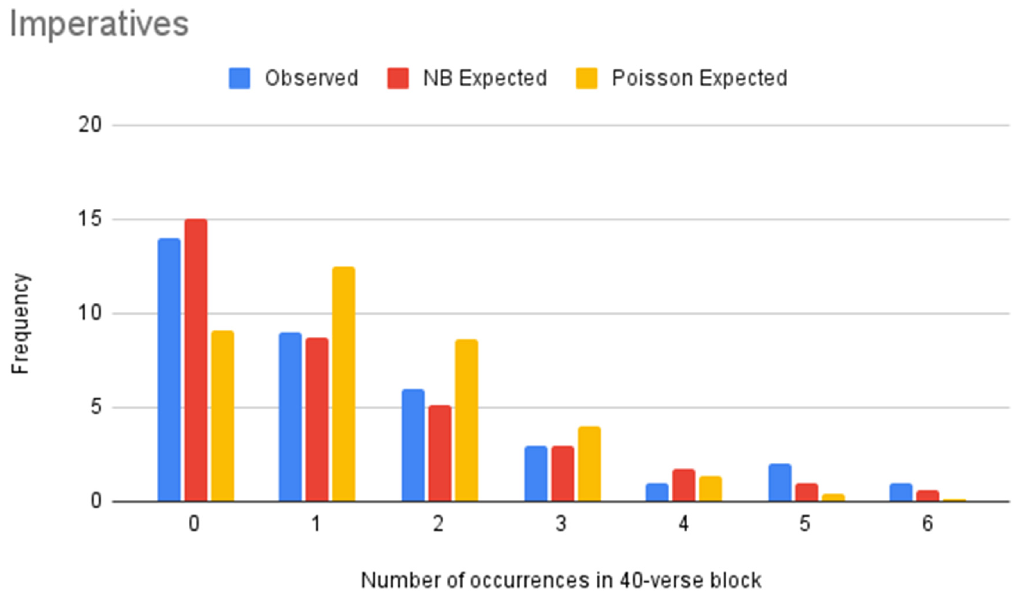
Figure 2.
NB vs. Poisson models of imperatives (Paul).
Figure 3.
NB vs. Poisson models of imperatives (Paul).
Figure 3.
NB vs. Poisson models of imperatives (Paul).
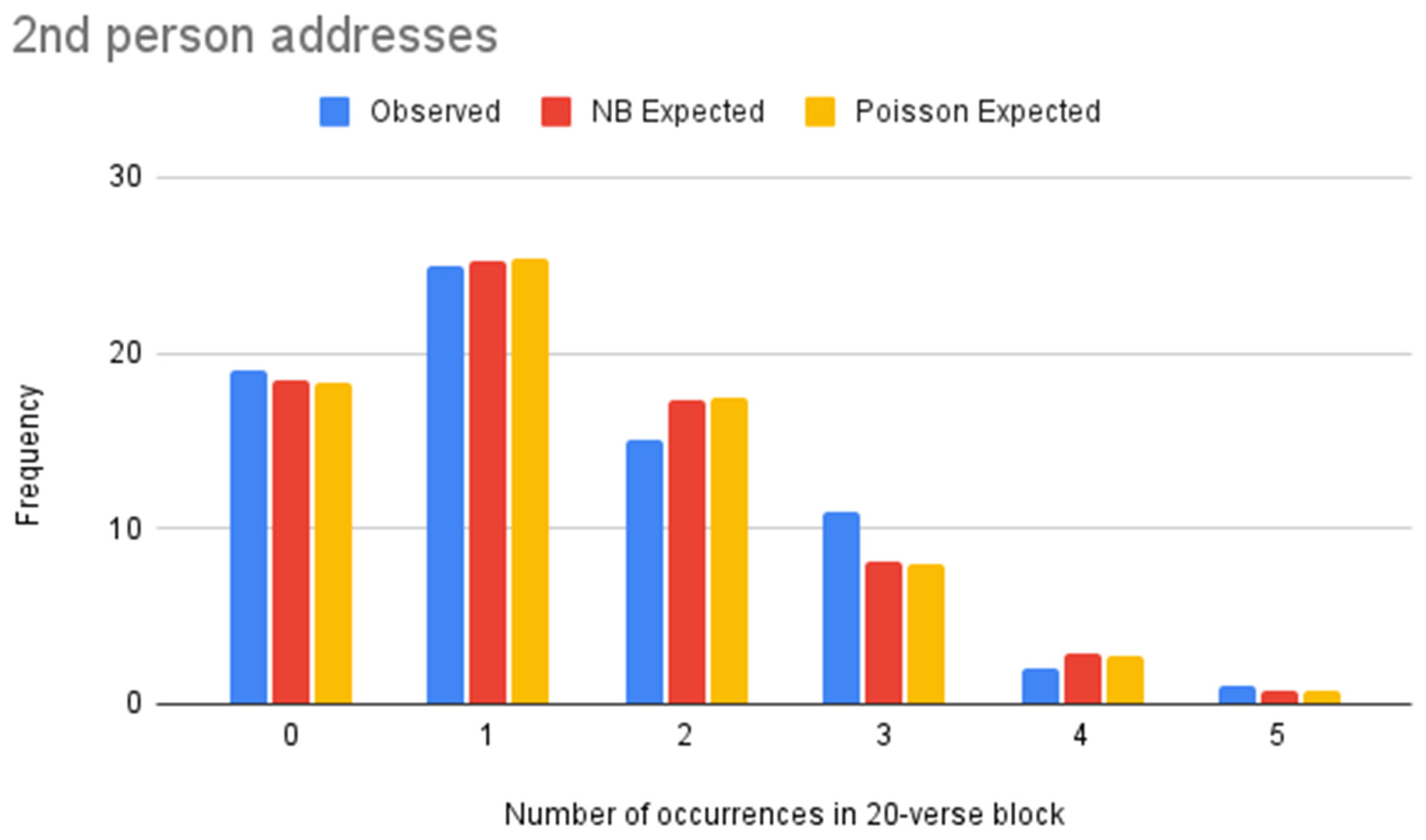
Figure 4.
NB vs. Poisson models for second person addresses (Paul).
Figure 4.
NB vs. Poisson models for second person addresses (Paul).
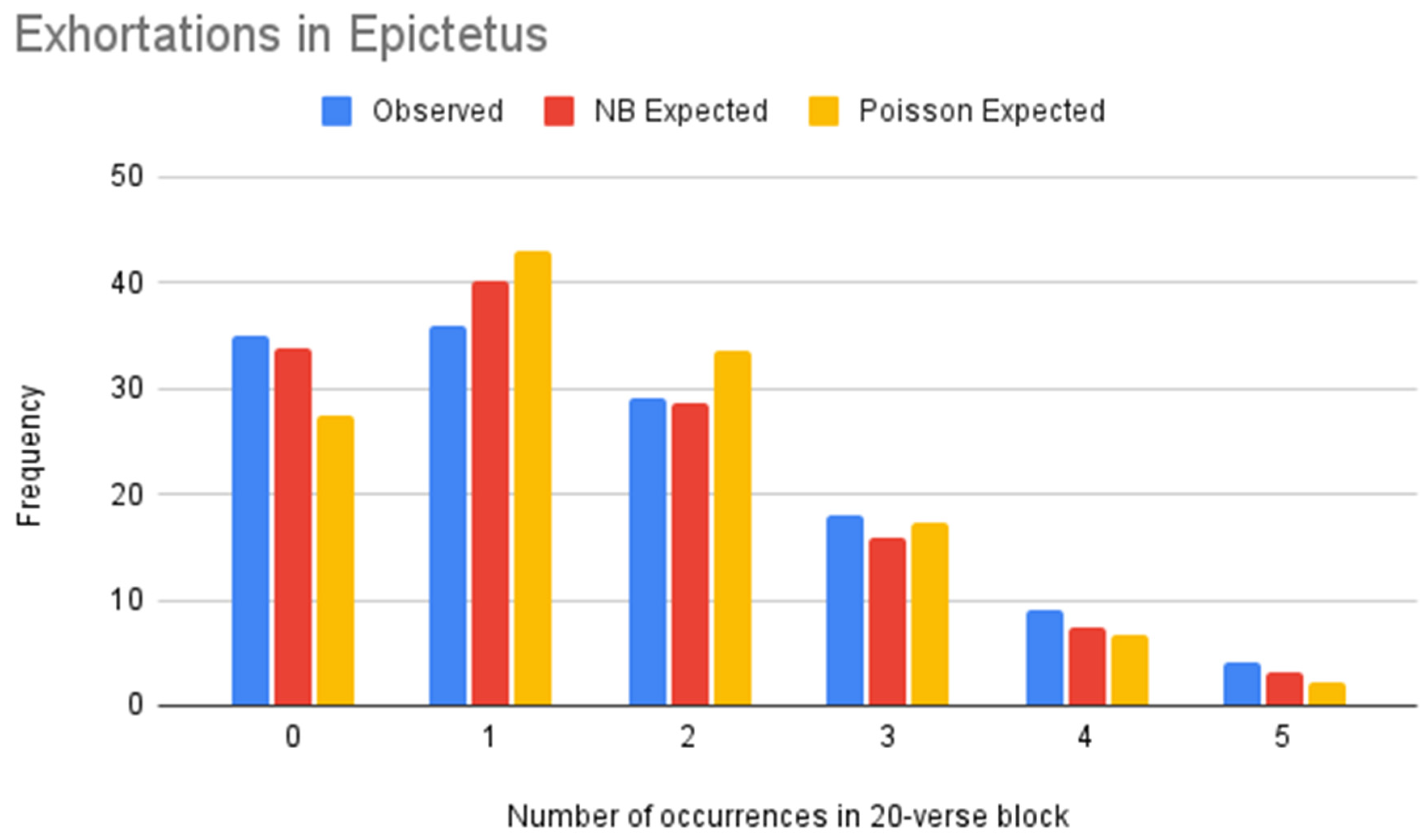
Figure 5.
NB vs. Poisson models of exhortations (Epictetus).
Figure 5.
NB vs. Poisson models of exhortations (Epictetus).
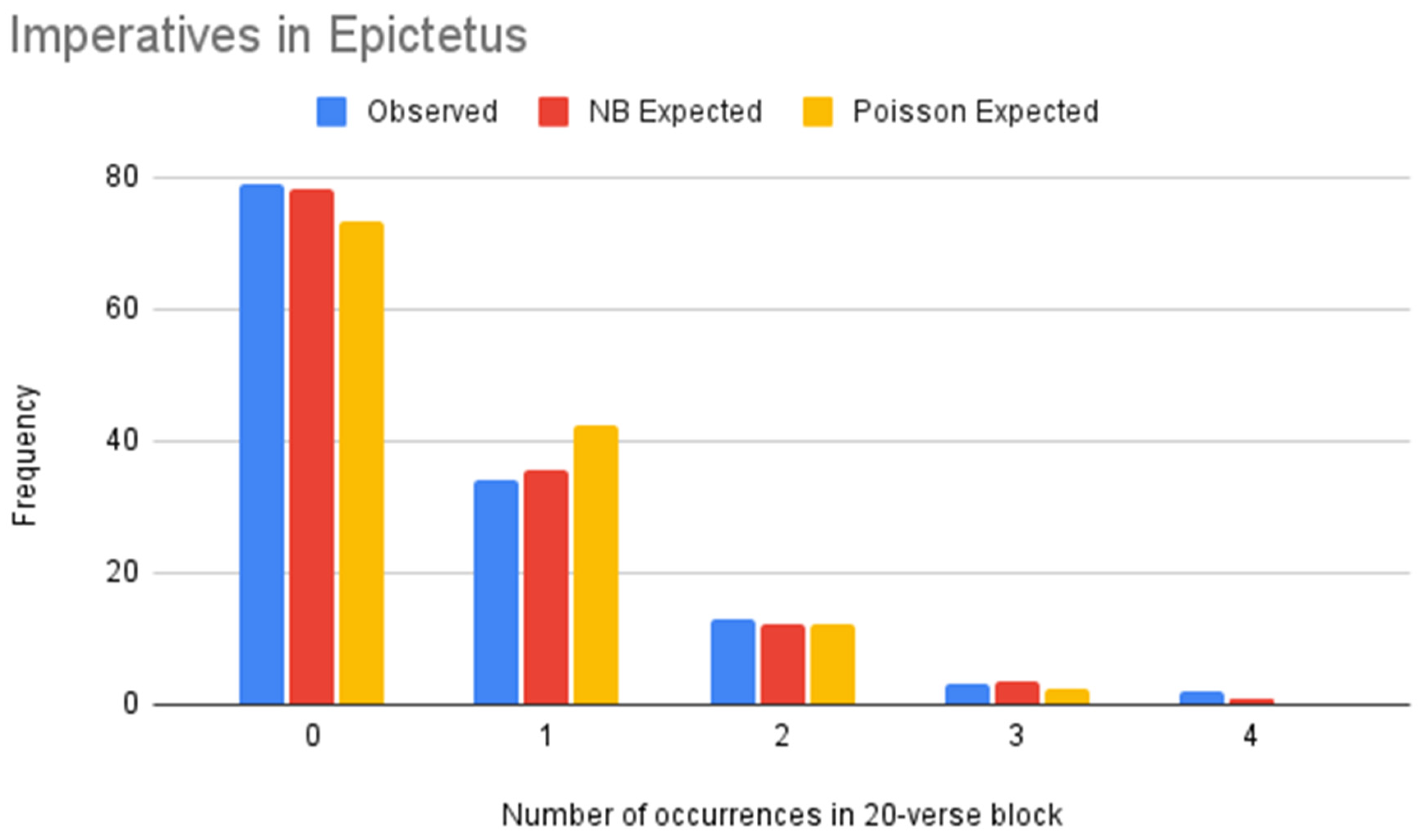
Figure 6.
NB vs. Poisson models of imperatives (Epictetus).
Figure 6.
NB vs. Poisson models of imperatives (Epictetus).
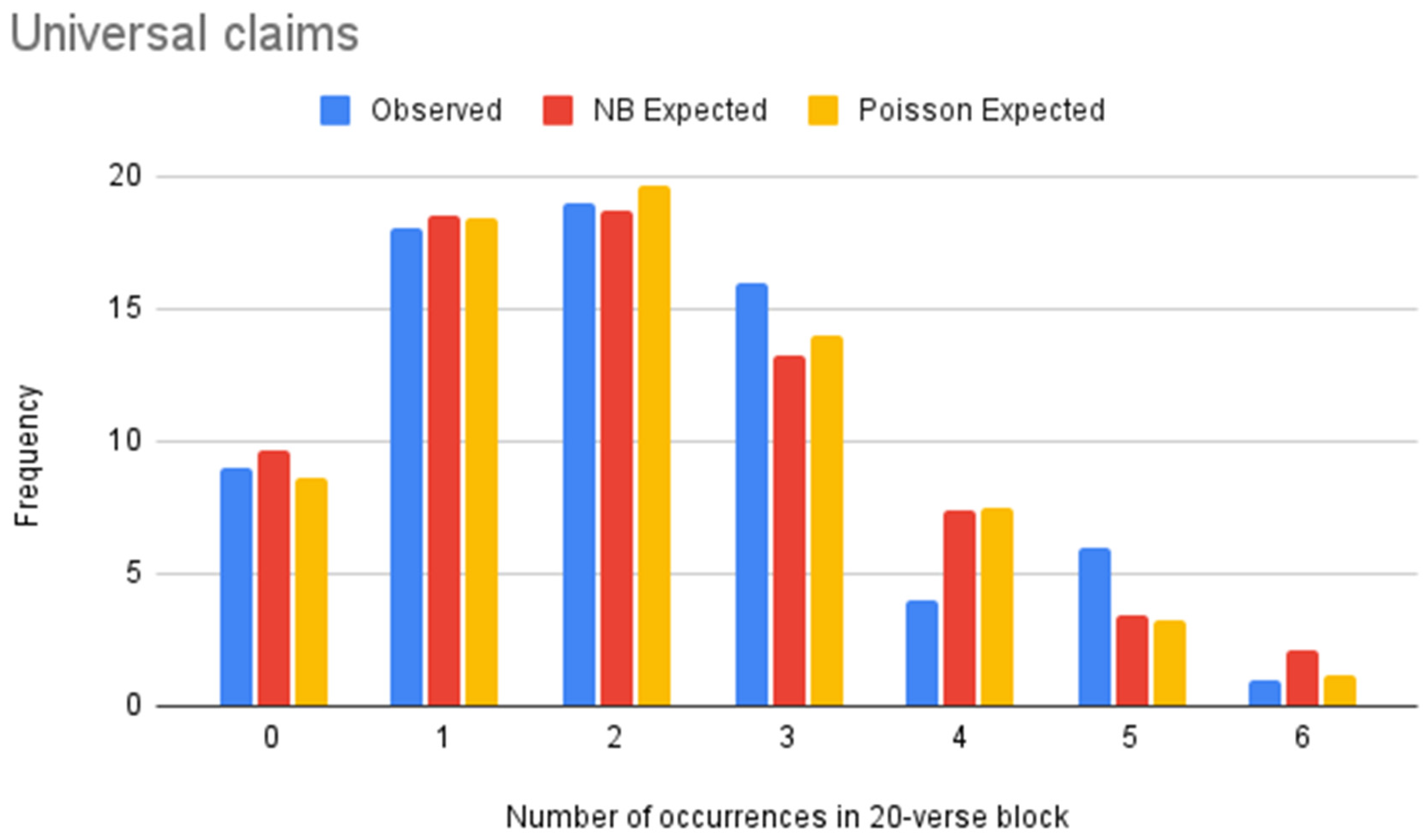
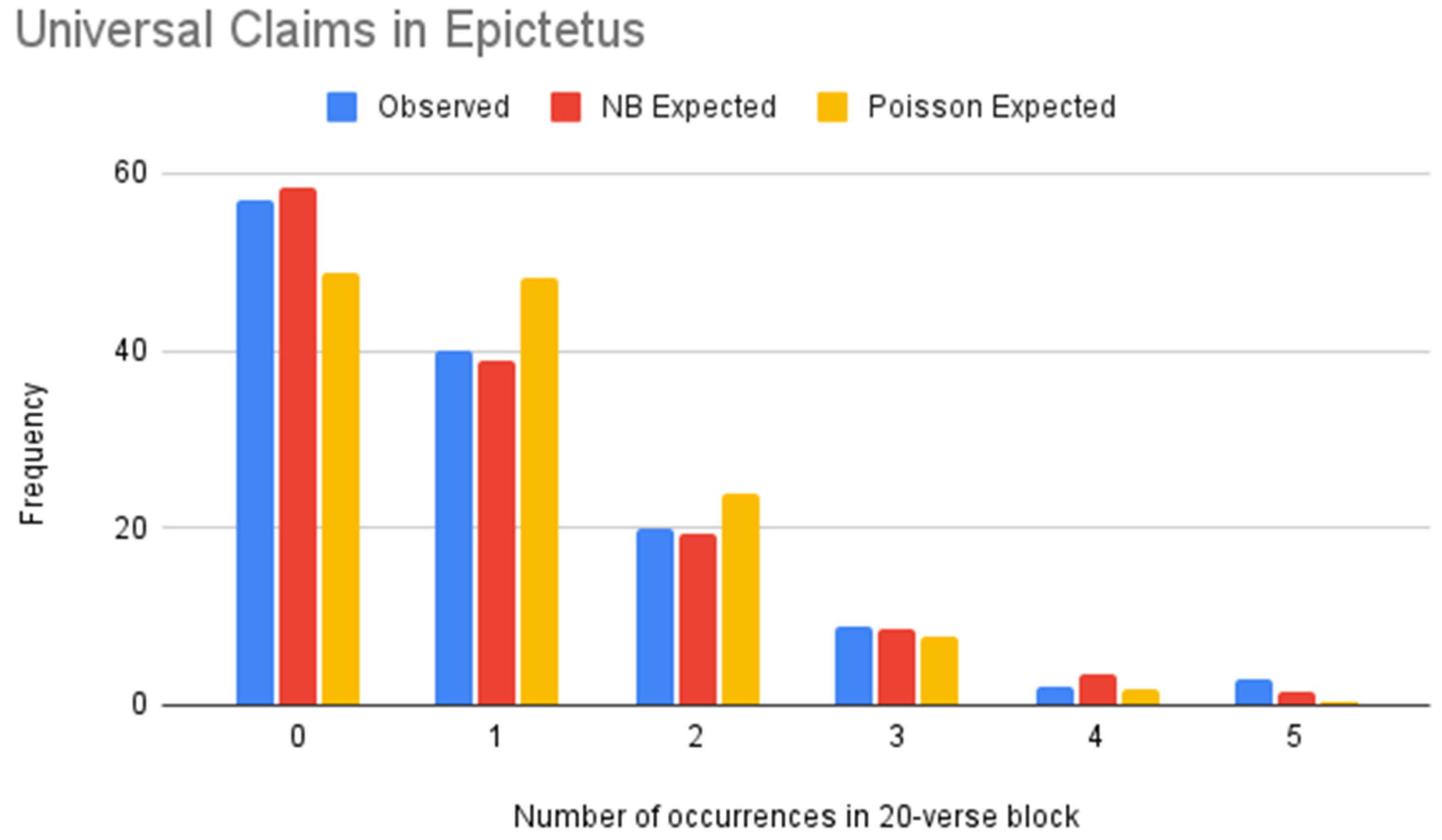
Figure 7.
NB vs. Poisson models of universal claims (Epictetus).
Figure 7.
NB vs. Poisson models of universal claims (Epictetus).
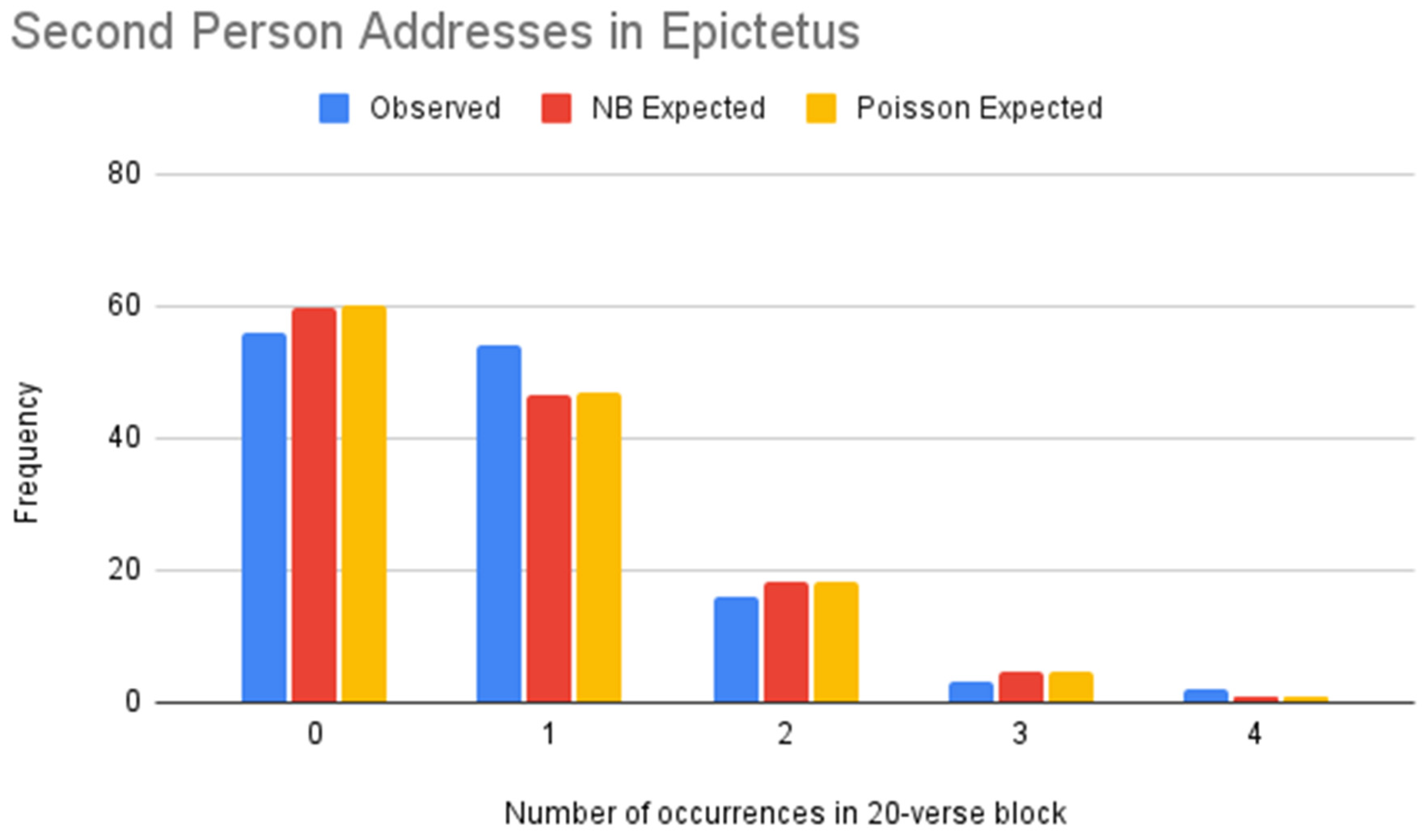
Figure 8.
NB vs. Poisson models of second person addresses (Epictetus).
Figure 8.
NB vs. Poisson models of second person addresses (Epictetus).
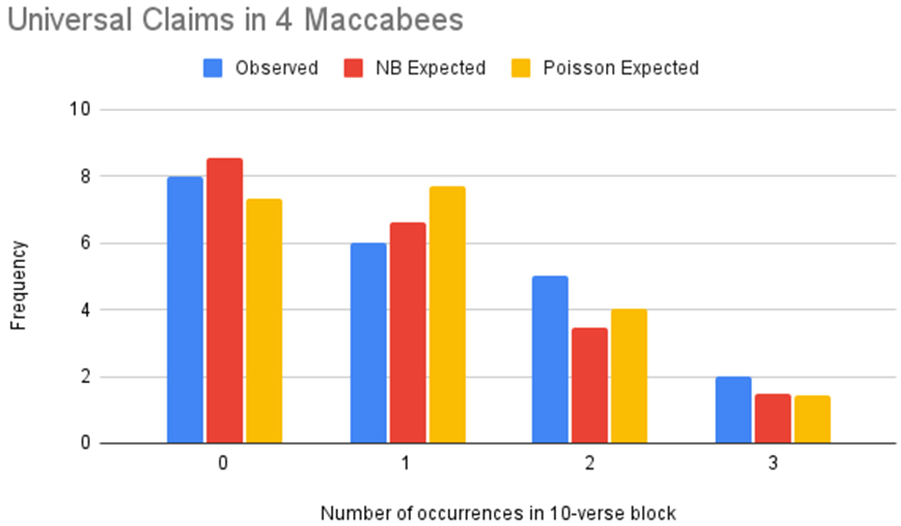
Figure 9.
NB vs. Poisson models of universal claims (4 Maccabees).
Figure 9.
NB vs. Poisson models of universal claims (4 Maccabees).
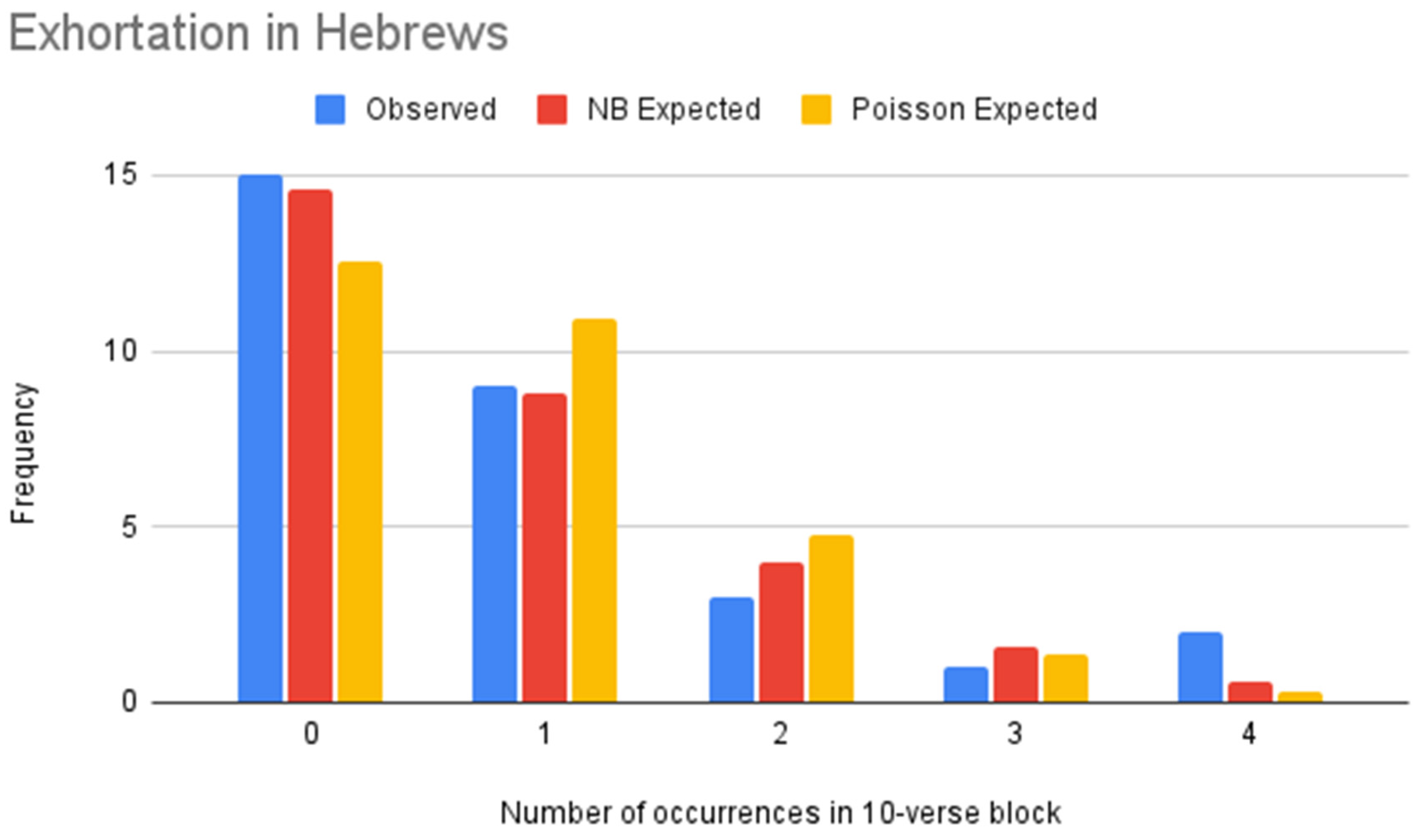
Figure 10.
NB vs. Poisson models of second person addresses (Hebrews).
Figure 10.
NB vs. Poisson models of second person addresses (Hebrews).
Figure 11.
NB vs. Poisson models of universal claims (Hebrews).
Figure 11.
NB vs. Poisson models of universal claims (Hebrews).
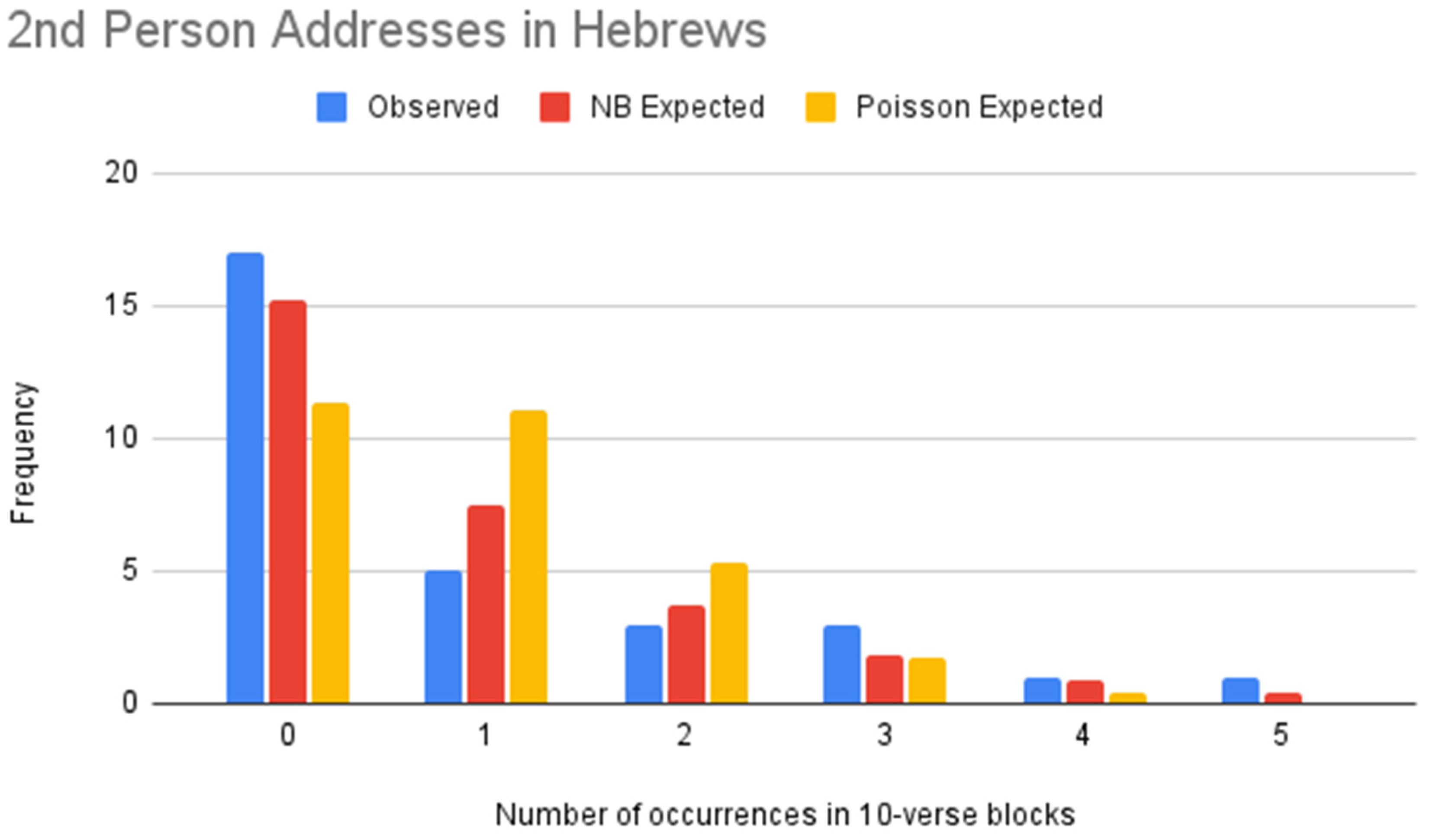
Figure 12.
NB vs. Poisson models of second person addresses (Hebrews).
Figure 12.
NB vs. Poisson models of second person addresses (Hebrews).
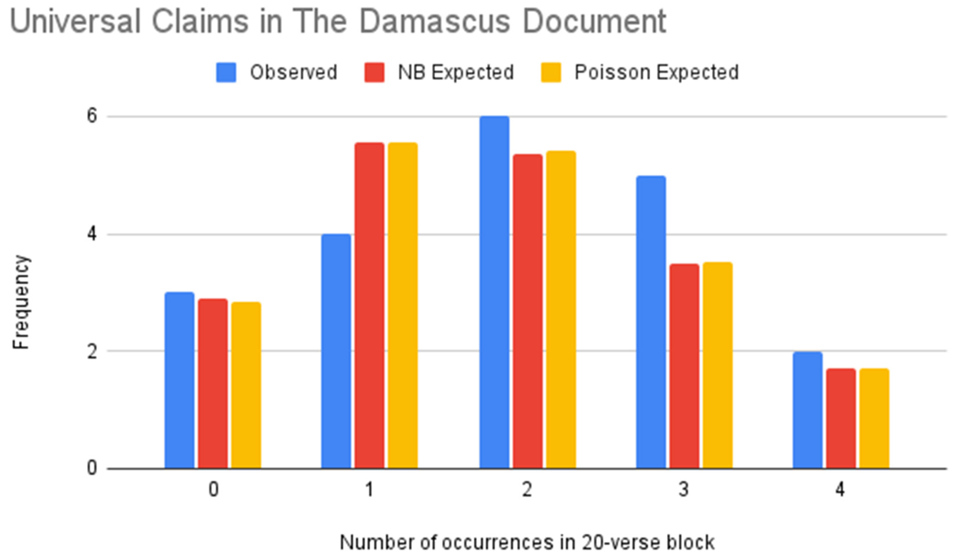
Figure 13.
NB vs. Poisson models of universal claims (Damascus Document).
Figure 13.
NB vs. Poisson models of universal claims (Damascus Document).
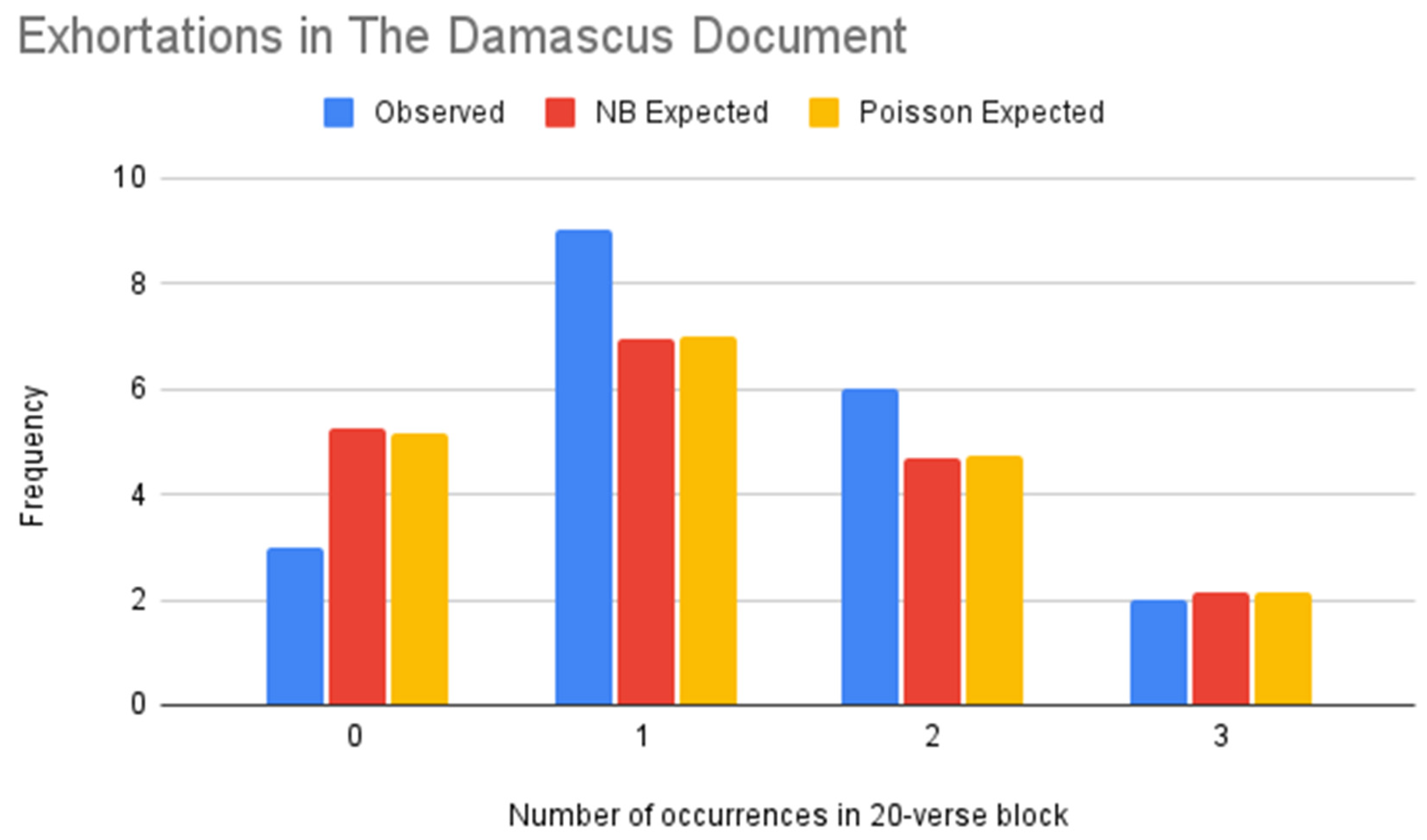
Figure 14.
NB vs. Poisson models of exhortations (Damascus Document).
Figure 14.
NB vs. Poisson models of exhortations (Damascus Document).
Figure 15.
NB vs. Poisson models of universal claims (Aristides).
Figure 15.
NB vs. Poisson models of universal claims (Aristides).
Table 1.
Summary of Goodness of Fit Tests for Paul.
Table 1.
Summary of Goodness of Fit Tests for Paul.
| | NB | Poisson |
|---|
| Exhortations | 23.80% | 12.51% |
| Imperatives | 98.78% | 31.65% |
| Universal claims | 76.83% | 70.94% |
| Second person addresses | 80.69% | 80.52% |
Table 2.
NB vs. Poisson models of exhortations (Paul).
Table 2.
NB vs. Poisson models of exhortations (Paul).
| Value | Frequency | NB Expected Frequency | Poisson Expected Frequency |
|---|
| 0 | 23 | 21.99 | 18.74 |
| 1 | 25 | 23.46 | 25.48 |
| 2 | 9 | 15.01 | 17.33 |
| 3 | 12 | 7.48 | 7.86 |
| 4 | 1 | 3.19 | 2.67 |
| 5 | 2 | 1.23 | 0.73 |
| 6 | 1 | 0.65 | 0.16 |
Table 3.
Goodness of Fit Test for exhortations (Paul).
Table 3.
Goodness of Fit Test for exhortations (Paul).
| | NB | Poisson |
|---|
| -value | 23.80% | 12.51% |
Table 4.
NB vs. Poisson models of imperatives (Paul).
Table 4.
NB vs. Poisson models of imperatives (Paul).
| Value | Frequency | NB Expected Frequency | Poisson Expected Frequency |
|---|
| 0 | 14 | 15.07 | 9.06 |
| 1 | 9 | 8.76 | 12.50 |
| 2 | 6 | 5.09 | 8.62 |
| 3 | 3 | 2.96 | 3.97 |
| 4 | 1 | 1.72 | 1.37 |
| 5 | 2 | 1.00 | 0.38 |
| 6 | 1 | 0.58 | 0.09 |
Table 5.
Goodness of Fit Test for imperatives (Paul).
Table 5.
Goodness of Fit Test for imperatives (Paul).
| | NB | Poisson |
|---|
| -value | 98.78% | 31.65% |
Table 6.
NB vs. Poisson models of universal claims (Paul).
Table 6.
NB vs. Poisson models of universal claims (Paul).
| Value | Frequency | NB Expected Frequency | Poisson Expected Frequency |
|---|
| 0 | 9 | 9.69 | 8.59 |
| 1 | 18 | 18.51 | 18.38 |
| 2 | 19 | 18.66 | 19.67 |
| 3 | 16 | 13.20 | 14.03 |
| 4 | 4 | 7.36 | 7.51 |
| 5 | 6 | 3.43 | 3.21 |
| 6 | 1 | 2.15 | 1.15 |
Table 7.
Goodness of Fit Tests for universal claims (Paul).
Table 7.
Goodness of Fit Tests for universal claims (Paul).
| | NB | Poisson |
|---|
| -value | 76.83% | 70.94% |
Table 8.
NB vs. Poisson models for second person addresses (Paul).
Table 8.
NB vs. Poisson models for second person addresses (Paul).
| Value | Frequency | NB Expected Frequency | Poisson Expected Frequency |
|---|
| 0 | 19 | 18.47 | 18.36 |
| 1 | 25 | 25.21 | 25.34 |
| 2 | 15 | 17.37 | 17.49 |
| 3 | 11 | 8.06 | 8.04 |
| 4 | 2 | 2.83 | 2.78 |
| 5 | 1 | 0.80 | 0.77 |
Table 9.
Goodness of Fit Tests for second person addresses (Paul).
Table 9.
Goodness of Fit Tests for second person addresses (Paul).
| | NB | Poisson |
|---|
| -value | 80.69% | 80.52% |
Table 10.
Summary of Goodness of Fit Tests for Epictetus.
Table 10.
Summary of Goodness of Fit Tests for Epictetus.
| | NB | Poisson |
|---|
| Exhortations | 93.04% | 41.80% |
| Imperatives | 98.64% | 27.05% |
| Universal claims | 99.33% | 17.19% |
| Second person addresses | 59.70% | 62.14% |
Table 11.
NB vs. Poisson models of exhortations (Epictetus).
Table 11.
NB vs. Poisson models of exhortations (Epictetus).
| Value | Frequency | NB Expected Frequency | Poisson Expected Frequency |
|---|
| 0 | 35 | 33.77 | 27.53 |
| 1 | 36 | 40.10 | 42.94 |
| 2 | 29 | 28.57 | 33.50 |
| 3 | 18 | 15.83 | 17.42 |
| 4 | 9 | 7.52 | 6.79 |
| 5 | 4 | 3.21 | 2.12 |
Table 12.
Goodness of Fit Tests for exhortations (Epictetus).
Table 12.
Goodness of Fit Tests for exhortations (Epictetus).
| | NB | Poisson |
|---|
| -value | 93.04% | 41.80% |
Table 13.
NB vs. Poisson models of imperatives (Epictetus).
Table 13.
NB vs. Poisson models of imperatives (Epictetus).
| Value | Frequency | NB Expected Frequency | Poisson Expected Frequency |
|---|
| 0 | 79 | 78.25 | 72.62 |
| 1 | 34 | 35.55 | 42.84 |
| 2 | 13 | 12.11 | 12.64 |
| 3 | 3 | 3.67 | 2.49 |
| 4 | 2 | 1.04 | 0.37 |
Table 14.
Goodness of Fit Tests for imperatives (Epictetus).
Table 14.
Goodness of Fit Tests for imperatives (Epictetus).
| | NB | Poisson |
|---|
| -value | 98.64% | 27.05% |
Table 15.
NB vs. Poisson models of universal claims (Epictetus).
Table 15.
NB vs. Poisson models of universal claims (Epictetus).
| Value | Frequency | NB Expected Frequency | Poisson Expected Frequency |
|---|
| 0 | 57 | 58.52 | 48.68 |
| 1 | 40 | 38.81 | 48.19 |
| 2 | 20 | 19.31 | 23.85 |
| 3 | 9 | 8.54 | 7.87 |
| 4 | 2 | 3.54 | 1.95 |
| 5 | 3 | 1.41 | 0.39 |
Table 16.
Goodness of Fit Tests for universal claims (Epictetus).
Table 16.
Goodness of Fit Tests for universal claims (Epictetus).
| | NB | Poisson |
|---|
| -value | 99.33% | 17.19% |
Table 17.
NB vs. Poisson models of second person addresses (Epictetus).
Table 17.
NB vs. Poisson models of second person addresses (Epictetus).
| Value | Frequency | NB Expected Frequency | Poisson Expected Frequency |
|---|
| 0 | 56 | 59.86 | 60.05 |
| 1 | 54 | 46.70 | 46.84 |
| 2 | 16 | 18.40 | 18.27 |
| 3 | 3 | 4.88 | 4.75 |
| 4 | 2 | 0.98 | 0.93 |
Table 18.
Goodness of Fit Tests for second person addresses (Epictetus).
Table 18.
Goodness of Fit Tests for second person addresses (Epictetus).
| | NB | Poisson |
|---|
| -value | 59.70% | 62.14% |
Table 19.
NB vs. Poisson models of universal claims (4 Maccabees).
Table 19.
NB vs. Poisson models of universal claims (4 Maccabees).
| Value | Frequency | NB Expected Frequency | Poisson Expected Frequency |
|---|
| 0 | 8 | 8.55 | 7.35 |
| 1 | 6 | 6.64 | 7.72 |
| 2 | 5 | 3.44 | 4.05 |
| 3 | 2 | 1.48 | 1.42 |
Table 20.
Goodness of Fit Tests for universal claims (4 Maccabees).
Table 20.
Goodness of Fit Tests for universal claims (4 Maccabees).
| | NB | Poisson |
|---|
| -value | 84.35% | 63.04% |
Table 21.
Summary of Goodness of Fit Tests for Hebrews.
Table 21.
Summary of Goodness of Fit Tests for Hebrews.
| | NB | Poisson |
|---|
| Exhortations | 96.89% | 65.36% |
| Universal claims | 43.88% | 43.64% |
| Second person addresses | 62.82% | 1.48% |
Table 22.
NB vs. Poisson models of second person addresses (Hebrews).
Table 22.
NB vs. Poisson models of second person addresses (Hebrews).
| Value | Frequency | NB Expected Frequency | Poisson Expected Frequency |
|---|
| 0 | 15 | 14.60 | 12.57 |
| 1 | 9 | 8.83 | 10.93 |
| 2 | 3 | 4.00 | 4.76 |
| 3 | 1 | 1.61 | 1.38 |
| 4 | 2 | 0.61 | 0.30 |
Table 23.
Goodness of Fit Tests for exhortation (Hebrews).
Table 23.
Goodness of Fit Tests for exhortation (Hebrews).
| | NB | Poisson |
|---|
| -value | 96.89% | 65.36% |
Table 24.
NB vs. Poisson models of universal claims (Hebrews).
Table 24.
NB vs. Poisson models of universal claims (Hebrews).
| Value | Frequency | NB Expected Frequency | Poisson Expected Frequency |
|---|
| 0 | 5 | 4.57 | 4.49 |
| 1 | 9 | 8.52 | 8.52 |
| 2 | 4 | 8.02 | 8.10 |
| 3 | 8 | 5.08 | 5.13 |
| 4 | 4 | 2.44 | 2.44 |
Table 25.
Goodness of Fit Tests for universal claims (Hebrews).
Table 25.
Goodness of Fit Tests for universal claims (Hebrews).
| | NB | Poisson |
|---|
| -value | 43.88% | 43.64% |
Table 26.
NB vs. Poisson models of second person addresses (Hebrews).
Table 26.
NB vs. Poisson models of second person addresses (Hebrews).
| Value | Frequency | NB Expected Frequency | Poisson Expected Frequency |
|---|
| 0 | 17 | 15.25 | 11.37 |
| 1 | 5 | 7.50 | 11.03 |
| 2 | 3 | 3.69 | 5.35 |
| 3 | 3 | 1.81 | 1.73 |
| 4 | 1 | 0.89 | 0.42 |
| 5 | 1 | 0.44 | 0.08 |
Table 27.
Goodness of Fit Tests for second person addresses (Hebrews).
Table 27.
Goodness of Fit Tests for second person addresses (Hebrews).
| | NB | Poisson |
|---|
| -value | 62.82% | 1.48% |
Table 28.
NB vs. Poisson models of universal claims (Damascus Document).
Table 28.
NB vs. Poisson models of universal claims (Damascus Document).
| Value | Frequency | NB Expected Frequency | Poisson Expected Frequency |
|---|
| 0 | 3 | 2.90 | 2.85 |
| 1 | 4 | 5.55 | 5.55 |
| 2 | 6 | 5.36 | 5.41 |
| 3 | 5 | 3.48 | 3.52 |
| 4 | 2 | 1.72 | 1.71 |
Table 29.
Goodness of Fit Tests for universal claims (Damascus Document).
Table 29.
Goodness of Fit Tests for universal claims (Damascus Document).
| | NB | Poisson |
|---|
| -value | 89.29% | 89.43% |
Table 30.
NB vs. Poisson models of exhortations (Damascus Document).
Table 30.
NB vs. Poisson models of exhortations (Damascus Document).
| Value | Frequency | NB Expected Frequency | Poisson Expected Frequency |
|---|
| 0 | 3 | 5.23 | 5.18 |
| 1 | 9 | 6.97 | 7.00 |
| 2 | 6 | 4.69 | 4.72 |
| 3 | 2 | 2.12 | 2.13 |
Table 31.
Goodness of Fit Tests for exhortations (Damascus Document).
Table 31.
Goodness of Fit Tests for exhortations (Damascus Document).
| | NB | Poisson |
|---|
| -value | 46.09% | 47.31% |
Table 32.
NB vs. Poisson models of universal claims (Aristides).
Table 32.
NB vs. Poisson models of universal claims (Aristides).
| Value | Frequency | NB Expected Frequency | Poisson Expected Frequency |
|---|
| 0 | 0 | 3.59 | 3.52 |
| 1 | 5 | 6.76 | 6.76 |
| 2 | 16 | 6.42 | 6.48 |
| 3 | 3 | 4.11 | 4.15 |
Table 33.
Goodness of Fit Tests for universal claims (Aristides).
Table 33.
Goodness of Fit Tests for universal claims (Aristides).
| | NB | Poisson |
|---|
| -value | 0.01% | 0.01% |
Table 34.
Summary of NB vs. Poisson models of exhortations.
Table 34.
Summary of NB vs. Poisson models of exhortations.
| Exhortations | | |
|---|
| | NB | Poisson |
| Paul | 23.80% | 12.51% |
| Epictetus | 93.04% | 41.80% |
| Hebrews | 96.89% | 65.36% |
| Damascus Document | 46.09% | 47.31% |
Table 35.
Summary of NB vs. Poisson models of imperatives.
Table 35.
Summary of NB vs. Poisson models of imperatives.
| Imperatives | | |
|---|
| | NB | Poisson |
| Paul | 98.78% | 31.65% |
| Epictetus | 98.64% | 27.05% |
Table 36.
Summary of NB vs. Poisson models of universal claims.
Table 36.
Summary of NB vs. Poisson models of universal claims.
| Universal Claims | | |
|---|
| | NB | Poisson |
| Paul | 76.83% | 70.94% |
| Epictetus | 99.33% | 17.19% |
| Hebrews | 43.88% | 43.64% |
| 4 Maccabees | 84.35% | 63.04% |
| Damascus Document | 89.29% | 89.43% |
| Aristides | 0.01% | 0.01% |
Table 37.
Summary of NB vs. Poisson models of second person addresses.
Table 37.
Summary of NB vs. Poisson models of second person addresses.
| Second Person Addresses | | |
|---|
| | NB | Poisson |
| Paul | 80.69% | 80.52% |
| Epictetus | 59.70% | 62.14% |
| Hebrews | 62.82% | 1.48% |
Table 38.
NB vs. Poisson models for full text of 1 Cor.
Table 38.
NB vs. Poisson models for full text of 1 Cor.
| Value | Frequency | NB Expected Frequency | Poisson Expected Frequency |
|---|
| 0 | 20 | 20.64 | 19.52 |
| 1 | 15 | 14.09 | 15.42 |
| 2 | 5 | 5.77 | 6.09 |
| 3 | 3 | 1.84 | 1.60 |
Table 39.
Goodness of Fit Tests for full text of 1 Cor.
Table 39.
Goodness of Fit Tests for full text of 1 Cor.
| | NB | Poisson |
|---|
| -value | 96.35% | 86.22% |
Table 40.
NB vs. Poisson models for 1 Cor with verses removed.
Table 40.
NB vs. Poisson models for 1 Cor with verses removed.
| Value | Frequency | NB Expected Frequency | Poisson Expected Frequency |
|---|
| 0 | 19 | 20.51 | 18.68 |
| 1 | 16 | 13.08 | 15.13 |
| 2 | 3 | 5.56 | 6.13 |
| 3 | 4 | 1.97 | 1.65 |
Table 41.
Goodness of Fit Tests for 1 Cor with verses removed.
Table 41.
Goodness of Fit Tests for 1 Cor with verses removed.
| | NB | Poisson |
|---|
| -value | 49.34% | 32.07% |
Table 42.
NB vs. Poisson models for full text of 2 Cor.
Table 42.
NB vs. Poisson models for full text of 2 Cor.
| Value | Frequency | NB Expected Frequency | Poisson Expected Frequency |
|---|
| 0 | 14 | 13.51 | 13.18 |
| 1 | 8 | 8.00 | 8.44 |
| 2 | 1 | 2.67 | 2.70 |
| 3 | 2 | 0.66 | 0.58 |
Table 43.
Goodness of Fit Tests for full text of 2 Cor.
Table 43.
Goodness of Fit Tests for full text of 2 Cor.
| | NB | Poisson |
|---|
| -value | 95.76% | 94.35% |
Table 44.
NB vs. Poisson models for 2 Cor with verses removed.
Table 44.
NB vs. Poisson models for 2 Cor with verses removed.
| Value | Frequency | NB Expected Frequency | Poisson Expected Frequency |
|---|
| 0 | 15 | 15.63 | 13.72 |
| 1 | 6 | 5.86 | 8.23 |
| 2 | 3 | 2.20 | 2.47 |
| 3 | 1 | 0.82 | 0.49 |
Table 45.
Goodness of Fit Tests for 2 Cor with verses removed.
Table 45.
Goodness of Fit Tests for 2 Cor with verses removed.
| | NB | Poisson |
|---|
| -value | 95.36% | 59.98% |
Table 46.
Control statistics for 1 Cor.
Table 46.
Control statistics for 1 Cor.
| 1 Corinthians | | |
|---|
| Passage removed | VMR | Skewness |
| 1:15–1:31 | 0.8580 | 0.6443 |
| 4:11–5:06 | 0.9024 | 0.6907 |
| 6:9–7:5 | 0.9024 | 0.6907 |
| 7:33–8:9 | 0.9645 | 0.9079 |
| 8:11–9:14 | 0.9645 | 0.9079 |
| 10:4–10:20 | 0.9953 | 1.0339 |
| 10:18–11:1 | 0.9756 | 1.1212 |
| 12:7–12:23 | 1.0387 | 0.9961 |
| 13:4–14:7 | 1.1402 | 1.0756 |
| 13:10–14:13 | 1.1275 | 1.1660 |
| | Mean | Median | Standard Deviation |
| VMR | 0.9869 | 0.9701 | 0.0931 |
| Skew | 0.9234 | 0.9520 | 0.1901 |
Table 47.
Control statistics for 2 Cor.
Table 47.
Control statistics for 2 Cor.
| 2 Corinthians | | |
|---|
| Passage removed | VMR | Skewness |
| 2:11–2:16 | 0.9461 | 0.6707 |
| 4:4–4:9 | 0.9461 | 0.6707 |
| 4:6–4:11 | 0.9461 | 0.6707 |
| 5:1–5:6 | 1.0260 | 0.7819 |
| 5:4–5:9 | 1.0260 | 0.7819 |
| 9:7–9:12 | 1.2865 | 1.5463 |
| 10:13–10:18 | 1.3137 | 1.3625 |
| 10:14–11:1 | 1.3137 | 1.3625 |
| 11:19–11:24 | 1.2865 | 1.5432 |
| 12:14–12:19 | 1.3137 | 1.3625 |
| | Mean | Median | Standard Deviation |
| VMR | 1.1404 | 1.1563 | 0.1739 |
| Skewness | 1.0756 | 1.0722 | 0.3879 |
Table 48.
Results for 1 Cor.
Table 48.
Results for 1 Cor.
| 1 Corinthians | | |
|---|
| | Full Text | Verses removed |
| -value Poisson | 86.22% | 32.07% |
| -value NB | 96.35% | 49.34% |
| VMR | 1.0574 | 1.0990 |
| Skewness | 1.0270 | 1.1333 |
Table 49.
Results for 2 Cor.
Table 49.
Results for 2 Cor.
| 2 Corinthians | | |
|---|
| | Full text | Verses removed |
| -value Poisson | 94.35% | 59.98% |
| -value NB | 95.76% | 95.36% |
| VMR | 1.2865 | 1.25 |
| Skewness | 1.5463 | 1.3388 |


