
Mean Current Profile over Rippled-Beds in the Presence of Non-Breaking Waves and Analysis of Its Influencing Factors

Abstract
:1. Introduction
2. Materials and Methods
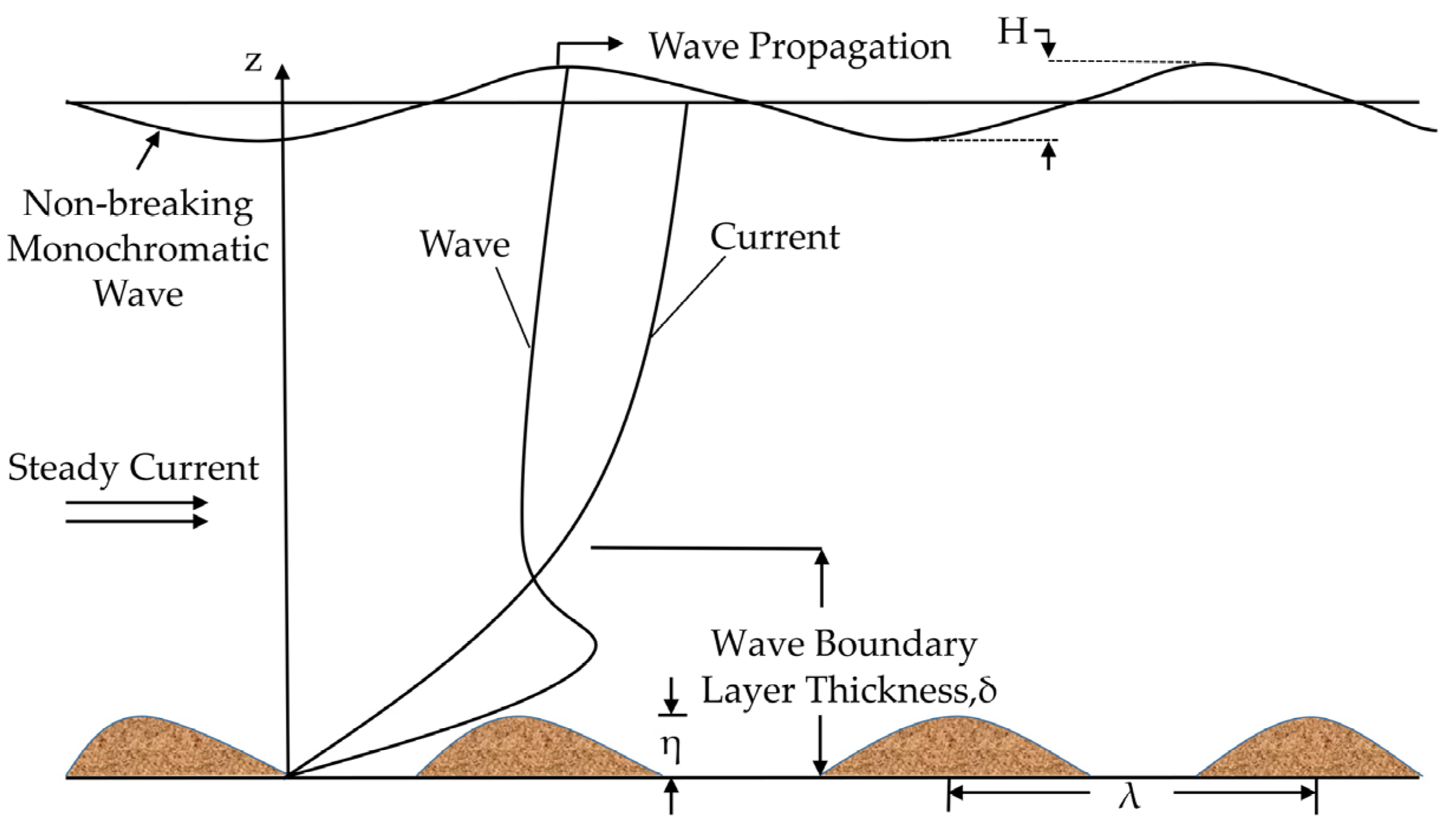
2.1. Governing Equations
2.2. Bed Form and the Bed Roughness
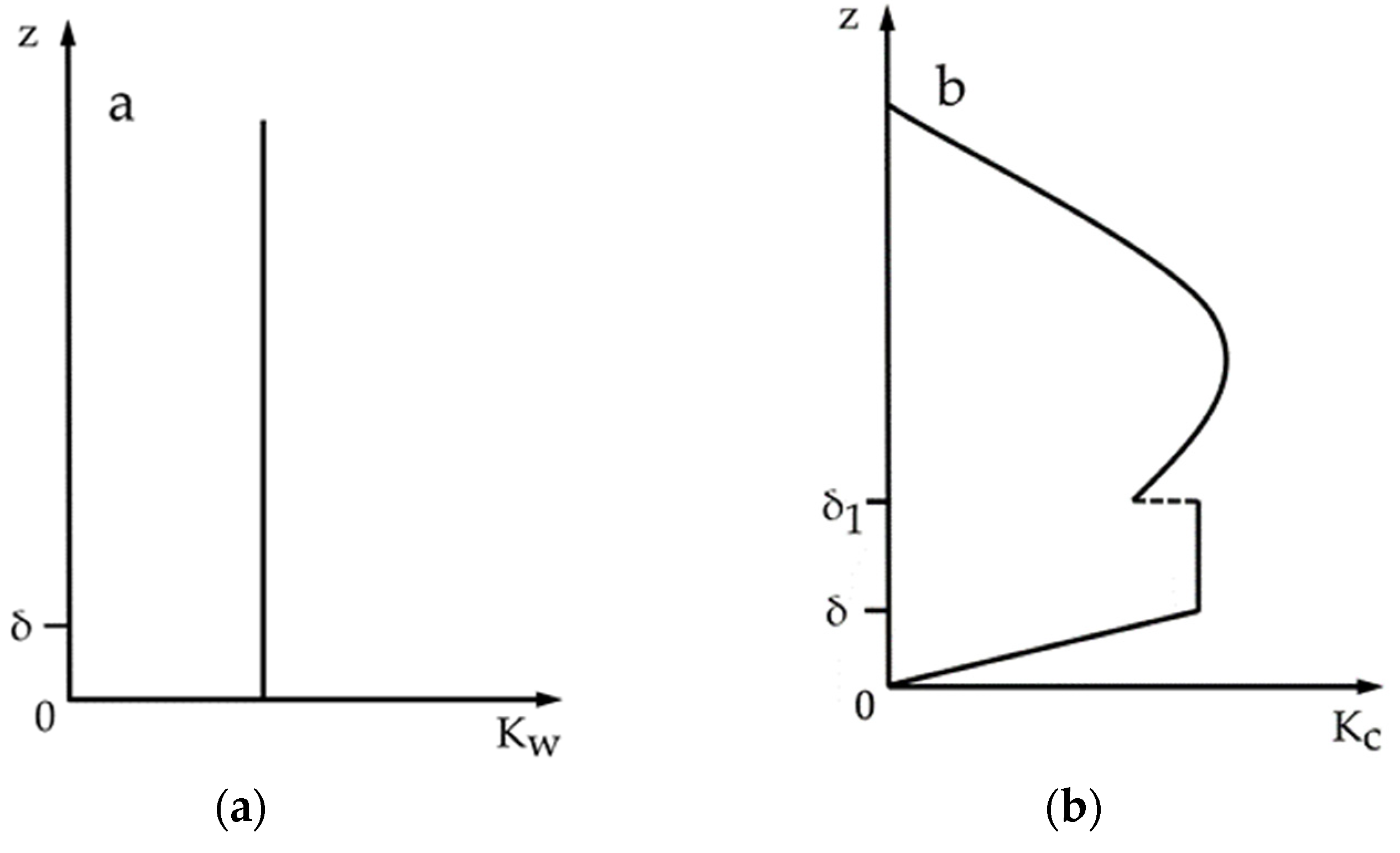
2.3. Eddy Viscosities
2.4. Solutions of and
2.4.1. Solution of
2.4.2. Solution of
2.5. Shear Velocities and Wave Friction Factor
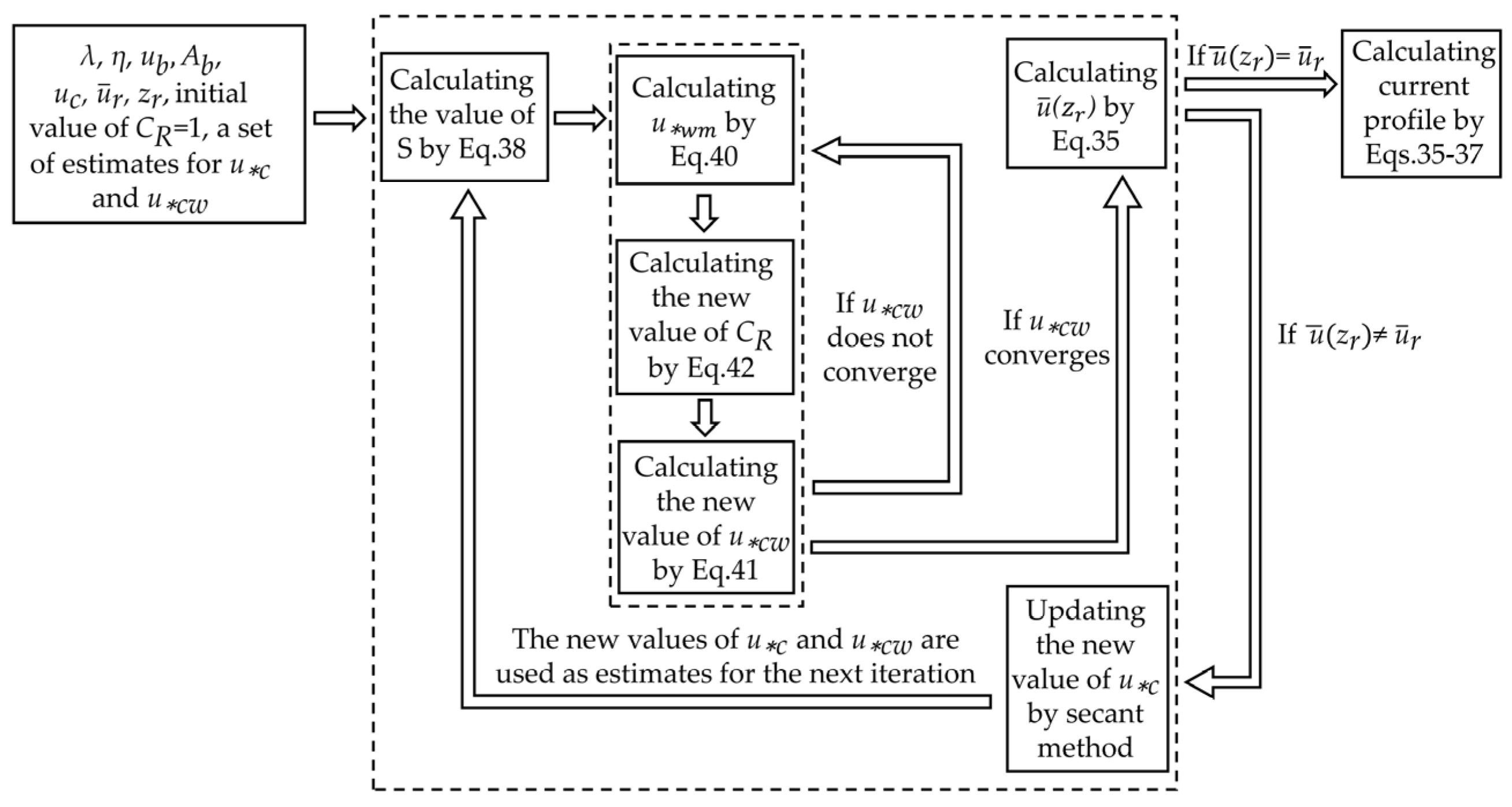
2.6. Solution Procedure
- The initial was equal to 1. The value of can be calculated by Equation (40), then a new value of can be obtained by substituting and into Equation (42). The value of can be derived by substituting and into Equation (41).
- Repeat step (1) until converges. This is the inner loop.
- Calculate the mean current profile using Equations (35)–(37). If the calculated value of , then the process from step (1) is repeated with a new until the calculated is equal to . This is the outer loop.
3. Predictions of Boundary Layer Thickness and Bed Roughness
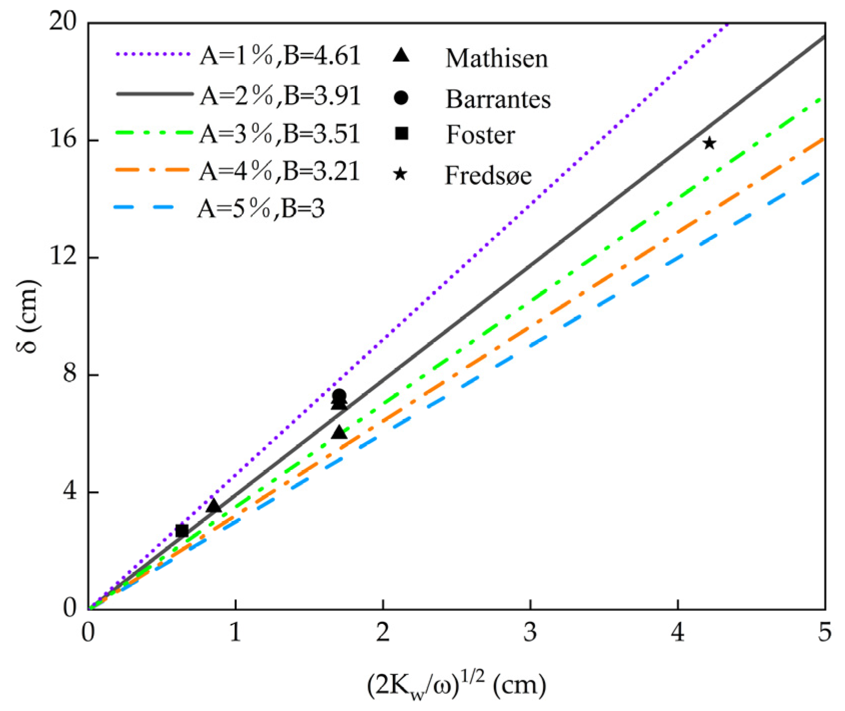
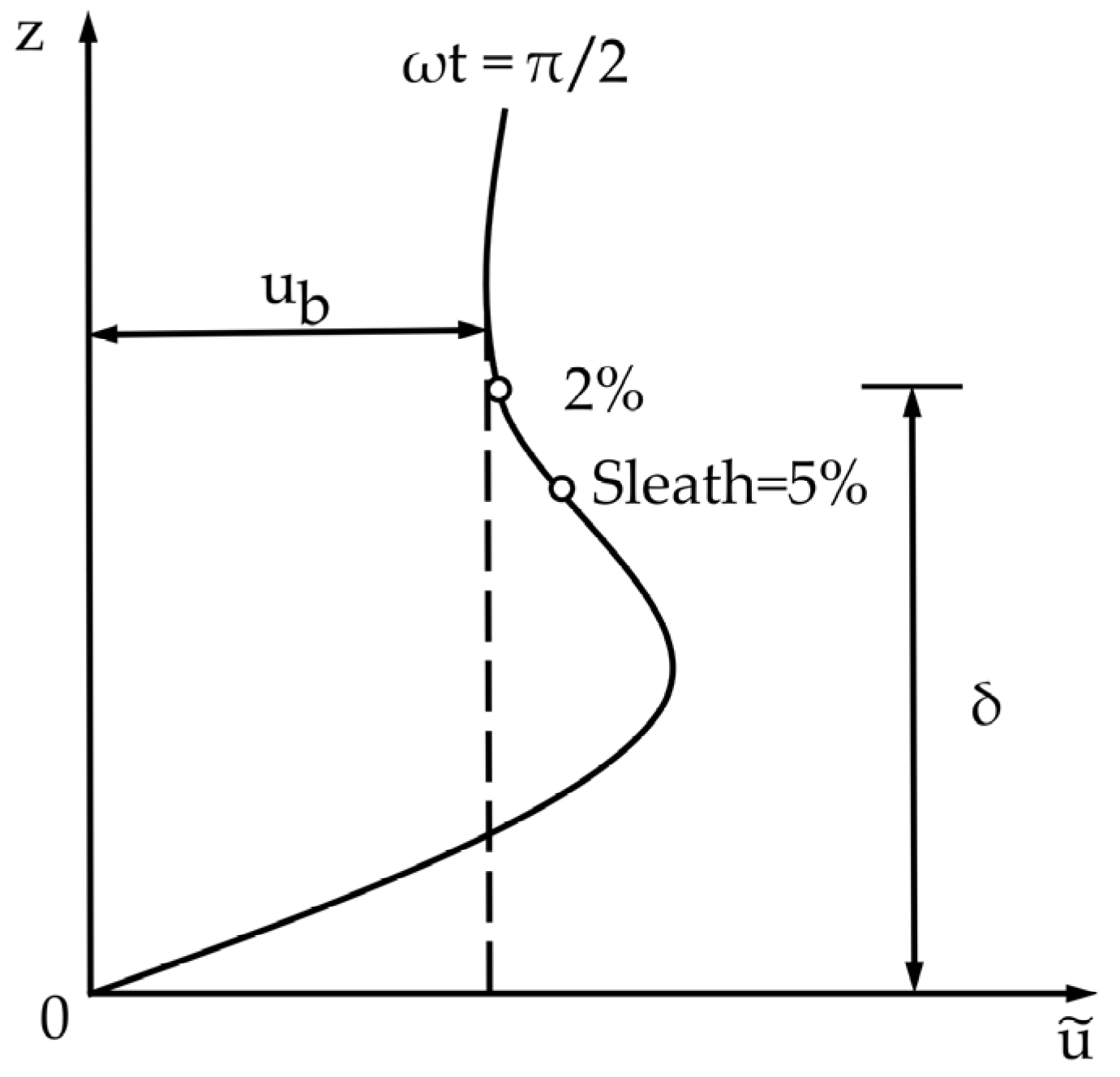
3.1. Thickness of the Wave Boundary Layer
3.2. Physical Bed Roughness and Apparent Bed Roughness
- There is a distinct trend where increase with , where is the depth-averaged current velocity. When is positive, . These conclusions are similar to those summarized in [10].
- For a given , increase with H/h, that is, the higher the waves, the larger the apparent bed roughness.
- For a given , is supposed to be a potential impact factor for . Unfortunately, no exact effect of on can be identified. In addition, when , will be smaller with increasing . This may be because has little effect on .
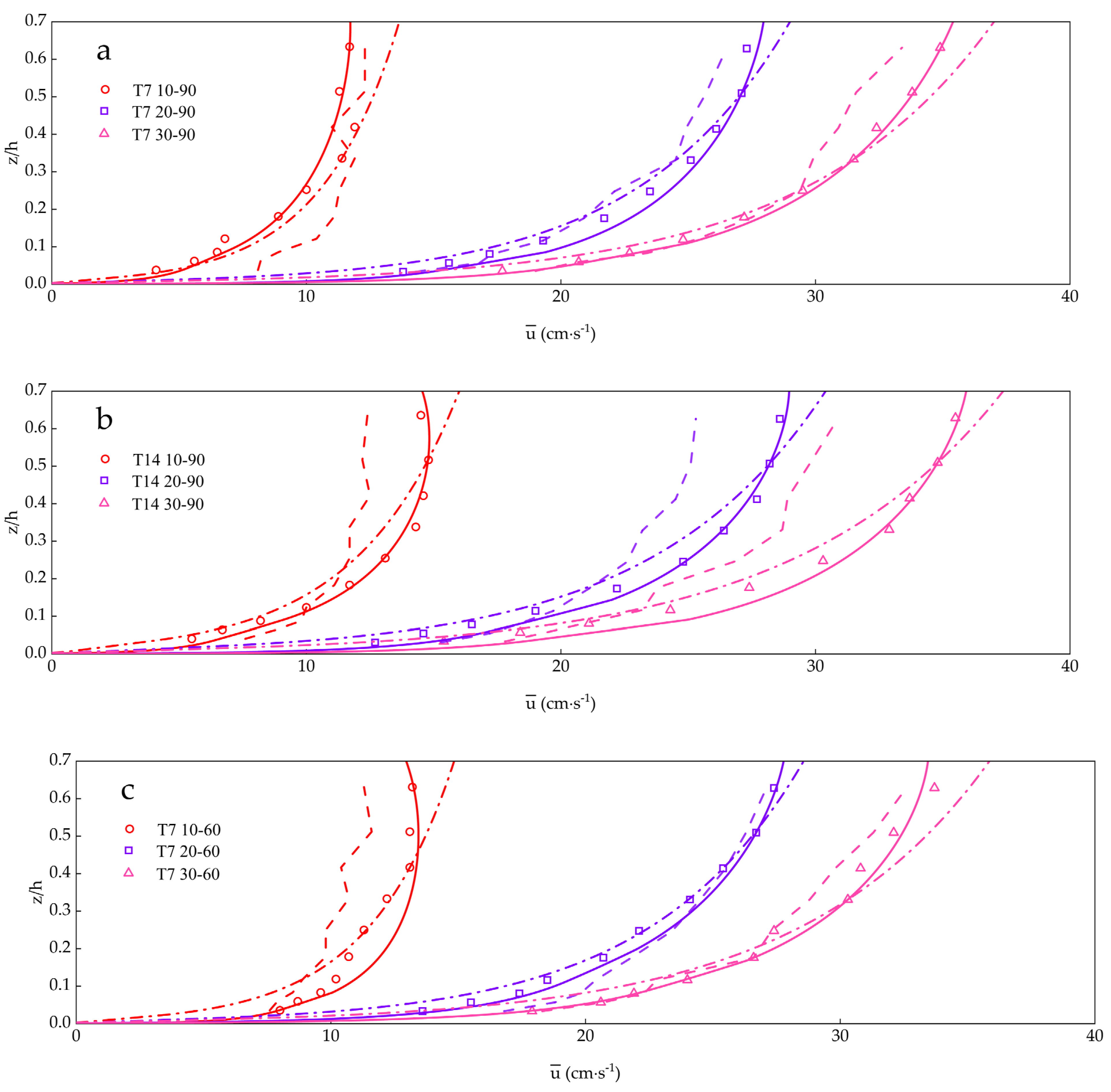
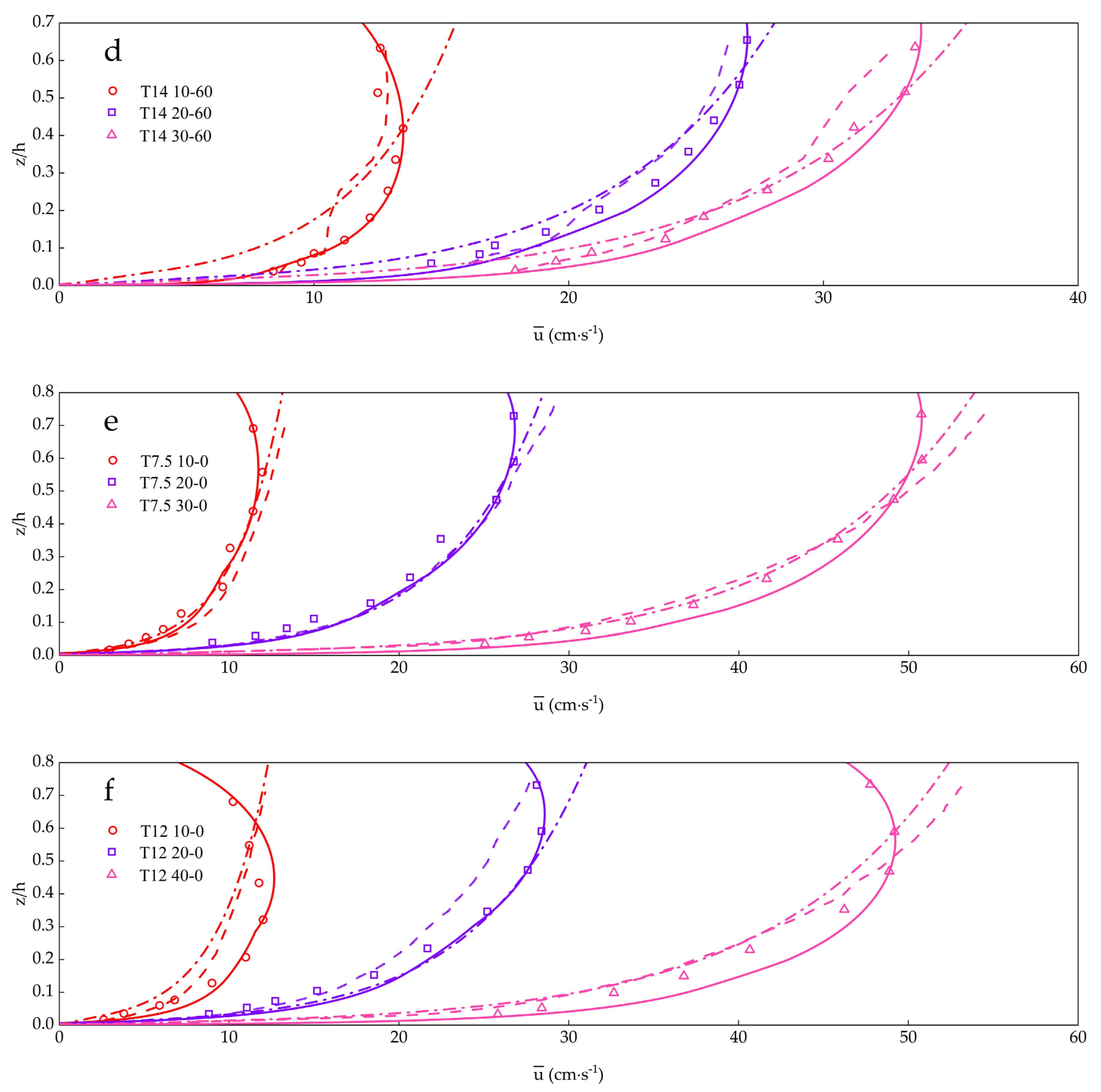
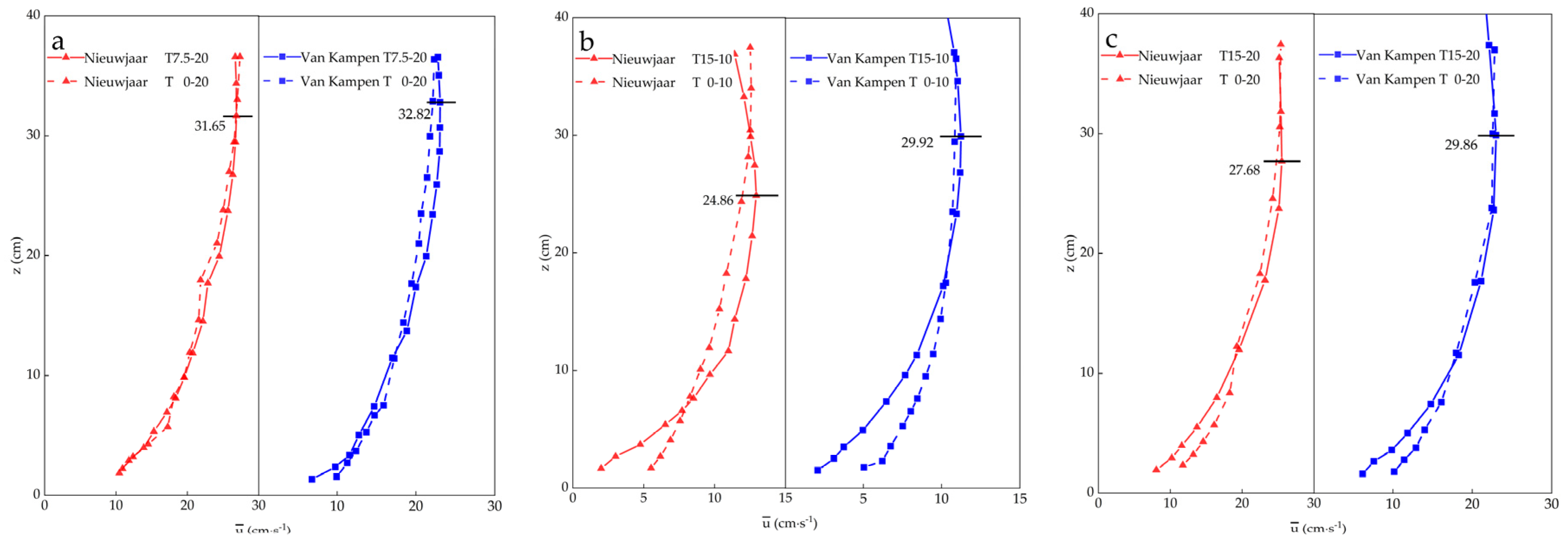
4. Results
5. Discussion
- In the near-bed layer (z/h < 0.2) and near-surface layer (z/h > 0.6), the presence of waves leads to a reduction in the current velocities, and an enhancement in the middle layer.
- The deviation of the current velocity profile caused by the presence of waves is relatively notable when the free stream wave orbital velocity, , is relatively large with respect to the depth-averaged current velocity .
- For a given and , the smaller the , the lower is the level at which the current velocities begin to decrease.
6. Conclusions
Author Contributions
Funding
Institutional Review Board Statement
Informed Consent Statement
Data Availability Statement
Acknowledgments
Conflicts of Interest
References
- Pao, C.H.; Chen, J.L.; Su, S.F.; Huang, Y.-C.; Huang, W.-H.; Kuo, C.-H. The Effect of Wave-Induced Current and Coastal Structure on Sediment Transport at the Zengwen River Mouth. J. Mar. Sci. Eng. 2021, 9, 333. [Google Scholar] [CrossRef]
- Mahmoodi, A.; Lashteh Neshaei, M.A.; Mansouri, A.; Bejestan, M.S. Study of current-and wave-induced sediment transport in the Nowshahr Port entrance channel by using numerical modeling and field measurements. J. Mar. Sci. Eng. 2020, 8, 284. [Google Scholar] [CrossRef] [Green Version]
- Peng, Y.; Yu, Q.; Wang, Y.; Zhu, Q.; Wang, Y.P. Sensitivities of Bottom Stress Estimation to Sediment Stratification in a Tidal Coastal Bottom Boundary Layer. J. Mar. Sci. Eng. 2020, 8, 256. [Google Scholar] [CrossRef] [Green Version]
- Kuang, C.; Han, X.; Zhang, J.; Zou, Q.; Dong, B. Morphodynamic Evolution of a Nourished Beach with Artificial Sandbars: Field Observations and Numerical Modeling. J. Mar. Sci. Eng. 2021, 9, 245. [Google Scholar] [CrossRef]
- Ruggeri, A.; Musumeci, R.E.; Faraci, C. Wave-Current Flow and Vorticity Close to a Fixed Rippled Bed. J. Mar. Sci. Eng. 2020, 8, 867. [Google Scholar] [CrossRef]
- Birrien, F.; Baldock, T. A Coupled Hydrodynamic-Equilibrium Type Beach Profile Evolution Model. J. Mar. Sci. Eng. 2021, 9, 353. [Google Scholar] [CrossRef]
- Li, M.Z.; Amos, C.L. Sheet flow and large wave ripples under combined waves and currents: Field observations, model predictions and effects on boundary layer dynamics. Cont. Shelf Res. 1999, 19, 637–663. [Google Scholar] [CrossRef]
- Nielsen, P. Coastal Bottom Boundary Layers and Sediment Transport; World Scientific: Singapore, 1992. [Google Scholar]
- Van Rijn, L.C. Principles of Fluid Flow and Surface Waves in Rivers, Estuaries, Seas and Oceans; Aqua Publications: Amsterdam, The Netherlands, 1990. [Google Scholar]
- Fredsøe, J.; Andersen, K.H.; Sumer, B.M. Wave plus current over a ripple-covered bed. Coast. Eng. 1999, 38, 177–221. [Google Scholar] [CrossRef]
- Bakker, W.T.; Van Doorn, T. Near-bottom velocities in waves with a current. Coast. Eng. 1978, 1978, 1394–1413. [Google Scholar] [CrossRef]
- Kemp, P.H.; Simons, R.R. The interaction between waves and a turbulent current: Waves propagating with the current. J. Fluid Mech. 1982, 116, 227–250. [Google Scholar] [CrossRef] [Green Version]
- Mathisen, P.P.; Madsen, O.S. Waves and currents over a fixed rippled bed: 2. Bottom and apparent roughness experienced by currents in the presence of waves. J. Geophys. Res. Ocean. 1996, 101, 16543–16550. [Google Scholar] [CrossRef]
- Grant, W.D.; Madsen, O.S. Combined wave and current interaction with a rough bottom. J. Geophys. Res. Ocean. 1979, 84, 1797–1808. [Google Scholar] [CrossRef]
- Christoffersen, J.B.; Jonsson, I.G. Bed friction and dissipation in a combined current and wave motion. Ocean Eng. 1985, 12, 387–423. [Google Scholar] [CrossRef]
- Styles, R.; Glenn, S.M. Modeling stratified wave and current bottom boundary layers on the continental shelf. J. Geophys. Res. 2000, 105, 24119–24139. [Google Scholar] [CrossRef] [Green Version]
- Styles, R.; Glenn, S.M.; Brown, M.E. An Optimized Combined Wave and Current Bottom Boundary Layer Model for Arbitrary Bed Roughness; Coastal and Hydraulics Laboratory, US Army Engineer Research and Development Center: Vicksburg, MS, USA, 2017; Available online: https://www.semanticscholar.org/paper/An-Optimized-Combined-Wave-and-Current-Bottom-Layer-Styles-Glenn/48048be333db48df8f857d97162b8251b442e2af (accessed on 7 September 2021).
- You, Z.J. Eddy viscosities and velocities in combined wave-current flows. Ocean Eng. 1994, 21, 81–97. [Google Scholar] [CrossRef]
- Trowbridge, J.; Madsen, O.S. Turbulent wave boundary layers: 2. Second-order theory and mass transport. J. Geophys. Res. 1984, 89, 7999–8007. [Google Scholar] [CrossRef]
- Foster, D.L.; Guenther, R.A.; Holman, R.A. An analytic solution to the wave bottom boundary layer governing equation under arbitrary wave forcing. Ocean Eng. 1999, 26, 595–623. [Google Scholar] [CrossRef]
- Styles, R.; Bryant, D.B. Combined Wave and Current Bottom Boundary Layers: A Review; ERDC-CHL-SR-16-1; Army Engineer Research and Development Center: Vicksburg, MS, USA, 2016. [Google Scholar]
- Davies, A.G.; Soulsby, R.L.; King, H.L. A numerical model of the combined wave and current bottom boundary layer. J. Geophys. Res. Ocean. 1988, 93, 491–508. [Google Scholar] [CrossRef]
- Soulsby, R.L.; Hamm, L.; Klopman, G.; Myrhaug, D.; Simons, R.; Thomas, G. Wave-current interaction within and outside the bottom boundary layer. Coast. Eng. 1993, 21, 41–69. [Google Scholar] [CrossRef]
- Shi, J.Z.; Wang, Y. The vertical structure of combined wave–current flow. Ocean Eng. 2008, 35, 174–181. [Google Scholar] [CrossRef]
- Faraci, C.; Foti, E.; Musumeci, R.E. Waves plus currents at a right angle: The rippled bed case. J. Geophys. Res. Ocean. 2008, 113, C07018. [Google Scholar] [CrossRef] [Green Version]
- Smaoui, H.; Kaidi, S. Bed Shear Stresses Parameterization in Wave–Current Interaction by k−ω Turbulence Model. Int. J. Appl. Mech. 2017, 9, 1750059. [Google Scholar] [CrossRef]
- Zuo, L. Modelling and Analysis of Fine Sediment Transport in Wave-Current Bottom Boundary Layer; CRC Press: Boca Raton, FL, USA, 2018. [Google Scholar]
- You, Z.J.; Wilkinson, D.L.; Nielsen, P. Velocity distributions of waves and currents in the combined flow. Coast. Eng. 1991, 15, 525–543. [Google Scholar] [CrossRef]
- You, Z.J. The effect of wave-induced stress on current profiles. Ocean Eng. 1996, 23, 619–628. [Google Scholar] [CrossRef]
- Sutherland, J.; Battjes, J.A. Wave Reynolds Stress and Its Effect on the Undertow Model. Master’s Thesis, Technical University of Delft, Delft, The Netherlands, 1995. [Google Scholar]
- Peter, N.; You, Z.J. Eulerian mean velocities under non-breaking waves on horizontal bottoms. Proc. Coast. Eng. Conf. 1997, 4, 4066–4077. [Google Scholar] [CrossRef]
- Longuet-Higgins, M.S. The mechanics of the boundary layer near the bottom in a progressive wave. In Proceedings of the 6th International Conference on Coastal Engineering; ASCE: Berkeley, CA, USA, 1958; Volume 184, p. 193. [Google Scholar]
- Supharatid, S.; Tanaka, H.; Shuto, N. Interactions of waves and current (Part I: Experimental investigation). Coast. Eng. Jpn. 1992, 35, 167–186. [Google Scholar] [CrossRef]
- Chun, H.; Suh, K.D. Wave-induced Reynolds stress in three-dimensional nearshore currents model. J. Coast. Res. 2016, 32, 898–910. [Google Scholar] [CrossRef]
- Davies, A.G.; Villaret, C. Eulerian drift induced by progressive waves above rippled and very rough beds. J. Geophys. Res. Ocean. 1999, 104, 1465–1488. [Google Scholar] [CrossRef] [Green Version]
- Van der, A.D.A. 1DV Modelling of Wave-Induced Sand Transport Processes over Rippled Beds. Master’s Thesis, University of Twente, Enschede, The Netherlands, 2005. [Google Scholar]
- Nielsen, P. 1DV structure of turbulent wave boundary layers. Coast. Eng. 2016, 112, 1–8. [Google Scholar] [CrossRef]
- Grant, W.D.; Madsen, O.S. Movable bed roughness in unsteady oscillatory flow. J. Geophys. Res. Ocean. 1982, 87, 469–481. [Google Scholar] [CrossRef]
- Salles, P.A.A. Eddy Viscosity Models for Pure Waves over Large Roughness Elements. Master’s Thesis, Massachusetts Institute of Technology, Cambridge, MA, USA, 1997. [Google Scholar]
- Sleath, J.F.A. Turbulent oscillatory flow over rough beds. J. Fluid Mech. 1987, 182, 369–409. [Google Scholar] [CrossRef]
- Mathisen, P.P. Bottom Roughness for Wave and Current Boundary Layer Flows over a Rippled Bed. Ph.D. Thesis, Massachusetts Institute of Technology, Cambridge, MA, USA, 1993. [Google Scholar]
- Barrantes, A.I. Turbulent boundary layer flow over two-dimensional bottom roughness elements. Ph.D. Thesis, Massachusetts Institute of Technology, Cambridge, MA, USA, 1997. [Google Scholar]
- Rodríguez-Abudo, S.; Foster, D.L. Direct estimates of friction factors for a mobile rippled bed. J. Geophys. Res. Ocean. 2017, 122, 80–92. [Google Scholar] [CrossRef]
- Van der Kaaij, T.H.; Nieuwjaar, M.W.C. Sediment Concentrations and Transport in Case of Irregular Non-Breaking Waves with a Current, Part A and B. Master’s Thesis, Delft University of Technology, Delft, The Netherlands, 1987. Available online: https://repository.tudelft.nl/islandora/object/uuid%3Ac4267aec-cca1-4de8-bdb7-77e40a236829 (accessed on 7 September 2021).
- Nap, E.; Van Kampen, A. Sediment Concentrations and Transport in Case of Irregular Non-Breaking Waves with a Current, Part A and B. Master’s Thesis, Delft University of Technology, Delft, The Netherlands, 1988. Available online: https://repository.tudelft.nl/islandora/object/uuid%3Ad079b281-a758-440d-badc-4e41a848bca5 (accessed on 7 September 2021).
- Havinga, F.J. Sediment Concentrations and Sediment Transport in Case of Irregular Non-Breaking Waves with a Current. Master’s Thesis, Delft University of Technology, Delft, The Netherlands, 1992. Available online: https://repository.tudelft.nl/islandora/object/uuid:b57004ae-f32c-4083-8789-58788a55626a (accessed on 7 September 2021).
- Mathisen, P.P.; Madsen, O.S. Waves and currents over a fixed rippled bed: 1. Bottom roughness experienced by waves in the presence and absence of currents. J. Geophys. Res. Ocean. 1996, 101, 16533–16542. [Google Scholar] [CrossRef]
- Van Rijn, L.C. Unified view of sediment transport by currents and waves. I: Initiation of motion, bed roughness, and bed-load transport. J. Hydraul. Eng. 2007, 133, 649–667. [Google Scholar] [CrossRef] [Green Version]
- Sleath, J.F.A. Velocities and shear stresses in wave-current flows. J. Geophys. Res. Ocean. 1991, 96, 15237–15244. [Google Scholar] [CrossRef]
- Willmott, C.J.; Feddema, J.J.; Klink, K.; LeGates, D.R.; O’Donnell, J.; Rowe, C.M. Statistics for the evaluation and comparison of models. J. Geophys. Res. Ocean. 1985, 90, 8995–9005. [Google Scholar] [CrossRef] [Green Version]
- Madsen, O.S.; Salles, P. Eddy viscosity models for wave boundary layers. Coast. Eng. 1998, 26, 2615–2627. [Google Scholar] [CrossRef]
- Bijker, E.W.; Kalkwijk, J.P.T.; Pieters, T. Mass Transport in Gravity Waves on a Sloping Bottom. Coast. Eng. Proc. 1974, 447–465. [Google Scholar] [CrossRef] [Green Version]


| Exp. | Experimental δ/(cm) | η/(cm) | λ/(cm) |
|---|---|---|---|
| a 1 | 6.0 | 1.5 | 10 |
| b 1 | 7.2 | 1.5 | 10 |
| c 1 | 7.0 | 1.5 | 10 |
| n 1 | 3.5 | 1.5 | 20 |
| 165-02 2 | 2.7 | 0.7 | 5 |
| PWO 3 | 7.3 | 1.5 | 10 |
| WC1 4 | 15.9 | 3.5 | 22 |
| Author | Legend | H/h | |||||
|---|---|---|---|---|---|---|---|
| Kemp [12] | × | 0.11–0.23 | 0.5–0.9 | 10 | 0.28 | 0.50 | |
| Havinga [46] | ● | 0.16–0.33 | 4.6–94.9 | 17.5–506 | 0.07–0.13 | 0.6–1.3 | |
| Nieuwjaar [44] | ♦ | 0.15–0.30 | 0.7–2.3 | 3.7–10.3 | 0.10–0.18 | 1.5–1.9 | |
| Mathisen [47] | ▷ | 0.19–0.29 | 0.2–0.4 | 3.0 | 0.15 | 1.50 | |
| Mathisen [47] | ◁ | 0.26 | 0.3–0.6 | 2.5–5 | 0.075 | 1.50 | |
| Fredsøe [10] | ■ | 0.313 | 1.2 | 4.9 | 0.16 | 3.50 | |
| Van Kampen [45] | ★ | 0.15–0.30 | 0.5–2.8 | 4.2–12.4 | 0.13–0.15 | 0.8–1.5 |
| Author | Formula | MAE | RMSE | d |
|---|---|---|---|---|
| Sleath | 0.738 | 1.15 | 0.750 | |
| Van Rijn | 0.638 | 0.893 | 0.906 | |
| Equations (51) and (52) | 0.345 | 0.626 | 0.961 |
| The Present Model | SG2017 | |||||||
|---|---|---|---|---|---|---|---|---|
| EXP. | MAPE | MAE | RMSE | d | MAPE | MAE | RMSE | d |
| T7 10-90 | 6.44% | 0.444 | 0.589 | 0.986 | 10.44% | 0.815 | 0.966 | 0.969 |
| T7 20-90 | 4.25% | 0.768 | 0.952 | 0.989 | 6.32% | 1.091 | 1.481 | 0.980 |
| T7 30-90 | 1.30% | 0.294 | 0.410 | 0.999 | 5.25% | 1.188 | 1.565 | 0.985 |
| T14 10-90 | 5.10% | 0.395 | 0.525 | 0.993 | 8.36% | 0.847 | 0.934 | 0.982 |
| T14 20-90 | 5.09% | 0.812 | 1.147 | 0.988 | 9.41% | 1.589 | 2.173 | 0.971 |
| T14 30-90 | 6.50% | 1.311 | 1.787 | 0.980 | 6.23% | 1.375 | 1.618 | 0.988 |
| T7 10-60 | 4.79% | 0.527 | 0.685 | 0.966 | 12.57% | 1.186 | 1.605 | 0.898 |
| T7 20-60 | 2.52% | 0.485 | 0.574 | 0.996 | 6.63% | 1.050 | 1.656 | 0.975 |
| T7 30-60 | 0.96% | 0.282 | 0.497 | 0.998 | 8.41% | 1.861 | 2.448 | 0.960 |
| T14 10-60 | 1.49% | 0.165 | 0.287 | 0.993 | 22.32% | 2.319 | 2.719 | 0.760 |
| T14 20-60 | 4.50% | 0.807 | 1.009 | 0.984 | 6.66% | 1.243 | 1.423 | 0.977 |
| T14 30-60 | 4.26% | 1.003 | 1.154 | 0.988 | 7.66% | 1.610 | 2.291 | 0.967 |
| T7.5 10-0 | 6.12% | 0.390 | 0.495 | 0.993 | 6.43% | 0.406 | 0.567 | 0.993 |
| T7.5 20-0 | 7.95% | 1.089 | 1.372 | 0.986 | 9.62% | 1.407 | 1.808 | 0.977 |
| T7.5 40-0 | 6.04% | 1.929 | 2.408 | 0.980 | 4.58% | 1.449 | 1.997 | 0.990 |
| T12 10-0 | 12.87% | 0.774 | 0.964 | 0.976 | 20.38% | 1.481 | 1.659 | 0.939 |
| T12 10-0 | 11.06% | 1.437 | 1.931 | 0.979 | 9.18% | 1.420 | 1.659 | 0.986 |
| T12 10-0 | 7.08% | 2.442 | 2.740 | 0.972 | 9.90% | 3.335 | 3.895 | 0.959 |
| A | Ratio of velocity defect to free-stream wave orbital velocity | Semi-excursion amplitude | B | Empirical coefficients related to the thickness of WBL | |
| A parameter that indicates the enhancement of the currents by waves. | d | Index of agreement | Wave friction factor | ||
| g | Gravitational acceleration | h | Water depth | H | Wave height |
| k | Wave number | Apparent bed roughness | Bed roughness in the presence of waves over ripple beds | ||
| Current eddy viscosity | Physical bed roughness | Wave eddy viscosity | |||
| m | Scaling parameter | MAE | Mean absolute error | MAPE | Mean absolute percentage error |
| RMSE | Root-mean-square error | N | Number of waves | Time-averaged pressure | |
| Wave-induced second-order stress | S | Gradient of wave-induced second-order stress | Gradient of radiant stress | ||
| Gradient of the wave Reynolds stress | T | Wave period | u | Instantaneous horizontal velocity | |
| Mean horizontal velocity | Periodic horizontal velocity | Free-stream wave orbital velocity | |||
| Mean current velocity | Reference current velocity | Current shear velocity. | |||
| Wave shear velocity | Characteristic shear velocity within the WBL | WBL | Wave boundary layer | ||
| The calculated value | Values estimated from the mean current profiles measured in laboratory experiments | The average of | |||
| The height where velocity is zero | Apparent hydraulic roughness | Reference height | |||
| Level at which the current velocities begin to decrease | Total shear force per unit cross-sectional area | Mean bed shear stress | |||
| Maximum shear stress for wave | Dimensionless wave shear | Water density | |||
| Ripple height | Mean surface elevation | Ripple length | |||
| Thickness of WBL | Height of the transition layer | =0.3, an empirical coefficient | |||
| =0.4, Von Kármán number | ω | Radian frequency | Angle between the mean current and wave | ||
| , angle-dependent correction factor |
Publisher’s Note: MDPI stays neutral with regard to jurisdictional claims in published maps and institutional affiliations. |
© 2021 by the authors. Licensee MDPI, Basel, Switzerland. This article is an open access article distributed under the terms and conditions of the Creative Commons Attribution (CC BY) license (https://creativecommons.org/licenses/by/4.0/).
Share and Cite
Hu, C.; Hao, J.; Liu, Z. Mean Current Profile over Rippled-Beds in the Presence of Non-Breaking Waves and Analysis of Its Influencing Factors. J. Mar. Sci. Eng. 2021, 9, 986. https://doi.org/10.3390/jmse9090986
Hu C, Hao J, Liu Z. Mean Current Profile over Rippled-Beds in the Presence of Non-Breaking Waves and Analysis of Its Influencing Factors. Journal of Marine Science and Engineering. 2021; 9(9):986. https://doi.org/10.3390/jmse9090986
Chicago/Turabian StyleHu, Chunye, Jialing Hao, and Zhen Liu. 2021. "Mean Current Profile over Rippled-Beds in the Presence of Non-Breaking Waves and Analysis of Its Influencing Factors" Journal of Marine Science and Engineering 9, no. 9: 986. https://doi.org/10.3390/jmse9090986
APA StyleHu, C., Hao, J., & Liu, Z. (2021). Mean Current Profile over Rippled-Beds in the Presence of Non-Breaking Waves and Analysis of Its Influencing Factors. Journal of Marine Science and Engineering, 9(9), 986. https://doi.org/10.3390/jmse9090986