Is the Spatial-Temporal Dependence Model Reliable for the Short-Term Freight Volume Forecast of Inland Ports? A Case Study of the Yangtze River, China

Abstract

The purpose of this study is to investigate whether spatial-temporal dependence models can improve the prediction performance of short-term freight volume forecasts in inland ports. To evaluate the effectiveness of spatial-temporal dependence forecasting, the basic time series forecasting models for use in our comparison were first built based on an autoregression integrated moving average model (ARIMA), a back-propagation neural network (BPNN), and support vector regression (SVR). Subsequently, combining a gradient boosting decision tree (GBDT) with SVR, an SVR-GBDT model for spatial-temporal dependence forecast was constructed. The SVR model was only used to build a spatial-temporal dependence forecasting model, which does not distinguish spatial and temporal information but instead takes them as data features. Taking inland ports in the Yangtze River as an example, the results indicated that the ports’ weekly freight volumes had a higher autocorrelation with the previous 1–3 weeks, and the Pearson correlation values of the ports’ weekly cargo volume were mainly located in the interval (0.2–0.5). In addition, the weekly freight volumes of the inland ports were higher depending on their past data, and the spatial-temporal dependence model improved the performance of the weekly freight volume forecasts for the inland river. This study may help to (1) reveal the significance of spatial correlation factors in ports’ short-term freight volume predictions, (2) develop prediction models for inland ports, and (3) improve the planning and operation of port entities.

1. Introduction

According to statistics from the United Nations Conference on Trade and Development, about 80% of global trade is transported by shipping. There is an obvious relationship between the development of maritime transport and the economic growth of countries, especially landlocked countries [1,2]. Although the COVID-19 pandemic may slow down this increasing trend, maritime transportation flows and container demand have continued to grow [3]. The scale expansion and operational optimization of liner shipping plays a significant role in transportation and economic development [4]. However, these large ships also bring some disadvantages, such as extensive pressure on marine container terminals (MCTs) and port congestion [3]. It is expected that the development of the economy will make greater demands on shipping management. As indispensable parts of the shipping system, ports are essential for the establishment and maintenance of effective trade routes [5]. The increase in the international and domestic trade volume and commercialization has put considerable pressure on port planning and operation [6,7]. Port management departments need to consider how to apply the construction of infrastructure and make the various operations across ports cooperate in order to reduce the time that ships spend in ports, shorten the transit times of goods, and enhance the competitiveness of ports [8,9,10].

The forecasting of freight volumes could be very helpful for the planning and operation of port entities [11,12]. From a long-term perspective, these predictions are an important basis for the evaluation of port investment, whether or not projects should be unertaken, and when they will be implemented [13,14]. From a short-term perspective, thy can improve the efficiency of various operations in ports, offering benefits to both ports and shipping enterprises. Therefore, many studies focus on the freight volume forecasts of ports. Although these forecasts are related to many factors, including the development of the local national economy, traffic and transportation conditions, and ports’ historical statistics [13], most of them involve predictions that are based on the time series of freight volumes [15,16,17].

The forecasting methods for freight volume can be divided into two classes. The first is performed based on autoregression (AR) and moving average (MA). There are advanced models developed from these basic models, such as the autoregression integrated moving average model (ARIMA) [18,19] and the seasonal autoregressive integrated moving average (SARIMA). For example, SARIMA can produce reliable monthly throughput forecasts at major international ports [15]. The other method is machine learning [20]. Ruiz et al. [17] compared the effectiveness of SARIMA and various machine learning methods in freight volume prediction, and their results showed that machine learning methods performed better. There are also differences between long-term and short-term forecasts, since the autoregression’s size affects the forecast’s performance [11]. However, it can be seen that most of the freight flow forecasting of ports is based on their past freight flow data without considering the effect of their neighboring ports [13]. Indeed, the interaction between ports can be used to estimate how changes in freight-flow patterns in some specific port locations affect the freight demand at other ports in the system [6].

Considering the space-time method in road traffic volume [21,22,23], it could be argued that building a spatial-temporal forecast model based on inter-port relationships instead of time series predictions could improve the accuracy of freight volume forecasts. Several studies in the past concerned with port interaction analysis used some theoretical approaches, such as game theory and space-time autoregressive moving average (STARMA). For example, Sahu et al. [6] obtained the competitive or complementary relationships between ports by analyzing how the freight flow at one port is affected by the changes in freight flows in its neighbors. Merkel [24] found that the nature of inter-port relationships tends to differ between major port regions. However, regardless of the nature of inter-port relationships, analyzing them is likely to improve the performance of a forecast. If there is competition between port X and port Y, the freight volume of port X could display a downward trend when that of port X rises; if they were to cooperate, the freight volume of the two ports could increase or decrease at the same time.

To evaluate the effectiveness of spatial-temporal dependence forecasts for port freight volumes, this study tried to construct spatial-temporal dependence forecasting models based on the correlation of multiple time series from different ports, and then compared the prediction results with those of a single time series forecast. Specifically, autocorrelation analysis and cross-correlation analysis were first performed on multiple time series in order to understand the relationship between freight volumes and to determine the parameters for the forecasting models. Subsequently, the basic time series forecasting models were built based on ARIMA, a back-propagation neural network (BPNN), and support vector regression (SVR), and the basic model with the best performance was selected to construct the spatial-temporal dependence forecasting model combined with a gradient boosting decision tree (GBDT) model. Finally, the effectiveness of the spatial-temporal dependence forecast was analyzed by comparing the prediction evaluation results with those of other forecasting models.

The main part of this study is organized as follows. Firstly, we review previous studies from two perspectives relevant to the objective of our research in Section 2. Next, in Section 3, the framework for spatial-temporal dependence forecasting and analysis is constructed while the data and experimental design are introduced. In Section 4, we describe the experiments we carried out on the correlation analysis of port freight volumes and our comparison between the predictions of different models. Subsequently, we summarize our key findings in Section 5. In Section 6, conclusions are drawn.

2. Related Work

2.1. Analysis of Port Freight Volume Relationships

Inter-port relationships are likely to be complex, and the association between them is not always competitive in nature [24,25]. The reason may be that there is a significant degree of natural market power between ports [26]. Another possible reason for this could be that seaports are encouraged by cooperation instead of competition [24]. For example, the inter-port relationship within the Indian major port system is complementary or cooperative due to their less than desirable performance levels [24]. Although the freight volume is higher depending on its past data instead of that of neighboring ports in India, they are all seaports and may be different from inland ports.

There are a variety of methodological approaches to the analysis of the competitive relationship between ports, including various qualitative indicators of competition [27], microeconomic indifferent analysis [28], game-theoretical approaches [29], and measures of industry concentration [30]. In terms of time series, the correlation analysis is divided into simple correlation analysis, quantitative correlation analysis, and time correlation analysis [31]. Furthermore, fluctuation correlation between time series also needs to be considered, including the order and direction of fluctuation [32]. Specifically, the STARMA model was introduced by Pfeifer and Deutsh [33,34] for forecasting as well as analytical purposes. The space-time model best represents the interactions among the neighboring regions of a system by considering the spatial correlation between them [6]. However, the primary analysis of these relationships is still based on Pearson correlation. In addition to Pearson correlation, there are some other methods of correlation analysis between time series, such as time-lagged cross-correlation (TLCC), dynamic time warping (DTW) [35], and spatial correlation analysis based on geographical research [36,37].

2.2. Forecasting Methods for Freight Volume

Machine learning (ML) algorithms can handle an extensive amount of data without any constraint on the degree of complexity compared to conventional statistical techniques [17,38,39], and they can capture the underlying mechanism that governs that data [40]. ANN (Artificial Neural Network) is the most popular ML method for predicting freight volume. ANN models were developed to forecast various types of freight movements at Hong Kong port [41]. The results confirmed that freight volume predictions are more accurate using ANN models than linear regression. Gosasang et al. [16] compared their use of neural networks for the forecast of container throughput. Nikolaos et al. [42] formed an ensemble of neural networks for time series forecasting, leading to improvements in forecasting accuracy and robustness. In addition, Tsai and Huang (2017) adopted an ANN model to predict traffic flows between major ports [43]. ANN has also been used jointly with other techniques. For example, ANN with artificial bee colony (ANN-ABC) and with Levenberg–Marquardt algorithms (ANN-LM) are combined to forecast annual container traffic [44]. Meanwhile, the improved or hybrid ANN models were compared with nonlinear regression and a least-squares support-vector machine (LSSVM), showing that ANN-LM all performed better than multivariate nonlinear regression [45]. On the other hand, considering that current research emphasizes only time series and regression analysis, Moscoso-López et al. [46] used a two-stage approach involving an ensemble of the best SVR models to forecast ro-ro (roll-on-roll-off) freight flow, which was verified as a promising tool in freight forecasting. For further analysis of the influence of the size of the autoregressive window and machine learning models, Ruiz-Aguilar et al. [11] used a variety of well-known machine learning models (individual learners) and ensemble models to predict the number of inspections at the Border Inspection Posts (BIPs) on a specific day. According to previous studies, neural networks and support vector regression generally perform better than other machine learners in the forecast of freight volume.

2.3. Motivation

Overall, although some researchers try to use an ensemble learning approach to improve forecasting accuracy, they still only focus on ports’ own time series. Although most of the current research does not consider the correlation between ports from the perspective of freight volume, it is of great importance to do so in order to construct an ensemble forecasting model. In addition, another ensemble learning approach based on multiple time series from different ports is feasible when considering inter-port relationships. Therefore, it is necessary to develop a freight volume forecast model to obtain better prediction results by estimating the reliability of the spatial-temporal dependence model. More specifically, autocorrelation analysis and cross-correlation analysis are first performed on multiple time series to preliminarily obtain the correlation between port freight volumes. In addition, machine learning methods can be used to construct a more accurate ensemble forecasting model and then reveal the reliability of the spatial-temporal dependence model through comparison with single-series predictions. Such processes can explicitly demonstrate the reliability of spatial-temporal dependence within the context of freight volume forecasting to improve prediction accuracy.

3. Data and Methods

This section describes the ports and data, followed by a logical framework for the effectiveness analysis of the spatiotemporal dependence forecast of freight volume. In addition, the experimental design, including dataset partitioning and the selection of parameters, are illustrated in this section.

3.1. Ports and Data

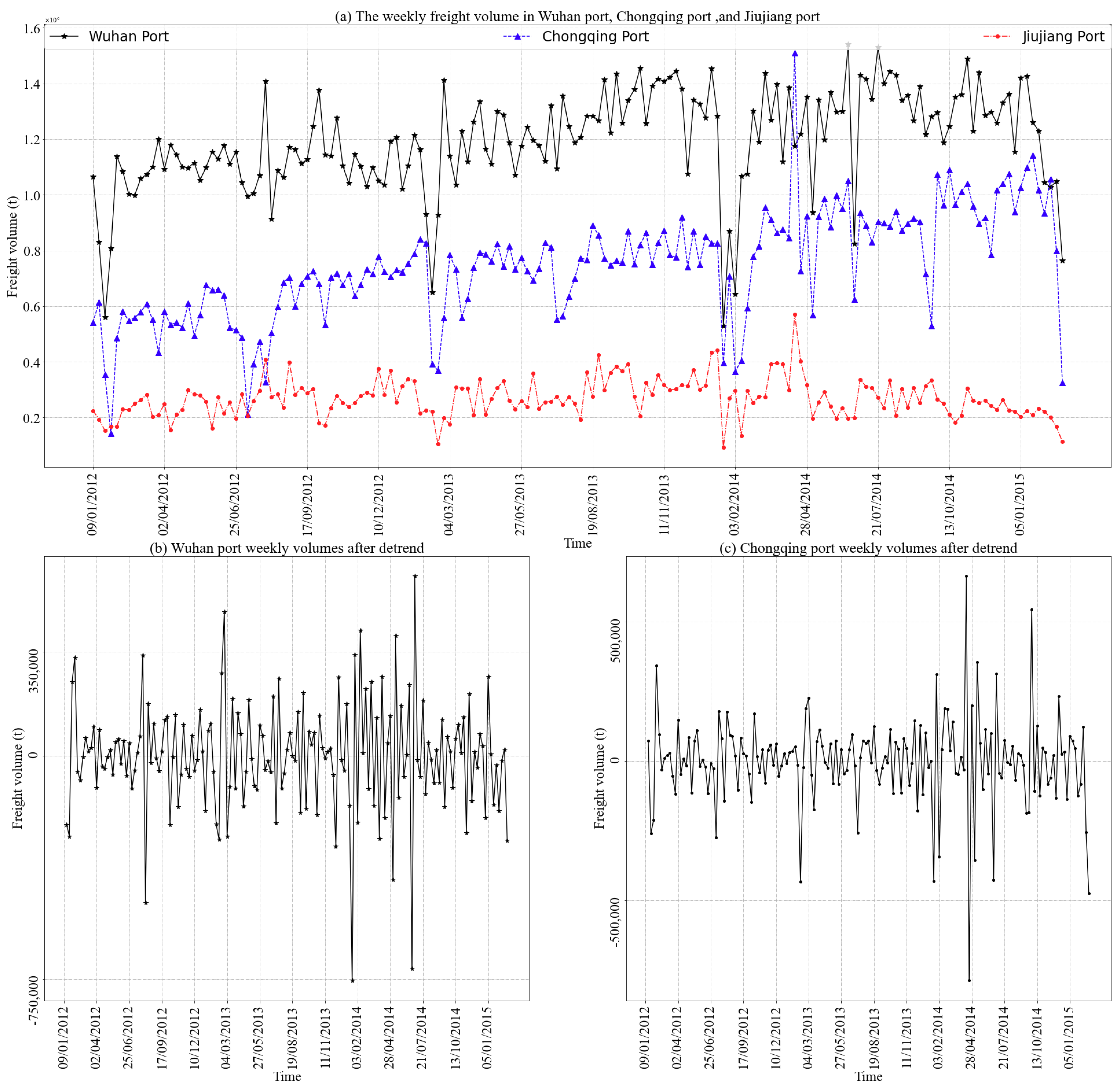
3.1.1. Port Locations and Freight Volume Data

Due to limited data availability, 12 ports in the main channel of the Yangtze River were selected as research objects. The locations of all these ports are shown in Figure 1. From upstream to downstream of the Yangtze River, they are: Chongqing Port, Yichang Port, Shashi Port, Chenglingji Port, Wuhan Port, Huangshi Port, Fuchi Port, Wuxue Port, Jiujiang Port, Hukou Port, Tongling Port, and Wuhu port, respectively. It can be seen that most of them are located in the middle of the Yangtze River.

The time scope of the freight volume data was from 0:00 on 2 January 2012 to 0:00 on 23 February 2015. The period from 0:00 on each Monday to 24:00 on each corresponding Sunday was recorded as one week, and thus there is a total of 164 weeks’ data.

Table 1. Port information and freight volume statistics.

Port	Province/ City	Distance from Wuhan Port (km)	Average Freight Volume per Week (t)	Average Freight Volume per Year (t)	Rank
Chongqing Port	Chongqing	1286	743,147.4	31,168,095.0	5
Yichang Port	Hubei	626	231,196.2	9,781,418.3	9
Shashi Port	Hubei	478	87,369.9	5,681,884.9	10
Chenglingji Port	Hunan	231	1,290,178.1	57,570,284.1	2
Wuhan Port	Hubei	0.0	1,194,259.3	57,803,446.1	1
Huangshi Port	Hubei	133	240,774.6	9,994,258.5	8
Fuchi Port	Hubei	195	55,721.4	988,158.1	12
Wuxue Port	Hubei	204	132,642.0	3,566,179.7	11
Jiujiang Port	Jiangxi	250	269,118.6	13,426,721.4	6
Hukou Port	Jiangxi	260	264,441.0	12,746,637.7	7
Tongling Port	Anhui	496	878,022.6	45,468,097.5	3
Wuhu Port	Anhui	600	691,657.1	38,161,639.8	4

shows more detailed information about each port and its corresponding freight volume. It is noted that distance is always used as a measure when characterizing the intensity of the relationship between ports [6,24]. Therefore, we calculated the channel route distance between Wuhan Port and each of the other ports based on its middle location in the Yangtze River channel. In addition, these ports were ranked according to their average freight volume per year in order to analyze whether there is was a relationship between spatial-temporal dependence and port grade.

3.1.2. Trend Analysis and Stationary Detection

To understand the trend of freight volume data, we drew a curve to represent the weekly freight volumes. Figure 2a shows the weekly freight volume curves of Wuhan Port, Chongqing Port, and Jiujiang Port. On the whole, the weekly freight of Wuhan Port and Chongqing Port showed a small increase while that of Jiujiang Port showed no obvious change. On the other hand, the curves fluctuated greatly from about January to February every year. This period corresponds to the Spring Festival in China, when most enterprises and workers take vacations, resulting in a sharp drop in freight volume.

Another important aspect is to ensure the stability of the time series when performing time series forecasting, especially for ARIMA [18] and SARIMA [15]. Stationary detection methods include autocorrelation, partial correlation, and the Augmented Dickey-Fuller test (ADF). This last test is more objective because it judges the existence of the unit root. Therefore, ADF was used to detect the stationary of freight cargo volume data. The results showed that the time series of most ports are stable, except for Yichang Port, Shashi Port, and Wuhu Port.

In order to eliminate the increasing trend of freight volume and keeping the stability of time series, all the freight volume data were detrended. Based on this step, we also hoped to analyze whether detrending processing helps to improve the forecasting performance of machine learning methods through the experiments detailed in Section 4. The difference method was adopted in order to eliminate trends in this paper. Furthermore Figure 2b,c show the curves of Chongqing Port and Wuhan Port after detrending the time series. It can be seen that the freight volume data of the two ports fluctuated around 0, and there was no growth trend.

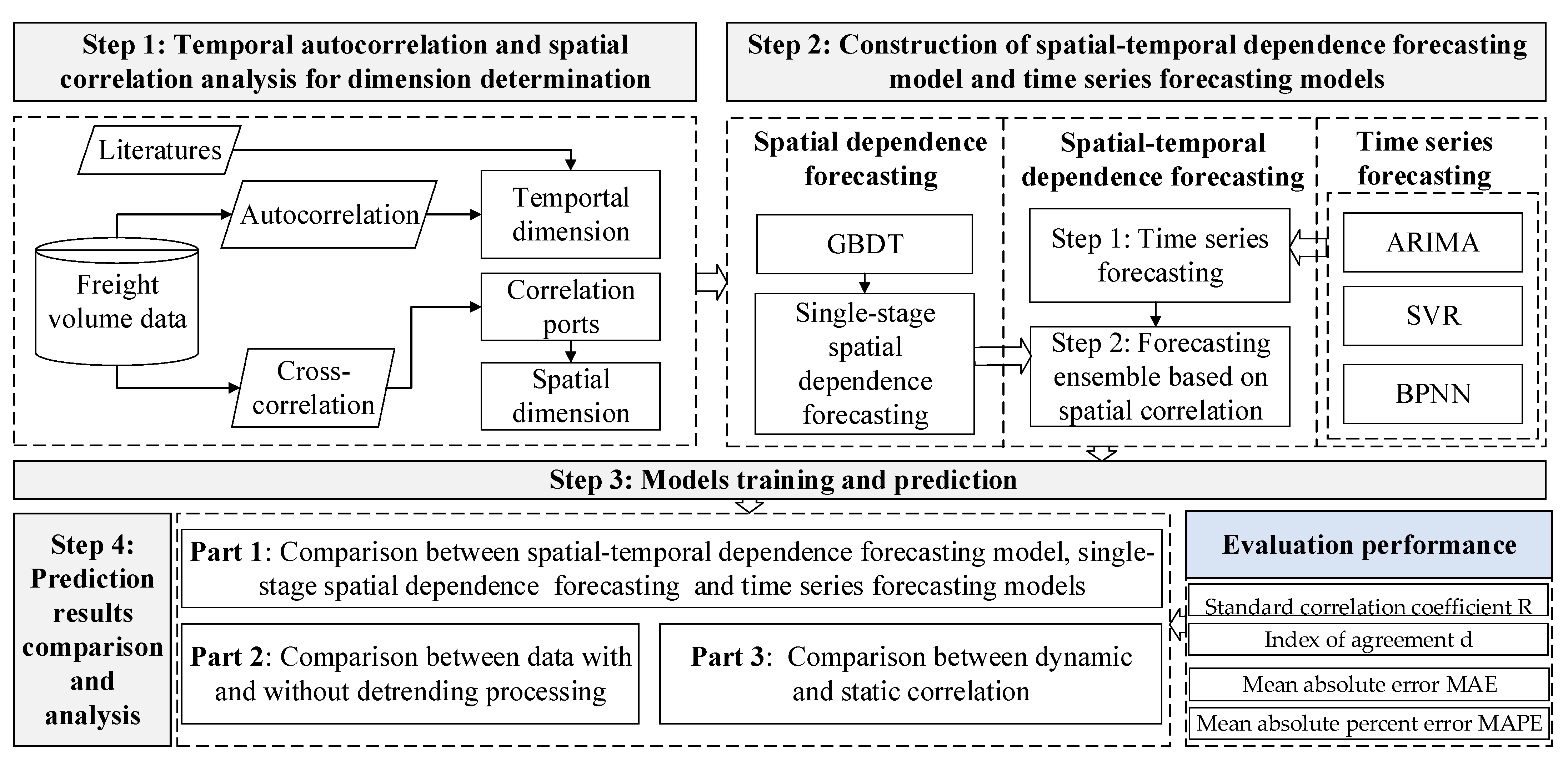
3.2. The Framework for Spatial-Temporal Dependence Forecasting and Analysis

The logical framework for spatial-temporal dependence forecasting and analysis is shown in Figure 3. It consisted of four main parts: a correlation analysis between freight volume data, the construction of spatial-temporal dependence and time series forecasting models, data partitioning and model training, and the prediction results from the comparison and analysis.

3.2.1. Correlation Analysis of Freight Volume Data

The correlation analysis of the freight volume data included the data autocorrelation analysis of a single port and the data cross-correlation analysis of different ports. The autocorrelation analysis was used to determine the temporal dimension $\delta$ (autoregressive window) in Formula (3), whereas the latter analysis was used to obtain the correlation between the port freight volume and the spatial dimension $m$ in Formula (3).

3.2.2. Autocorrelation Analysis

The freight volumes displayed periodicity with day [12] and season [15] as the grain size, respectively. In addition, Ruiz-Aguilar et al. [11] point out that although the prediction result will improve with the increasing size of the autoregressive window, the improvement will reduce with each increment of the size of the autoregressive window, up to a point of 21 days in the past, which implies that $\delta =3$ (weeks) may be a good choice. We verified this value through further experiments.

Spectrum analysis and autocorrelation analysis are usually used in periodic detection [47]. Spectrum analysis assumes that there is a period in the time series, whereas there is no such assumption in autocorrelation analysis. There was no clear periodic pattern in the port weekly freight volume data. Therefore, autocorrelation analysis was used in this paper. The autocorrelation function judges the correlation of time series by analyzing the similarity between the current value and the value with different lag $k$, as shown in Formula (1) [48]:

$$\mathrm{r}\left(k\right)=\frac{{{\displaystyle \sum }}_{i=1}^{n-k}\left(x_i-\overline{x}\right)\left(x_{i+k}-\overline{x}\right)}{{{\displaystyle \sum }}_{i=1}^n{\left(x_i-\overline{x}\right)}^2}$$

(1)

where $x_i$ is the measurement at time $i$ and $\overline{x}$ is the mean value.

3.2.3. Cross-Correlation Analysis

As mentioned in Section 2.1, the Pearson correlation was firstly used to obtain the overall relationship between the freight volumes of different ports. However, this method still did not provide insights into series dynamics. It would be better to know the leader–follower relationship in different time series when constructing the forecasting model. For example, if the freight volume of port X increases in this stage, resulting in the rise of freight volume at port Y in the next stage, then port X could be considered in the forecasting model for freight volume of port Y. Thus, we also used time-lagged cross-correlations (TLCC), which can identify directionality between double-time series. If the peak value of the relation curve is located in the center (that is, the offset is 0), the double-time series are synchronized at that time. The model definition of TLCC is similar to autocorrelation, as shown in Equation (2):

$$\begin{gathered} {\mathrm{g}}_k^{xy}=\frac{1}{n}{{\displaystyle \sum }}_{t=0}^{n-k}\left(y_t-\overline{y}\right)\left(x_{t+k}-\overline{x}\right) \\ {\mathrm{r}}_k^{xy}=\raisebox{1ex}{${\mathrm{g}}_k^{xy}$}\!\left/ \!\raisebox{-1ex}{$\sqrt{S{D}_x\times S{D}_y}$}\right. \end{gathered}$$

(2)

where $S{D}_x$ and $S{D}_y$ represent the standard deviation of series X and Y, and ${\mathrm{r}}_k^{xy}$ is the cross-correlation coefficient with the lag $k$ between them.

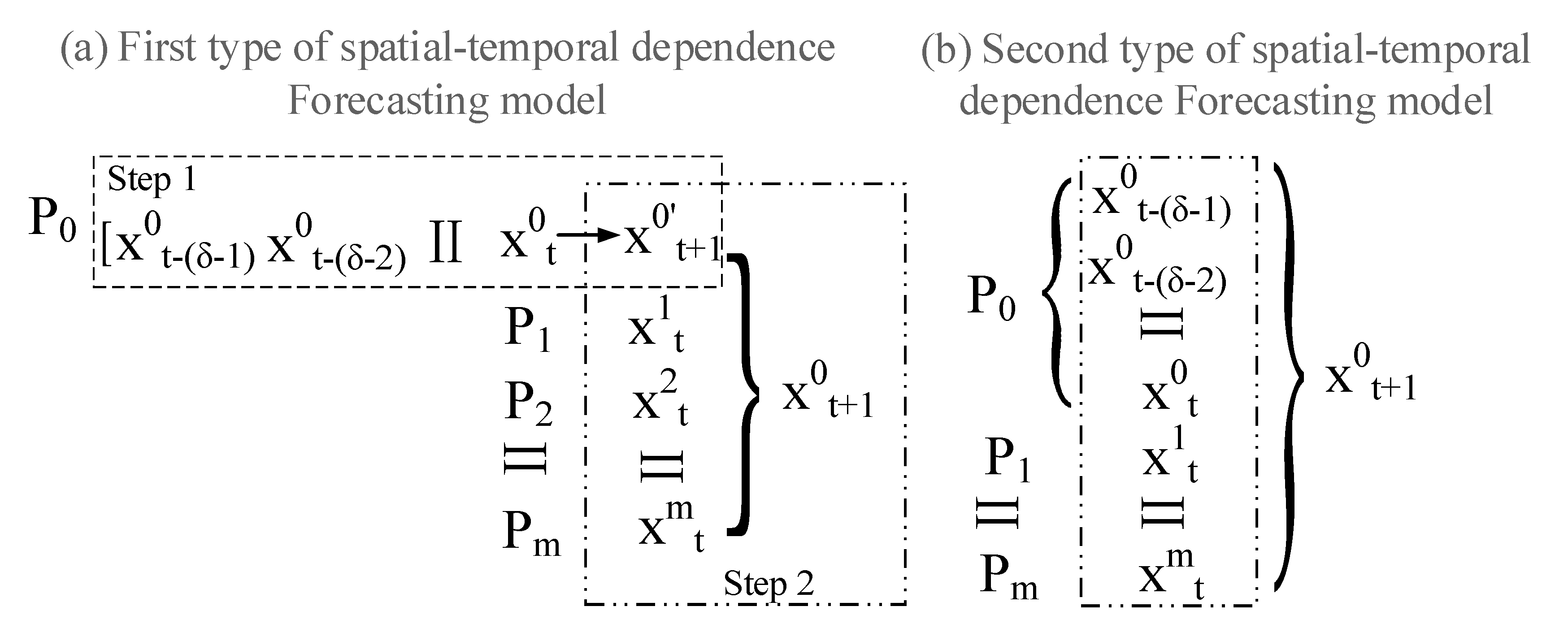
3.2.4. Spatial-Temporal Dependence Forecasting Model for Port Freight Volumes

The prediction based on the spatial-temporal dependence model can be seen as a function of multiple time serie, except it considers the relationship between the freight volumes of different ports. The ports whose freight volume has a spatial correlation with the target port $P_0$ are $P=\left\{P_1,P_2,\cdots ,P_m \right\}$, and $x_t^i$($i\in \left[0,m\right]$) represents the freight volume of $i_{th}$ the port at the period of $t$. In particular, $i=0$ indicates the target port. The spatial-temporal dependence forecasting model can be expressed as follows:

$$x_{t+1}^0=F\left(\left[\begin{array}{ccc}{x}_{t-\left(\delta -1\right)}^1& \dots & x_t^1\\ \begin{array}{c}⋮\\ x_{t-\left(\delta -1\right)}^m\end{array}& \begin{array}{c}\ddots \\ \dots \end{array}& \begin{array}{c}⋮\\ x_t^m\end{array}\\ x_{t-\left(\delta -1\right)}^0& \dots & x_t^0\end{array}\right]\right)$$

(3)

The model was further separated into two steps: the first was to obtain the forecasting of the time series, as in Step 1 in Figure 4a; the next was to obtain the final prediction combining the multiple forecasting results from Step 1 with the original data from other related ports, as in Step 2 in Figure 4a. The essential idea was to modify the time series predictions through a spatial forecasting model. The other option was to directly take the data of port $P_0$ and other ports as the input features of the forecasting model, as shown in Figure 4b.

Some forecasting methods for the time series are described in detail in Section 3.2.3, and the best forecasting model was used for Step 1 in Figure 4a, according to the comparison between the corresponding forecasting results in Section 4.2.1. On the other hand, we used the GBDT to complete the forecasting for Step 2 in Figure 4a. Its role in the freight volume forecast is analyzed below.

3.2.5. GBDT Forecasting Process

GBDT improves decision-making results by adding models (the linear combination of basic functions) and continuously reducing the residuals generated by the training process. Combined with Step 2 in Figure 4, the forecasting process for the freight volume of target ports was analyzed as follows:

• We calculated the average of $\left[x_{t+1}^1,x_{t+1}^2,\cdots ,x_{t+1}^m,x_{t+1}^0{}^{\prime }\right]$ as the initial learner $f_0\left(x\right)$;
• We calculated the residuals $r_i=-\left[\frac{\partial L\left({\left(x_{t+1}^0\right)}_i,f\left({\left[x_{t+1}^1,x_{t+1}^2,\cdots ,x_{t+1}^m,x_{t+1}^0{}^{\prime }\right]}_i\right)\right)}{\partial f{\left(\left[x_{t+1}^1,x_{t+1}^2,\cdots ,x_{t+1}^m,x_{t+1}^0{}^{\prime }\right]\right)}_i}\right]$, where $L$ is the lost function, and $\left({\left[x_{t+1}^1,x_{t+1}^2,\cdots ,x_{t+1}^m,x_{t+1}^0{}^{\prime }\right]}_i,{\left(x_{t+1}^0\right)}_i\right)$ is the $i_{th}$ training data;
• We built a tree with a goal of predicting the residuals, which takes $\left(\left[x_{t+1}^1,x_{t+1}^2,\cdots ,x_{t+1}^m,x_{t+1}^0{}^{\prime }\right],r_i\right)$ as the training data of the new tree;
• We calculated the best-fitting value ${\gamma }_j=\underset{\gamma }{\underbrace{argmin}}{\displaystyle \sum }_{y_i\in R_j}L\left(x_i,f\left(y_i\right)+\gamma \right)$ for leaf node area $R_j,j=1,2,\cdots ,J$, where $J$ is the number of leaf nodes of the tree;
• We updated $f\left(x\right)$ with $f\left(x\right)=f\left(x\right)+{{\displaystyle \sum }}_{j=1}^J{\gamma }_i$;
• We repeated step 2 to step 4 until the number of iterations $n$ matches the number specified by the hyperparameter;
• We used the last $f\left(x\right)$ to make a final prediction $x_{t+1}^0$ as to the value of the freight volume of the target port.

3.2.6. The Single-Stage GBDT Forecasting Model

The freight volume of the target port at $t+1$ can be forecasted through GBDT only based on their own data and those of correlated ports at $t$. In this way, $\left[x_{t+1}^1,x_{t+1}^2,\cdots ,x_{t+1}^m,x_{t+1}^0{}^{\prime }\right]$ in Step 2 in Figure 4 could be replaced by $\left[x_{t+1}^1,x_{t+1}^2,\cdots ,x_{t+1}^m,x_{t+1}^0\right]$, and Step 1 in Figure 4 could be omitted. We also carried out experiments in order to analyze the effectiveness of the spatial-temporal dependence forecasting model and the single-stage GBDT forecasting model.

3.3. Time Series Forecasting Models of Port Freight Volumes

Through implementing time series forecasting, we were able to determine whether the spatial-temporal dependence model was better by comparison. On other hand, the best time series model was used for Step 1 in Figure 4. Formula (4) depicts the model of time series forecast for freight volumes [11]; the parameters are introduced above.

$$x\left(t+1\right)=F\left\{x\left(t\right),x\left(t-1\right),\cdots ,x\left(t-\left(\delta -1\right)\right)\right\}$$

(4)

According to Section 2.2, the neural network and support vector regression generally performed better than other machine learners in freight volume forecasts. In addition to the machine learning methods, the traditional method, ARIMA model, was also selected as a model for comparison.

3.3.1. Auto-Regression Integrated Moving Average

The ARIMA model consists of an AR model and an MA model, as shown in Formula (5). The AR model, which requires that the time series be stationary and that it has a certain autocorrelation, is used to describe the relationship between the current value and the historical value. The MA model illustrates the accumulation of error terms in the autoregressive model to eliminate the random fluctuation in prediction:

$$x_{t+1}=\mu +{{\displaystyle \sum }}_{i=1}^{\delta }{\gamma }_i{x}_{t-\left(i-1\right)}+{\epsilon }_{t+1}+{{\displaystyle \sum }}_{i=1}^q{\theta }_i{\epsilon }_{t-\left(i-1\right)}$$

(5)

where $\mu$ is a constant term, whereas ${\mathsf{\epsilon }}_{t+1}$ is an error term, ${\gamma }_i$ and ${\theta }_i$ are coefficient, and the parameters $\delta$ and $q$ need to be determined based on the Bayesian Information Criterion (BIC). In addition, the time series need to be converted into stationary series by different methods, which are described in Section 3.1.2. Therefore, the construction process of the ARIMA model includes: (a) the conversion of the time series into into stationary sequences; (b) the determination of the parameters $\delta$ and $q$; (c) the construction of the ARIMA model in order to perform forecasts according to the parameters.

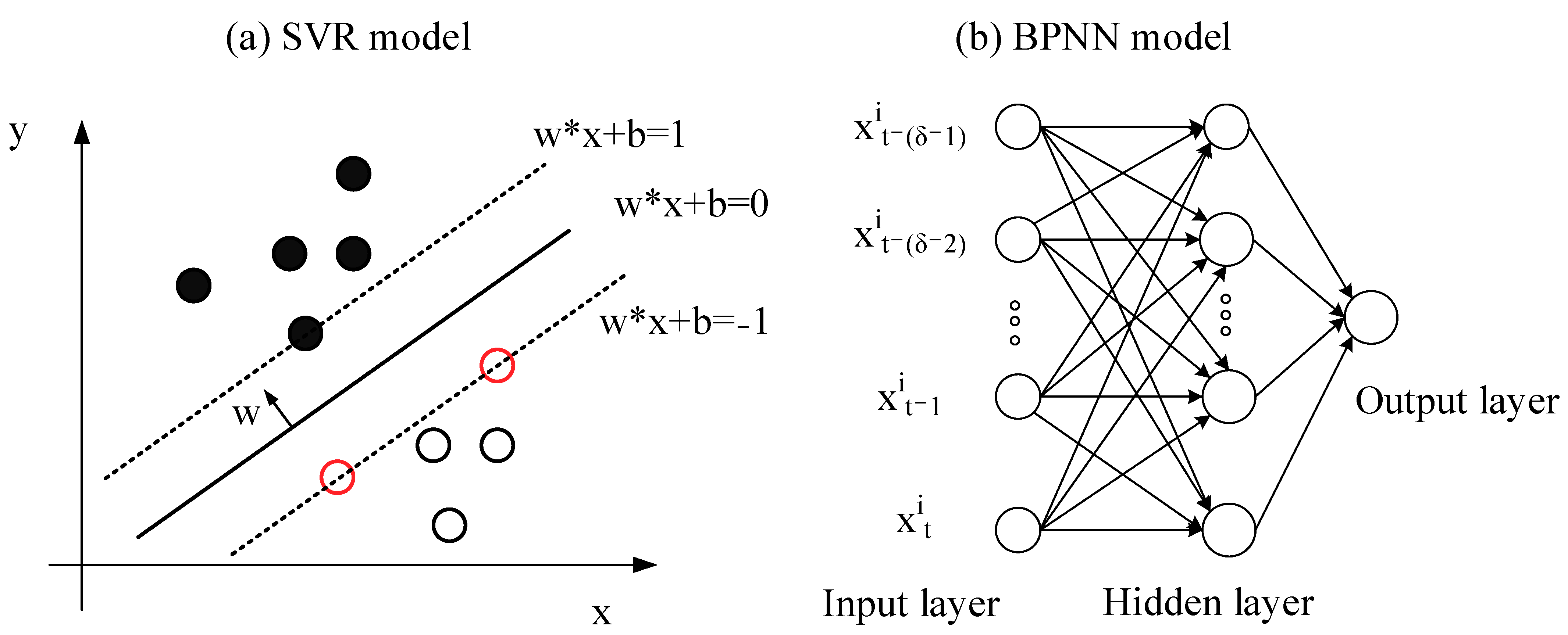
3.3.2. Support Vector Regression

SVR is always used in prediction and performs well [17,49]. The kernel function further promotes prediction accuracy [50]. As shown in Figure 5a, SVR combines the support vector machine (SVM) and regression methods, and thus it still features the characteristics of SVM, which means that the loss is calculated only if the difference between the predicted value and the actual value is greater than $\epsilon$. The goal of SVR is to minimize forecasting errors and to maximize the interval between two margins that are parallel to the hyperplane. If the expression of the hyperplane is $f\left(x\right)=w^{T}x+b$, then the objective function is as follows:

$$\underset{w,b}{\min }\frac{1}{2}{\Vert w\Vert }^2+C{{\displaystyle \sum }}_{i=1}^m{l}_{\epsilon }\left(f\left(x_i\right)-y_i\right)$$

(6)

where ${\mathrm{l}}_{\epsilon }\left(z\right)=\left\{\begin{array}{c}0, if \left|z\right|\le \epsilon \\ \left|z\right|-\epsilon , otherwize\end{array}\right.$ and $C$ is the regularization constant, and $\left(x_i,y_i\right), i\in \left(1,m\right)$ represents the training data. If the samples cannot be fitted by the linear model, the original space needs to be mapped into high-dimensional space. The kernel functions, such as linear kernel function and polynomial kernel function, are always used in SVR. Generally, SVR for forecasting includes the following four steps:

(a)

data standardization to prevent local features from being too large or too small, and to speed up the calculation;

(b)

the determination of the kernel function and the parameters $C$, and the construction of the SVR model;

(c)

training of the SVR model based on training data;

(d)

the prediction of the target value after obtaining the model.

3.3.3. Back-Propagation Neural Network

Although deep learning methods, especially long-short term memory (LSTM) networks, are able to capture the features of time series over a longer time span [51,52,53], the 21 days (three weeks) is an appropriate autoregressive window, and neural networks perform better than any other model independently of the size of the autoregressive window [11]. Therefore, BPNN is still used for comparison research instead of LSTM. As shown in Figure 5b, BPNN includes the input layer, the hidden layer, and the output layer. The whole BPNN consists of many neural units, and each neural unit can be represented as:

$$y=f\left({{\displaystyle \sum }}_{i=1}^n{w}_i{x}_i+b\right)$$

(7)

where $x_i$ is the input of the current neural unit, $w_i$ is the connecting weight, $b$ is the threshold, and $f$ is the activation function. Unlike other neural networks, BPNN updates weights and thresholds by minimizing the errors between predicted and true values. The processes, which are similar to those in SVR, include: (a) data standardization; (b) the structural determination of BPNN and the initialization of weights and thresholds; (c) updating the parameters through a back-propagation algorithm based on training data; (d) the prediction of the target value after obtaining the model.

3.3.4. Evaluation Methods for Forecasting Results

There are several statistical methods available to evaluate forecast performance [17], including the standard correlation coefficient $\mathrm{R}$, the index of agreement $\mathrm{d}$, mean absolute error $\mathrm{MAE}$, and mean absolute percent error $\mathrm{MAPE}$, as follows:

$$\mathrm{R}=\frac{{{\displaystyle \sum }}_{i=1}^N\left(y_i-\overline{y}\right)\left(x_i-\overline{x}\right)}{\sqrt{{{\displaystyle \sum }}_{i=1}^N{\left(y_i-\overline{y}\right)}^2{{\displaystyle \sum }}_{i=1}^N{\left(x_i-\overline{x}\right)}^2}}$$

(8)

$$\mathrm{d}=1-\frac{{{\displaystyle \sum }}_{i=1}^N{\left(y_i-x_i\right)}^2}{{{\displaystyle \sum }}_{i=1}^N{\left(\left|y_i-\overline{x}\right|+\left|x_i-\overline{x}\right|\right)}^2}$$

(9)

$$\mathrm{MAE}=\frac{1}{N}{{\displaystyle \sum }}_{i=1}^N\left|y_i-x_i\right|$$

(10)

$$\mathrm{MApE}=\frac{100}{N}{{\displaystyle \sum }}_{i=1}^N\frac{\left|y_i-x_i\right|}{x_i}$$

(11)

where $x_i$ and $y_i$ are the true and predicted values, $\overline{x}$ and $\overline{y}$ are the corresponding average values, and $N$ is the number of samples. Notably, $\mathrm{R}$ and $\mathrm{d}$ close to 1 performed better, whereas lower $\mathrm{MAE}$ and $\mathrm{MAPE}$ indicated overperformance.

3.4. Experimental Design

To ensure the stability and accuracy of the predictions, the strategy of dataset partitioning and parameter selection for obtaining models were considered.

3.4.1. Dataset Partitioning

Common cross-validation procedures can be adapted for time series prediction evaluation when autoregressive models are used [54]. Therefore, the K-fold cross-validation was performed on the time series. As mentioned in Section 3.1, there was a total of 164 weeks’ data on multiple ports, therefore the analysis was carried out by performing 5-fold cross-validation. In this sense, the models were fitted in four folds (train set) and tested in the left fold. This procedure can be repeated 20 times to guarantee the randomness of the partitioning process [11]. However data partitioning is not suitable for ARIMA, and thus we used the detrended data directly for training and testing, while keeping the data size the same as for the machine learning methods.

3.4.2. Parameter Selection

It is important to select suitable parameters for machine learning models to create accurate predictions. Generally, there are three methods of parameter adjustment in machine learning, namely, grid search, random search, and Bayesian optimization. Grid search offers reliable results but it is too slow, while random search is fast but important points may be missed in the search space. Therefore, Bayesian optimization was adopted for this paper. The optimization results were different for each data random division process; we took the mean values of the continuous variables and the modes of the discrete variables.

Specifically, grid search is applicable in ARIMA due to the limitation on $\delta$ and $q$. As for BPNN, the number of layers is set 3 and the number of neurons of the middle layer can be determined as follows:

$$N_h=\frac{N_s}{\alpha \ast \left(N_i+N_o\right)}$$

(12)

where $N_i$ is the number of neurons in the input layer, $N_o$ is the number of neurons in the output layer, $N_s$ is the number of training samples, and $\alpha$ is always selected between 2 and 10. In this way, we were able to set the scope of the number of neurons in the middle layer when using Bayesian optimization.

4. Results

This section contains the correlation analysis of port freight volumes and the comparison between the predictions of different models.

4.1. Correlation Analysis of Port Freight Volume

The autocorrelation analysis of the port weekly freight volume data and the correlation analysis between the weekly freight volume data of different ports can not only help to understand the actual weekly freight volume of inland ports but it can also be used to determine parameters for the forecasting models.

4.1.1. Autocorrelation Analysis of Port Freight Volume

Generally, the weekly freight volume of a specific port has a stronger correlation with that of the previous few weeks [11]. Therefore, all the data from 2012 to 2014 were divided into 13 segments, and each segment contained 12 weeks (approximately a quarter’s worth) of data. The temporal correlation between the last week and the first 11 weeks of freight volume in each segment was analyzed. Figure 6 shows the weekly autocorrelation results of the different grades. The horizontal axis 0 represents the current week, the horizontal axis $i$ represents the previous week, and the vertical axis represents the date of the current Sunday.

It can be seen that:

(a)

There was no obvious periodic pattern in the time series of weekly freight volume;

(b)

With the increase of the time interval between the current week and the previous week, the correlation decreased gradually;

(c)

The weeks with higher correlation are the antecedent 1–3 weeks, but there is both positive and negative autocorrelation.

In addition, there were few differences between the freight volume autocorrelation results of different ports. For example, the proportion of positive correlation to negative correlation was basically the same in the previous 1–2 weeks for Wuhan Port. However, the weekly freight volume in the past week mainly showed a positive correlation for Chongqing Port, while that in the previous 2 weeks mainly showed a negative correlation. For Shashi Port, the previous 1–2 weeks mainly showed a positive correlation.

Compared with the freight volume autocorrelation, with a quarter as the time granularity [6], the current freight volume only showed a strong correlation with the freight volume of the previous 1–2 stages. Therefore, we also determined $\delta =3$ according to Ruiz-Aguilar’s conclusion [11].

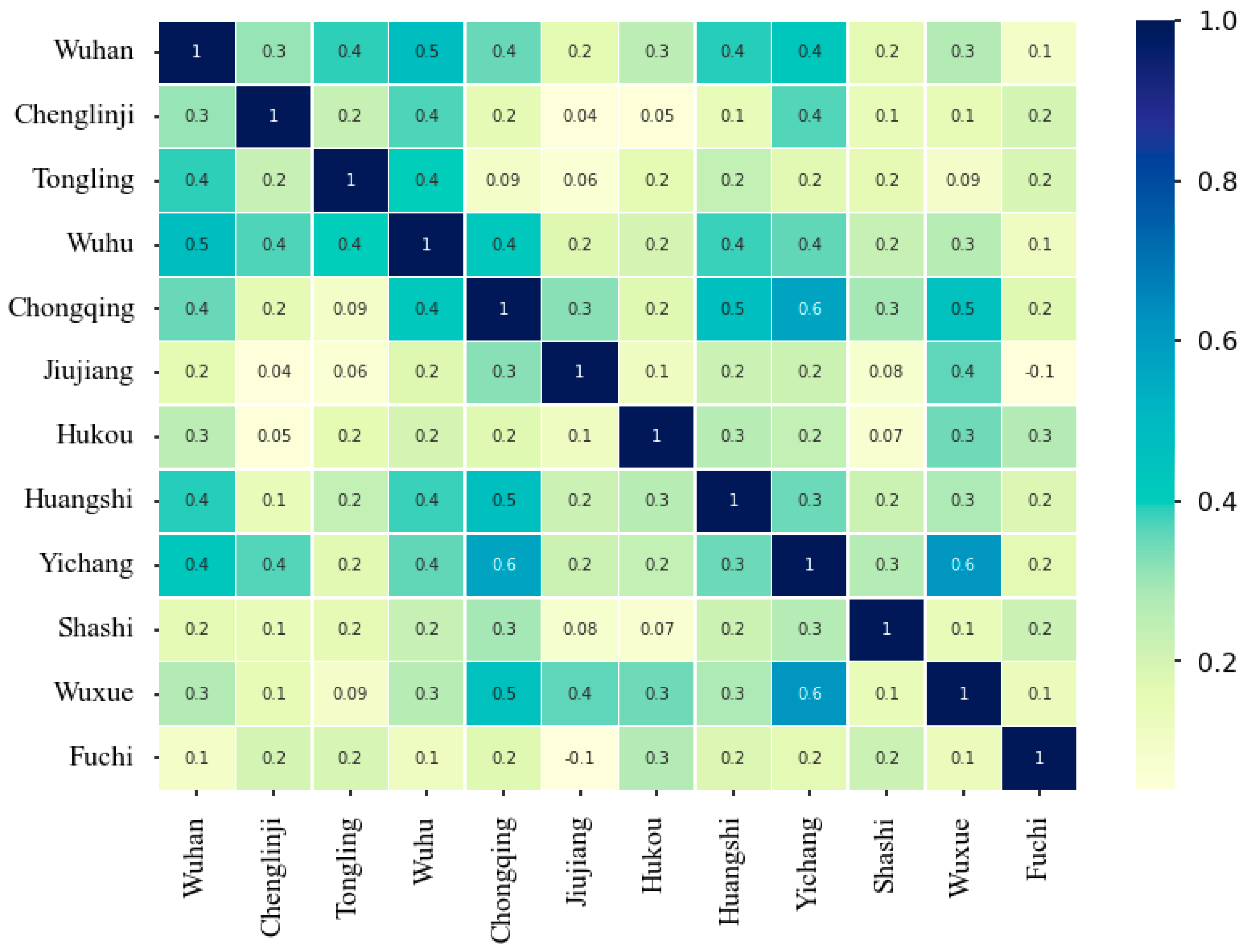
4.1.2. Freight Volume Correlation Analysis between Ports

The Pearson correlation was first used to carry out primarily correlation analysis, as shown in

Table 2. Pearson correlation coefficient matrix of port freight volumes.

	1	2	3	4	5	6	7	8	9	10	11	12
1	1	0.572	0.293	0.157	0.353	0.464	0.173	0.457	0.321	0.173	0.094	0.425
2	0.572	1	0.266	0.367	0.432	0.347	0.164	0.615	0.219	0.237	0.169	0.356
3	0.293	0.266	1	0.139	0.164	0.219	0.221	0.139	0.079	0.068	0.152	0.230
4	0.157	0.367	0.139	1	0.308	0.141	0.203	0.148	0.040	0.0490	0.227	0.370
5	0.3523	0.432	0.164	0.308	1	0.392	0.095	0.271	0.160	0.254	0.390	0.473
6	0.464	0.347	0.219	0.141	0.392	1	0.185	0.280	0.221	0.265	0.237	0.384
7	0.173	0.164	0.221	0.203	0.095	0.185	1	0.130	−0.108	0.270	0.190	0.113
8	0.457	0.615	0.139	0.148	0.271	0.280	0.130	1	0.360	0.345	0.092	0.262
9	0.321	0.219	0.079	0.040	0.160	0.220	−0.108	0.360	1	0.114	0.060	0.175
10	0.173	0.237	0.068	0.0490	0.254	0.265	0.269	0.345	0.114	1	0.160	0.201
11	0.094	0.169	0.152	0.227	0.390	0.237	0.190	0.092	0.060	0.160	1	0.402
12	0.425	0.356	0.230	0.370	0.473	0.384	0.113	0.262	0.175	0.201	0.402	1

. Most correlations between the ports’ weekly freight were positive, but there was a negative correlation between Fuchi Port and Jiujiang Port. The highest Pearson correlation value of the ports’ weekly freight volume was 0.615, and the Pearson correlation values were mainly distributed between 0.2 to 0.5, which account for 50% of the total. In addition, the highest Pearson correlation values (bold italic numbers) in more rows did not tend to approach the diagonal of the matrix, indicating that there seemed not to be a higher correlation between the weekly freight volume of ports located close to each other; we numbered the ports from the upstream to downstream of Yangtze River.

The numbers from 1 to 12 indicate Chongqing Port, Yichang Port, Shashi Port, Chenglingji Port, Wuhan Port, Huangshi Port, Fuchi Port, Wuxue Port, Jiujiang Port, Hukou Port, Tonling Port, and Wuhu Port.

In addition to considering the overall relevance between port weekly freight volumes, we also paid attention to whether there was a lag between the ports’ weekly freight volumes, whether the correlation was related to the ports’ grades, and whether the relevance changed dynamically.

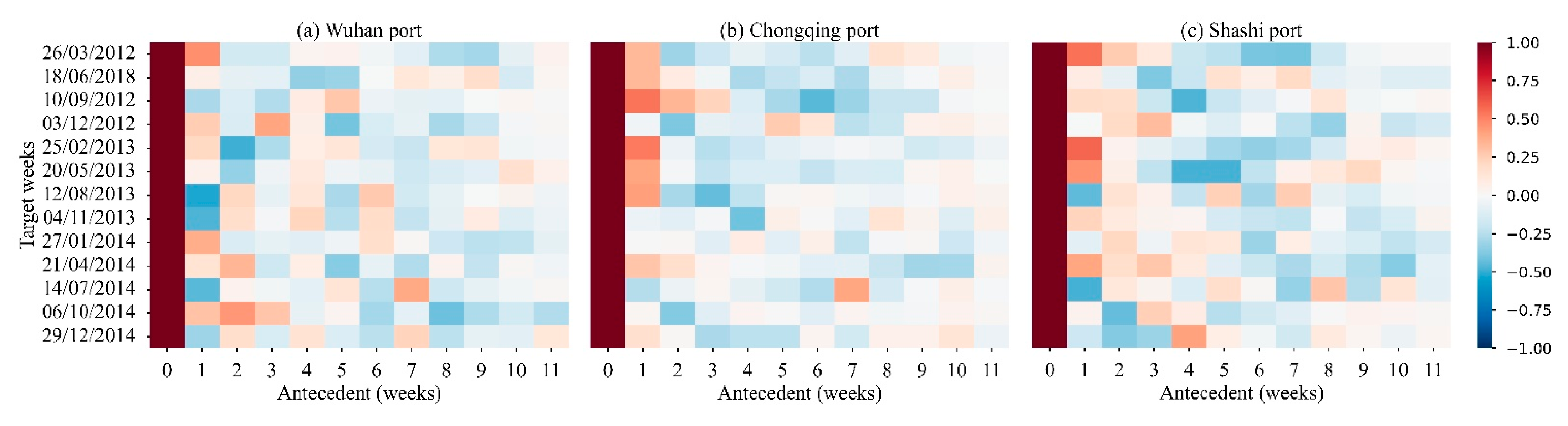
4.1.3. Was There a Lag between the Weekly Freight Volumes of Different Ports?

We tried to determine whether there was a lag between the weekly freight volumes in order to judge whether there was a guide-follow relationship between the different ports. We set the window size at 20 weeks and then used windowed time-lagged cross-correlations (WTLCC) based on Equation (2) to analyze the weekly freight volume of the target port and that of the other ports every month, as shown in Figure 7.

The freight volume correlations between these three ports and Wuhan Port were different. For example, although the main weekly freight volume correlations between the three ports and Wuhan Port were positive when the offset week was 0, the correlation between Chongqing Port and Wuhan was relatively continuous, while the correlations between Chenglingji Port, Shashi Port, and Wuhan Port were segmented. Generally, if there is a guide–follow relationship between two port freight volumes, it will mainly display negative (positive) values in the negative offset weeks while displaying positive (negative) values in the positive offset weeks. However, according to Figure 7, it seems that there was no such trend, except for Chenglingji Port, where the freight volume correlation with other ports remained unstable.

4.1.4. Is the Correlation of Ports’ Weekly Freight Volume Dynamic?

As shown in Figure 7, the freight volume correlations between specific ports and Wuhan Port changed dynamically. For example, the higher correlations between the freight volumes of Wuhan Port and Chenglingji Port were found in June 2012 and June 2014, while this was not the case for June 2013, which indicates that there was no periodic pattern of correlation between the freight volume of different ports. However, we could also consider the dynamic variation characteristics of correlation when carrying out the spatial-temporal correlation prediction.

4.1.5. Is the Correlation of Ports’ Weekly Freight Volume Related to Ports’ Grades?

To determine whether the correlation of weekly freight volumes was related to the ports’ grades, we changed the order of the volumes in Table 2 and displayed it through a heat map, as shown in Figure 8. It shows that ports with higher grades had a higher correlation of weekly freight volume with each other than with ports with a lower grade. In addition, Huangshi Port, Yichang Port, and Wuxue Port had a higher correlation with other ports.

Furthermore, the spatial dimension $m$ for the spatial forecasting model needed to be determined. The predictions of GBDT based on different $m$ dimensions were compared. Figure 9 shows that there was no obvious difference between different $m$ dimensions. To maintain consistency with the input dimensions of the time series predictions, we also set $m=3$, which meant that the weekly freight volume data of the three ports thathad the highest correlation with the target port were used as the input data for the spatial forecasting model, including the target port’s own freight volume data.

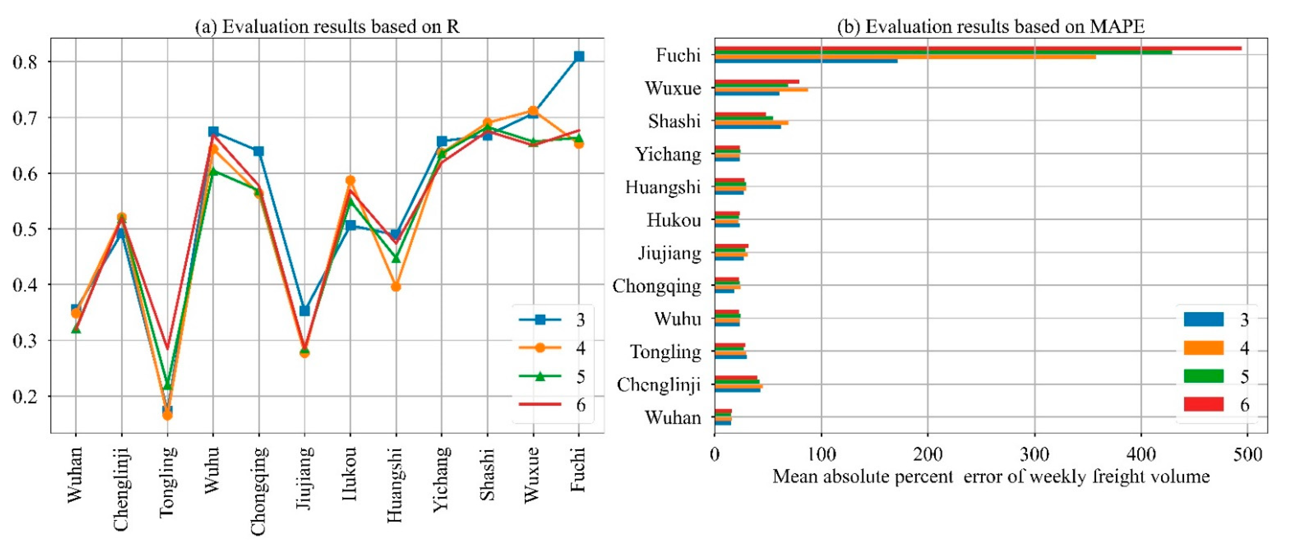
4.2. Prediction Comparison between Different Forecasting Models

This work aimed to verify whether the spatial-temporal dependence model can improve the forecasting of the short-term freight volume of inland ports. Therefore, we first carried out a forecast based on spatial-temporal dependence forecasting models and time series forecasting models, as discussed in Section 4.2.1. We then analyzed the effect of the dynamic correlation and the detrending process on spatial-temporal dependence forecasting, as discussed in Section 4.2.2 and Section 4.2.3, respectively.

As mentioned above, the hyper-parameters are important for machine learning methods, and Bayesian optimization was used to obtain suitable parameters.

Table 3. Hyper-parameters of freight volume forecasting models.

Ports	Models and Hyper-Parameters
	ARIMA		SVR		BPNN		GBDT
	$\mathit{\delta }$	$\mathit{q}$	$\mathit{C}$	Kernel	Activation	Number of Neurons	$\mathit{n}$ Estimators	Learning Rate	Max Depth
Chenglingli	2	0	8.01	linear	relu	7	97	0.0266	18
Chongqing	3	3	8.53	poly	relu	10	103	0.0012	21
Fuchi	0	1	5.43	rbf	tanh	5	95	0.0018	20
Huangshi	0	1	6.96	linear	tanh	9	97	0.0567	19
Hukou	0	1	7.52	linear	relu	9	99	0.0777	20
Jiujiang	1	0	12.28	linear	identity	8	103	0.0216	23
Shashi	0	2	5.06	rbf	relu	8	93	0.0315	22
Tongling	2	1	10.05	linear	relu	9	100	0.1166	21
Wuhan	2	0	9.2	rbf	tanh	9	99	0.1235	22
Wuhu	2	0	6.63	linear	tanh	7	98	0.1042	22
Wuxue	1	0	9.33	linear	relu	10	98	0.1672	20
Yichang	2	2	9.81	poly	relu	8	97	0.05378	18

shows the best hyper-parameters of four basic forecasting models when $\delta =3$ (for SVR, BPNN) and $m=3$ (for GBDT). The hyper-parameters were different for the weekly freight volume data of different ports. The hyper-parameters of subsequent models were determined by Bayesian optimization.

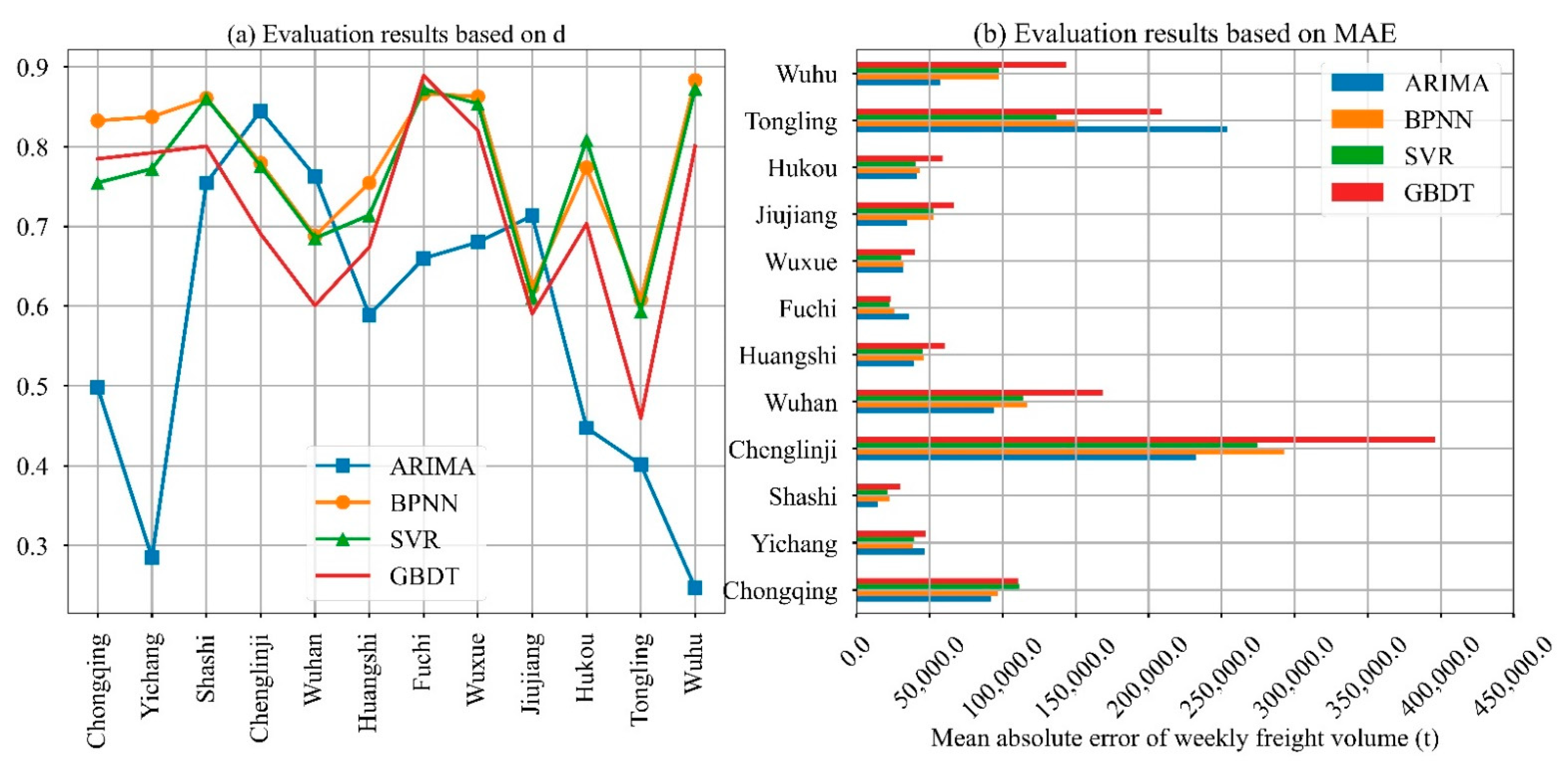
4.2.1. Comparison between Spatial-Temporal Dependence Forecasting and Time Series Forecasting

As shown in Figure 10, we used $\mathrm{MAE}$ and $\mathrm{d}$ to evaluate the prediction results based on the ARIMA, BPNN, SVR, and single-stage GBDT forecasting models. Figure 10a shows that the models with the most accurate and most stable predictions were BPNN and SVR, while the ARIMA model performed poorly. According to the $\mathrm{MAE}$ in Figure 10b, the single-stage GBDT forecasting model was not reliable, while SVR was more accurate than BPNN.

According to the evaluation analysis based on Figure 10, SVR was selected for spatial-temporal dependence forecasting models in Figure 4a, and noted as SVR-GBDT. In addition, the SVR was also deemed to be suitable for the construction of forecasting models based on Figure 4b, and noted as Sspatial-temporal SVR (STSVR). Consequently, the prediction results of SVR, SVR-GBDT, and STSVR, were compared, as shown in

Table 4. Evaluation results of predictions based on SVR, SVR-GBDT, and STSVR.

Ports	Models	$\mathit{R}$	$\mathit{d}$	$\mathit{M}\mathit{A}\mathit{E}$	$\mathit{M}\mathit{A}\mathit{P}\mathit{E}$
Chongqing Port	SVR-GBDT	0.6142	0.7645	114814	17.5140
	STSVT	0.6354	0.7793	109594	17.2641
	SVR	0.6271	0.7549	111383	17.1492
Yichang Port	SVR-GBDT	0.6318	0.7860	46907.8	23.0705
	STSVT	0.7110	0.8323	37346.2	18.8978
	SVR	0.6131	0.7723	39594.2	18.6422
Shashi Port	SVR-GBDT	0.6629	0.7979	27866.8	71.2912
	STSVT	0.7717	0.8652	20955.1	62.7795
	SVR	0.7619	0.8609	21156	52.5459
Chenglingji Port	SVR-GBDT	0.4909	0.6913	388887	43.795
	STSVT	0.6209	0.7776	295815	35.539
	SVR	0.6197	0.7759	274525	30.2371
Wuhan Port	SVR-GBDT	0.3544	0.6002	150934	14.3819
	STSVT	0.4212	0.6399	112476	11.1286
	SVR	0.4685	0.6852	114343	10.6734
Huangshi Port	SVR-GBDT	0.4383	0.6420	62257.2	20.0887
	STSVT	0.5985	0.7533	45119.9	20.1444
	SVR	0.5276	0.7141	45383	21.4577
Fuchi Port	SVR-GBDT	0.8013	0.8817	23504.5	124.399
	STSVT	0.7941	0.8727	24230.3	335.966
	SVR	0.7912	0.8724	22878.8	268.399
Wuxue Port	SVR-GBDT	0.6732	0.7971	43535.6	44.4348
	STSVT	0.7878	0.8699	29921.2	29.4547
	SVR	0.7589	0.8534	30449	32.8891
Jiujiang Port	SVR-GBDT	0.2311	0.5185	69281.1	28.7139
	STSVT	0.3651	0.6139	49234.8	20.9561
	SVR	0.3922	0.6107	52461.3	22.0805
Hukou Port	SVR-GBDT	0.4671	0.6751	62505.6	25.4328
	STSVT	0.6364	0.7829	43338.2	18.0239
	SVR	0.6780	0.8084	40370	16.5361
Tongling Port	SVR-GBDT	0.1231	0.4481	220966	30.5405
	STSVT	0.2423	0.5294	156148	24.1003
	SVR	0.3308	0.5934	137192	20.0258
Wuhu Port	SVR-GBDT	0.6333	0.7758	143389	23.1780
	STSVT	0.6627	0.7838	126290	20.5344
	SVR	0.7797	0.8729	97741.1	15.9640

.

As can be seen in Table 4, the prediction results of SVR and STSVR were better and similar, whereas the SVR-GBDT did not show good forecasting effectiveness. It seems that spatial-temporal correlation information helps in the performance of weekly freight volume forecasts for most inland ports (bold marker). However, the spatial-temporal dependence forecast models do not offer great improvements in the prediction of weekly freight volume.

4.2.2. Comparison between Static Spatial Dependence and Dynamic Spatial Dependence

Due to the complexity of the inter-port relationship [24] and its variability, as influenced by a range of factors [55], the spatial correlation of port freight volume is dynamic, as demonstrated by Figure 7. Therefore, we tried to construct new training data and test data corresponding to the dynamic cross-correlation results.

The specific steps were as follows. Firstly, the first 152 weeks’ data from each port were evenly separated into 38 segments, where each segment contained 10 weeks’ data, and the interval between the beginning of each segment was about one month. Subsequently, the weekly freight volume cross-correlation coefficient between each segment of each port was calculated according to Equation (2). Finally, according to the data stage of the target port and the cross-correlation results from the corresponding period, the data of the three ports with the highest correlations with the target port were chosen to build training sets and test sets. We inputted these datasets into SVR models, notated the dynamic STSVR, and compared the predictions with those of the static STSVR, as mentioned earlier.

As shown in Figure 11, according to the evaluation results based on $\mathrm{d}$ and $\mathrm{R}$, the dynamic STSVR performed better than the static STSVR for almost all ports except Wuxue Port. Furthermore, in addition to Jiujiang Port, Wuxue Port, and Huangshi Port, the dynamic STSVR also obtained better prediction results according to the evaluation results based on $\mathrm{MAE}$ and $\mathrm{MAPE}$. Therefore, although there was no great difference between static and dynamic STSVR, the dynamic SRSVR still offered improved predictions.

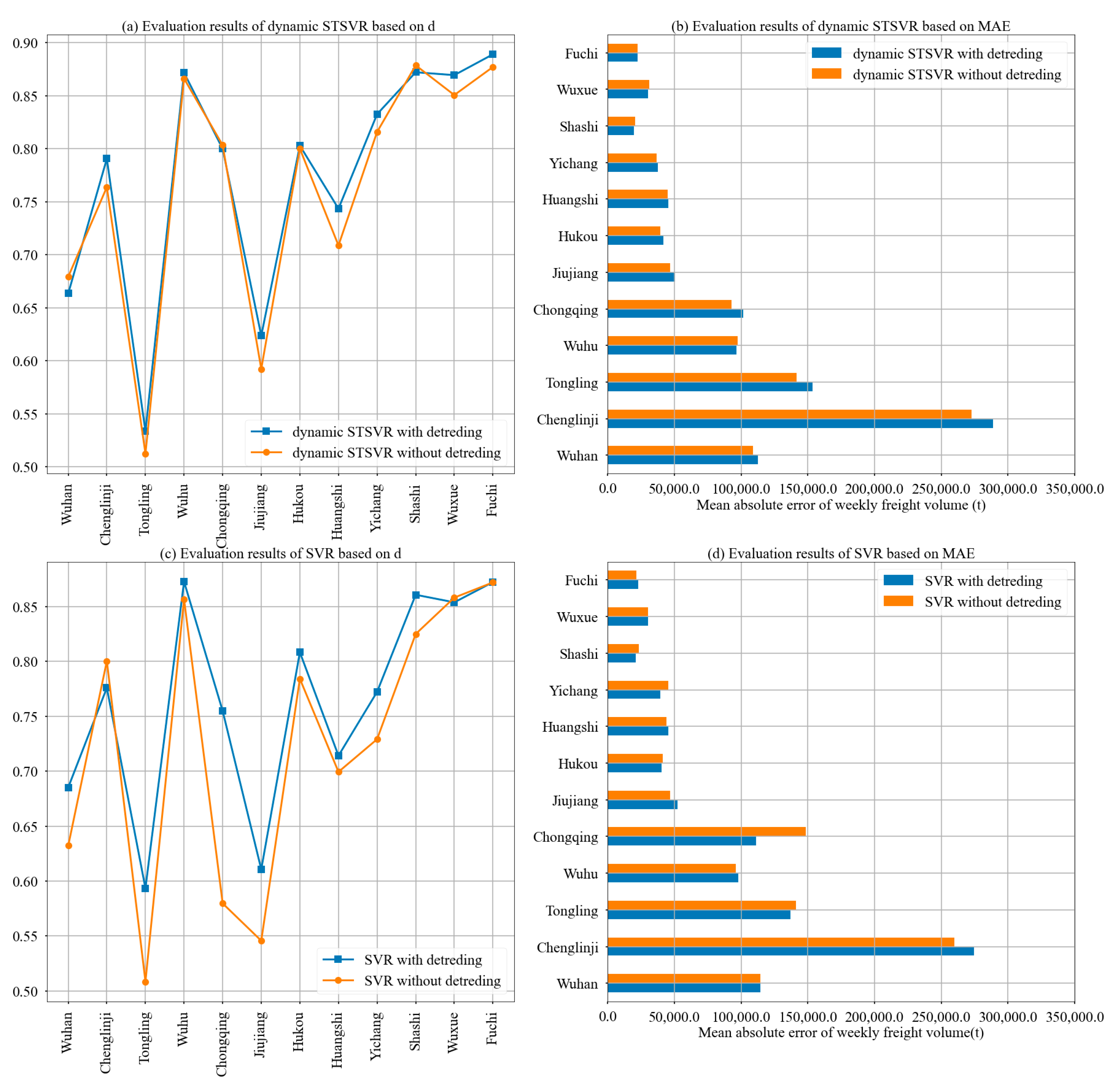
4.2.3. Comparison between Time Series with and without Stationary Processing

Although the question of whether stationary processing is significant for weekly freight volume forecasting is not the main goal of this work, it also plays an important role in the formation of accurate predictions. Thus, we also carried out experiments on the prediction comparison based on time series with and without stationary processing. The dynamic STSVR and the SVR for time series forecasting were selected for this comparison experiment.

By comparing Figure 12a with Figure 12c, we found that the prediction results based on data with stationary processing were generally better than those based on original data, and that the time series forecasts were more easily affected by the stationary processing. However, according to the evaluation results based on $\mathrm{MAE}$ Figure 12b,d, the dynamic STSVR method with detrending time series featured more errors, which was the opposite of the performance of the SVR model with detrending time series.

On the other hand, by combining Table 4 with Figure 12, we found that the spatial-temporal dependence models and the time series forecasting models performed similarly. If the prediction results based on SVR were good, the corresponding results based on spatial-temporal dependence models were also acceptable, and vice versa. This finding can be explained by the fact that forecasting results of ports are more dependent on their past data.

5. Discussion

This paper proposed a short-term freight volume forecasting model focusing on inland ports, and a case study was performed in order to investigate the ports in the Yangtze River, China. The results indicated that the spatial-temporal dependence model improved the weekly freight volume forecasts for this inland river, and that the prediction accuracy for the weekly freight volumes of inland ports was higher when using the ports’ own past data instead of data from other ports. However, the spatial-temporal dependence model was not sensitive enough to offer a major improvement in the weekly freight volume forecasting of the inland river, although did offer a minor improvement.

In addition, we found that the ports’ weekly freight volumes had a higher autocorrelation with the previous 1–3 weeks, which implies that the freight flows during the current stage are highly dependent on the volume of its earlier stage, which is line with Sahu’s results [55]. However, there was no regular positive or negative autocorrelation for different ports. On the other hand, the inter-port Pearson correlation values were mainly located in the 0.2–0.5 range, indicating that the weekly freight volumes of the inland river ports were not correlated with each other. Furthermore, it seems that the correlation was more related to ports’ grades rather than their spatial distance from each other [24].

In terms of the weekly freight volume forecasting models, the models based on machine learning methods were shown to perform better than ARIMA [17]. Furthermore, the historical data of the ports themselves were the key determinant in freight volume forecasting, although the spatial information from other ports also offered modest improvements [6]. In addition, it is helpful to take the dynamic freight volume correlation into account when carrying out predictions based on spatial-temporal dependence models. Furthermore, stationary processing is still significant in the adoption of machine learning methods to perform freight volume forecasts.

These results contribute a clearer understanding of the effectiveness of spatial-temporal dependence in inland port freight volume forecasting. This study can be consulted for short-term forecasting of freight volume, and the proposed models can be used directly. However, it was beyond the scope of this study to investigate the spatial competition and complementary correlation between ports, which can also help in the construction of spatial-temporal dependence forecasting models.

6. Conclusions

Freight volume forecasts are important to the planning and operation of ports. However, most research until now has focused solely on ports’ own time series without considering spatial information from other ports, especially inland ports. In order to understand whether past freight volume data can improve forecasting for inland ports, the spatial-temporal dependence forecasting models were constructed first, and then the prediction results were compared with those from the time series forecasting models, taking inland ports in Yangtze River as examples. The key conclusions may be summarized as follows:

• The weekly freight volume of an inland port is higher depending on its past data.
• The spatial-temporal dependence model is not sensitive enough to offer a major improvement in the forecasting of the weekly freight volume forecasting for inland river ports, although it does offer a minor improvement.
• Dynamic freight volume correlation and stationary processing help to make predictions more accurate.
• The weekly freight volume forecasts of different ports show obvious differences.
• In order to make more accurate predictions, for the benefit of port management departments, these freight volume forecasting models and results should be taken into account when carrying out related research.

The analysis of inter-port relationships is not the key point in this paper. However, it is still a significant and interesting research topic. Future research could focus more on the analysis of inter-port relationships. By considering the availability of ship movement data, such as AIS data, it may be feasible to accurately analyze inter-port relationships through analysis of the ship traffic between ports.

References

1. Akbulaev, N.; Bayramli, G. Maritime transport and economic growth: Interconnection and influence (an example of the countriesin the Caspian sea coast; Russia, Azerbaijan, Turkmenistan, Kazakhstan and Iran). Mar. Policy 2020, 118, 104005. [Google Scholar] [CrossRef]
2. Bagoulla, C.; Guillotreau, P. Maritime transport in the French economy and its impact on air pollution: An input-output analysis. Mar. Policy 2020, 116, 103818. [Google Scholar] [CrossRef]
3. Pasha, J.; Dulebenets, M.A.; Fathollahi-Fard, A.M.; Tian, G.; Lau, Y.; Singh, P.; Liang, B. An integrated optimization method for tactical-level planning in liner shipping with heterogeneous ship fleet and environmental considera-tions. Adv. Eng. Inform. 2021, 48, 101299. [Google Scholar] [CrossRef]
4. Dulebenets, M.A. A comprehensive multi-objective optimization model for the vessel scheduling problem in liner ship-ping. Int. J. Prod. Econ. 2018, 196, 293–318. [Google Scholar] [CrossRef]
5. Dui, H.; Zheng, X.; Wu, S. Resilience analysis of maritime transportation systems based on importance measures. Reliab. Eng. Syst. Saf. 2021, 209, 107461. [Google Scholar] [CrossRef]
6. Sahu, P.K.; Padhi, A.; Patil, G.R.; Mahesh, G.; Sarkar, A.K. Spatial temporal analysis of freight flow through Indian major seaport system. Asian J. Shipp. Logist. 2019, 35, 77–85. [Google Scholar] [CrossRef]
7. Makridakis, S.; Merikas, A.; Merika, A.; Tsionas, M.; Izzeldin, M. A novel forecasting model for the Baltic dry index utilizing optimal squeezing. J. Forecast. 2020, 39, 56–68. [Google Scholar] [CrossRef]
8. Awah, P.; Nam, H.; Kim, S. Short term forecast of container throughput: New variables application for the Port of Douala. J. Mar. Sci. Eng. 2021, 9, 720. [Google Scholar] [CrossRef]
9. Yi-Mei, C.; Xiao-Ning, Z.; Li, W. Review on integrated scheduling of container terminals. J. Traffic Transp. Eng. 2019, 19, 136–146. [Google Scholar]
10. Olba, X.B.; Daamen, W.; Vellinga, T.; Hoogendoorn, S.P. Risk assessment methodology for vessel traffic in ports by defining the nautical port risk index. J. Mar. Sci. Eng. 2019, 8, 10. [Google Scholar] [CrossRef] [Green Version]
11. Ruiz-Aguilar, J.J.; Urda, D.; Moscoso-López, J.; González-Enrique, J.; Turias, I.J. A freight inspection volume forecasting ap-proach using an aggregation/disaggregation procedure, machine learning and ensemble models. Neurocomputing 2019, 391, 282–291. [Google Scholar] [CrossRef]
12. Moscoso-López, J.A.; Turias, I.; Jimenez-Come, M.J.; Ruiz-Aguilar, J.J.; Cerbán, M.D.M. A two-stage forecasting approach for short-term intermodal freight prediction. Int. Trans. Oper. Res. 2016, 26, 642–666. [Google Scholar] [CrossRef]
13. Jiang, L.; Wang, J.; Jiang, H.; Feng, X. Prediction model of port throughput based on game theory and multimedia Bayesian regression. Multimed. Tools Appl. 2019, 78, 4397–4416. [Google Scholar] [CrossRef]
14. Tovar, B.; Wall, A. The impact of demand uncertainty on port infrastructure costs: Useful information for regulators? Transp. Policy 2014, 33, 176–183. [Google Scholar] [CrossRef]
15. Farhan, J.; Ong, G.P. Forecasting seasonal container throughput at international ports using SARIMA models. Marit. Econ. Logist. 2018, 20, 131–148. [Google Scholar] [CrossRef]
16. Gosasang, V.; Chandraprakaikul, W.; Kiattisin, S. A comparison of traditional and neural networks forecasting techniques for container throughput at Bangkok Port. Asian J. Shipp. Logist. 2011, 27, 463–482. [Google Scholar] [CrossRef] [Green Version]
17. Ruiz Aguilar, J.J.; Turias, I.; Moscoso López, J.A.; Jiménez Come, M.J.; Cerbán Jiménez, M. Efficient goods inspection demand at ports: A comparative forecasting approach. Int. T. Oper. Res. 2019, 26, 1906–1934. [Google Scholar] [CrossRef]
18. Khashei, M.; Bijari, M. A novel hybridization of artificial neural networks and ARIMA models for time series forecasting. Appl. Soft Comput. 2011, 11, 2664–2675. [Google Scholar] [CrossRef]
19. Van der Voort, M.; Dougherty, M.; Watson, S. Combining kohonen maps with arima time series models to forecast traffic flow. Transp. Res. Part C Emerg. Technol. 1996, 4, 307–318. [Google Scholar] [CrossRef] [Green Version]
20. Yin, S.; Jiang, Y.; Tian, Y.; Kaynak, O. A data-driven fuzzy information granulation approach for freight volume fore-casting. IEEE T. Ind. Electron. 2017, 64, 1447–1456. [Google Scholar] [CrossRef]
21. Ermagun, A.; Levinson, D. Spatiotemporal traffic forecasting: Review and proposed directions. Transp. Rev. 2018, 38, 786–814. [Google Scholar] [CrossRef]
22. Cai, P.; Wang, Y.; Lu, G.; Chen, P.; Ding, C.; Sun, J. A spatiotemporal correlative k-nearest neighbor model for short-term traffic multistep forecasting. Transp. Res. Part C Emerg. Technol. 2016, 62, 21–34. [Google Scholar] [CrossRef]
23. Ermagun, A.; Levinson, D. Spatiotemporal short-term traffic forecasting using the network weight matrix and systematic detrending. Transp. Res. Part C Emerg. Technol. 2019, 104, 38–52. [Google Scholar] [CrossRef]
24. Merkel, A. Spatial competition and complementarity in European port regions. J. Transp. Geogr. 2017, 61, 40–47. [Google Scholar] [CrossRef]
25. Verhoeff, J.M. Seaport competition: Some fundamental and political aspects. Marit. Policy Manag. 1981, 8, 49–60. [Google Scholar] [CrossRef]
26. Goss, R. On the distribution of economic rent in seaports. Int. J. Marit. Econ. 1999, 1, 1–9. [Google Scholar] [CrossRef]
27. Fleming, D.K.; Baird, A.J. Comment some reflections on port competition in the United States and western Europe. Marit. Policy Manag. 1999, 26, 383–394. [Google Scholar] [CrossRef]
28. Yap, W.Y.; Lam, J.S.L. An interpretation of inter-container port relationships from the demand perspective. Marit. Policy Manag. 2004, 31, 337–355. [Google Scholar] [CrossRef]
29. Ishii, M.; Lee, P.T.-W.; Tezuka, K.; Chang, Y.-T. A game theoretical analysis of port competition. Transp. Res. Part E Logist. Transp. Rev. 2013, 49, 92–106. [Google Scholar] [CrossRef]
30. De Oliveira, G.F.; Cariou, P. The impact of competition on container port (in)efficiency. Transp. Res. Part A Policy Pract. 2015, 78, 124–133. [Google Scholar] [CrossRef]
31. Sayal, M. Detecting time correlations in time-series data streams. In Technical Report HPL-2004-103; HP Laboratories Palo Alto: Santa Clara, CA, USA, 2004. [Google Scholar]
32. Su, Y.; Zhao, Y.; Xia, W.; Liu, R.; Bu, J.; Zhu, J.; Cao, Y.; Li, H.; Niu, C.; Zhang, Y.; et al. CoFlux: Robustly corre-lating KPIs by fluctuations for service troubleshooting. In Proceedings of the International Symposium on Quality of Service, Phoenix, AZ, USA, 24–25 June 2019; Association for Computing Machinery (ACM): New York, NY, USA, 2019; pp. 1–10. [Google Scholar]
33. Pfeifer, P.E.; Deutsch, S.J. A STARIMA model-building procedure with application to description and regional forecasting. Trans. Inst. Br. Geogr. 1980, 5, 330–349. [Google Scholar] [CrossRef]
34. Pfeifer, P.E. The promise of pick-the-winners contests for producing crowd probability forecasts. Theory Decis. 2016, 81, 255–278. [Google Scholar] [CrossRef]
35. Li, H.; Liu, J.; Yang, Z.; Liu, R.W.; Wu, K.; Wan, Y. Adaptively constrained dynamic time warping for time series classification and clustering. Inform. Sci. 2020, 534, 97–116. [Google Scholar] [CrossRef]
36. Chen, Y. A new methodology of spatial cross-correlation analysis. PLoS ONE 2015, 10, e0126158. [Google Scholar] [CrossRef]
37. Zhang, M.; Montewka, J.; Manderbacka, T.; Kujala, P.; Hirdaris, S. A big data analytics method for the evaluation of ship–ship collision risk reflecting hydrometeorological conditions. Reliab. Eng. Syst. Saf. 2021, 213, 107674. [Google Scholar] [CrossRef]
38. Doong, D.; Chen, S.; Chen, Y.; Tsai, C. Operational probabilistic forecasting of coastal freak waves by using an artificial neural network. J. Mar. Sci. Eng. 2020, 8, 165. [Google Scholar] [CrossRef] [Green Version]
39. Wang, X.; Li, J.; Zhang, T. A machine-learning model for zonal ship flow prediction using AIS data: A case study in the south atlantic states region. J. Mar. Sci. Eng. 2019, 7, 463. [Google Scholar] [CrossRef] [Green Version]
40. Vlahogianni, E.I.; Karlaftis, M.G.; Golias, J.C. Short-term traffic forecasting: Where we are and where we’re going. Transp. Res. Part C Emerg. Technol. 2014, 43, 3–19. [Google Scholar] [CrossRef]
41. Lam, W.H.K.; Ng, P.L.P.; Seabrooke, W.; Hui, E.C.M. Forecasts and reliability analysis of port cargo throughput in Hong Kong. J. Urban Plan. Dev. 2004, 130, 133–144. [Google Scholar] [CrossRef]
42. Kourentzes, N.; Barrow, D.K.; Crone, S.F. Neural network ensemble operators for time series forecasting. Expert Syst. Appl. 2014, 41, 4235–4244. [Google Scholar] [CrossRef] [Green Version]
43. Tsai, F.-M.; Huang, L.J. Using artificial neural networks to predict container flows between the major ports of Asia. Int. J. Prod. Res. 2017, 55, 5001–5010. [Google Scholar] [CrossRef]
44. Gökkuş, Ü.; Yıldırım, M.S.; Aydin, M.M. Estimation of container traffic at seaports by using several soft computing methods: A case of Turkish Seaports. Discret. Dyn. Nat. Soc. 2017, 2017, 1–15. [Google Scholar] [CrossRef] [Green Version]
45. Barua, L.; Zou, B.; Zhou, Y. Machine learning for international freight transportation management: A comprehensive review. Res. Transp. Bus. Manag. 2020, 34, 100453. [Google Scholar] [CrossRef]
46. Moscoso-López, J.A.; Turias, I.J.; Aguilar, J.J.R.; Gonzalez-Enrique, F.J. SVR-Ensemble Forecasting Approach for Ro-Ro Freight at Port of Algeciras (Spain); Springer Science and Business Media LLC: Berlin/Heidelberg, Germany, 2018; pp. 357–366. [Google Scholar]
47. Puech, T.; Boussard, M.; D’Amato, A.; Millerand, G. A Fully Automated Periodicity Detection in Time Series; Springer International Publishing: Cham, Switzerland, 2020; pp. 43–54. [Google Scholar]
48. Box, G.E.P.; Jenkins, G.M.; Reinsel, G.C. Time Series Analysis Forecasting and Control; John Wiley & Sons, INC.: Hoboken, NJ, USA, 1976. [Google Scholar]
49. Wang, J.; Shi, Q. Short-term traffic speed forecasting hybrid model based on chaos—Wavelet analysis-support vector machine theory. Transp. Res. Part C Emerg. Technol. 2013, 27, 219–232. [Google Scholar] [CrossRef]
50. Rossi, F.; Villa, N. Support vector machine for functional data classification. Neurocomputing 2006, 69, 730–742. [Google Scholar] [CrossRef] [Green Version]
51. Zhao, Z.; Chen, W.; Wu, X.; Chen, P.C.Y.; Liu, J. LSTM network: A deep learning approach for short-term traffic forecast. IET Intell. Transp. Syst. 2017, 11, 68–75. [Google Scholar] [CrossRef] [Green Version]
52. Ai, Y.; Li, Z.; Gan, M.; Zhang, Y.; Yu, D.; Chen, W.; Ju, Y. A deep learning approach on short-term spatiotemporal distri-bution forecasting of dockless bike-sharing system. Neural Comput. Appl. 2019, 31, 1665–1677. [Google Scholar] [CrossRef]
53. Liu, Q.; Zhang, R.; Wang, Y.; Yan, H.; Hong, M. Daily prediction of the Arctic sea ice concentration using reanalysis data based on a convolutional LSTM network. J. Mar. Sci. Eng. 2021, 9, 330. [Google Scholar] [CrossRef]
54. Bergmeir, C.; Hyndman, R.J.; Koo, B. A note on the validity of cross-validation for evaluating autoregressive time series pre-diction. Comput. Stat. Data Anal. 2018, 120, 70–83. [Google Scholar] [CrossRef]
55. Homosombat, W.; Ng, A.K.Y.; Fu, X. Regional transformation and port cluster competition: The case of the Pearl River Delta in South China. Growth Chang. 2015, 47, 349–362. [Google Scholar] [CrossRef]
Figure 1. The geographic location of the studied ports.
Jmse 09 00985 g001
Figure 2. The original and detrending weekly freight volume curves of Wuhan port, Chongqing port, and Jiujiang port.
Jmse 09 00985 g002
Figure 3. Framework for spatial-temporal dependence forecasting and analysis.
Jmse 09 00985 g003
Figure 4. Schematic diagram of the forecasting model.
Jmse 09 00985 g004
Figure 5. SVR and BPNN models.
Jmse 09 00985 g005
Figure 6. The weekly autocorrelation of freight volume data in Wuhan port, Chongqing port, and Shashi port.
Jmse 09 00985 g006
Figure 7. Rolling windowed time-lagged cross-correlation between Wuhan Port and Chongqing Port, Chenglingji Port, and Shashi Port.
Jmse 09 00985 g007
Figure 8. Heat map of Pearson correlation coefficient matrix for correlation analysis between port grade and weekly freight volume relation.
Jmse 09 00985 g008
Figure 9. Evaluation results of predictions, based on single-stage GBDT forecasting model with different m dimensions.
Jmse 09 00985 g009
Figure 10. Evaluation results of predictions based on four basic forecasting models.
Jmse 09 00985 g010
Figure 11. Evaluation results of predictions based on dynamic SVR-GBDT and static STSVR.
Jmse 09 00985 g011
Figure 12. Evaluation results of predictions based on time series with and without stationary processing.
Jmse 09 00985 g012