
A Comparative Study on the Hydrodynamic-Energy Loss Characteristics between a Ducted Turbine and a Shaftless Ducted Turbine

1
School of Mechanical and Electrical Engineering, Kunming University, Kunming 650214, China
2
Faculty of Civil Engineering and Mechanics, Kunming University of Science and Technology, Kunming 650500, China
*
Author to whom correspondence should be addressed.
J. Mar. Sci. Eng. 2021, 9(9), 930; https://doi.org/10.3390/jmse9090930
Submission received: 29 July 2021
/
Revised: 23 August 2021
/
Accepted: 24 August 2021
/
Published: 27 August 2021
(This article belongs to the Topic Marine Renewable Energy)
Abstract
:The shaftless ducted turbine (abbreviated as SDT), as an extraordinary innovation in tidal current power generation applications, has many advantages, and a wide application prospect. The structure of an SDT resembles a ducted turbine (abbreviated as DT), as both contain blades and a duct. However, there are some structural differences between a DT and a SDT, which can cause significant discrepancy in the hydrodynamic characteristics and flow features. The present work compares the detailed hydrodynamic-energy loss characteristics of a DT and a SDT by means of computational fluid dynamics (CFD), performed by solving the 3D steady incompressible Reynolds-averaged Navier-Stokes (RANS) equations in combination with the Menter’s Shear Stress Transport (SST ) turbulence model and entropy production model. The results show the SDT features a higher power level at low tip speed ratio () and a potential reduction in potential flow resistance and disturbance with respect to the DT. Moreover, a detail entropy production analysis shows the energy loss is closely related to the flow separation and the reverse flow, and other negative flow factors. The entropy production of the SDT is lessened than that of the DT at different . Unlike the DT, the SDT allows a large mass flow of water to leak through the open-center structure, which plays an important role in improving the wake structure and avoiding the negative flow along the central axis.
1. Introduction
The world is increasingly becoming concerned about environmental issues and fossil fuel consumption; the production of electricity from renewable sources (e.g., wind, hydro, wave, tide, biomass, geothermal, etc.) can effectively minimize environmental pollution and fossil fuel consumption. In particular, tidal current energy will have a great advantage in the future, mainly due to its great potential in electricity generation and high predictability [1,2]. In the last decade, a number of commercial and academic institutions have improved technologies that enable the conversion of energy from tides and currents into electrical power [3]. Technology for extracting energy from tidal currents mainly includes turbine systems and non-turbine systems. Turbines are a mature technology, with satisfactory performance and reliability levels. Although many tidal turbine designs have been proposed throughout the years, configurations and improvements are consistently being conducted. Among them, horizontal axis turbines with two or three blades (similar to wind turbine) are the most successful commercial applications [4].
In order to make the horizontal axis turbine system more viable and competitive, efforts are being made to increase its energy-efficiency. One option is through blade (blade chord length, twist angle) and hydrofoil (shape, thickness) optimization, which aim to increase the tangential forces and reduce axial drag forces based on the genetic algorithm [5,6]. Another option is contra-rotating rotors, which allow the devices to harvest more power, compared to a single rotor; there are advantages (i.e., in structural design and mooring arrangements) due to the near-zero reaction torque on the supporting structure [7,8]. Moreover, the Venturi effect phenomenon is induced through the duct, and the axial velocity increases along the constriction. Using a duct or a diffuser leads to an enhanced performance due to an increase in the flow velocity at the “throat” where the rotor is placed. Therefore, as a result of the induced physical phenomena application, ducted turbine (DT) configuration is a more effective way to increase its energy-efficiency [9]. The ducted turbine keeps the size of the rotor to a minimum, achieves higher power, and does not increase the complexity of the device; it has captured the attention of researchers across the globe. Various aspects of ducted turbines, via numerical and experimental analyses, have been studied in recent years. Baratchi et al. [10] used the actuator disc theory to analyze the power and thrust of two ducted turbines under different conditions. Fleming et al. [11] investigated the difference in velocity through ducts by the actuator disc theory. Allsop et al. [12] proposed a tool to analyze the hydrodynamic characteristics of ducted turbine based on the blade-element momentum theory (BEMT). Guo et al. [13] experimentally tested the running state and output power of a duct turbine. Matheus et al. [14] analyzed the hydrodynamic characteristics on two ducted turbines by numerical simulation and an experimental test. Déborah et al. [15] proposed a new design method to optimize the blade in the ducted turbine. Rezek et al. [16] proposed a new design method to optimize the duct in the ducted turbine. Tampier et al. [17] numerically analyzed the hydrodynamic interaction between a duct and a rotor. Nachtane et al. [18] numerically analyzed the fluid structure interaction of a duct based on two kinds of composite materials.
Although the conventional DT system can meet the power improvement demand, it has a drawback. The intermediary equipment, such as the external generator, gear box, and supporting structure, occupy a lot of space, and may cause some interference to the internal flow field. In order to overcome this drawback in a conventional DT system, as mentioned above, a novel power generation concept was recently brought forward—the shaftless ducted turbine (SDT). Borg et al. [19] numerically analyzed the hydrodynamic characteristics of a SDT, which is similar to the Cape Sharp project [20]. The SDT is rim-driven instead of shaft-driven, and there is no tip clearance between the blade tip and the duct. In a SDT device, the power generation system is integrated into the duct structure and the intermediary supporting structure is removed. Figure 1 shows the structural comparison between a DT and a SDT. The integrated design of the SDT makes the component arrangement much more compact compared to the DT system; therefore, installation and management are more flexible.
The SDT, as an extraordinary innovation in tidal current power generation applications, is similar to a conventional ducted turbine in its structural design. However, few studies have investigated the detailed hydrodynamic characteristics between them, particularly energy loss characteristics. This paper aims to discover the differences in hydrodynamic-energy loss characteristics between a DT and a SDT via the computational fluid dynamics (CFD) tool. The hydrodynamics and flow features analysis relating to a RDT in comparison to a DT configuration is presented. Moreover, by means of the entropy production analysis, the effects of energy loss distribution in the wake is evaluated and quantified; it helps provide further insight into each performance characteristic and to further understand the energy loss mechanism from a DT and a SDT. This manuscript is organized as follows: relevant theory, model setup, and validation are presented in Section 2. A detailed compared discussion for a DT and a SDT are presented in Section 3, and the conclusion is summarized in Section 4.
2. Numerical Methods
2.1. General Features
The Reynolds-Averaged Navier-Stokes (RANS) equations were employed to resolve the flow field. The incompressible equations can be written as:
where represents time averaged velocity, is time average pressure, is fluid density, is body force.
The hydrodynamic characteristics of a tidal-stream turbine are often described by the non-dimensional coefficients, including tip speed ratio (), power coefficient (), and thrust coefficient (), which can be computed, respectively, as follows:
where represents the output power (), represents the rotor thrust (), represents current velocity (), represents the rotor angular velocity (), and represents area of a reference surface (), is the radio of rotor ().
2.2. Entropy Production Theory
The entropy production theory is a form of the second law of thermodynamics, which reveals entropy production as an inevitable process of the energy dissipation effect during energy conversion processes. As the specific heat capacity of water is high, in numerical simulation of a tidal-stream turbine flow field, the temperature is considered constant during the calculation process. When ignoring the heat transfer, the loss of mechanical energy will be converted into internal energy because of two reasons: the viscous stress within the boundary layer and the turbulent fluctuation stress in high Reynolds-number regions. Thus, from a thermodynamic point of view, the dissipation of fluid energy between a DT and a SDT could be evaluated by using the entropy production analysis.
In a turbulent flow, the total entropy production rate consists of two parts. One part is the entropy production rate induced by viscosity, namely . The other part is the entropy production rate induced by turbulent, namely . To calculate and , the below equations are used [21,22]:
where, T represents temperature; , , represent time-averaged velocity on , , direction; , , represent turbulent fluctuation velocity on , , direction; represents dynamic viscosity.
However, for the Reynolds-Averaged Navier–Stokes (RANS) equations, the component of velocity fluctuation , , cannot be directly obtained by solving and equations by Equation (7). According to Kock et al. [22] and Mathieu et al. [23], the could be calculated, approximately, as follows:
where, is the experimental constant of the SST turbulent model [24] (used in this study), which is equal to 0.09 [25], represents fluid density, represents specific dissipation rate, represents turbulence kinetic energy.
Hence, the entropy production could be obtained from integrating the flow calculation domain. The expressions are as follows:
where, represents entropy production induced by viscosity, represents entropy production induced by turbulent, represents total entropy production. These equations are solved using the ANSYS Fluent software (Ansys Inc., Canonsburg, PA, USA).
2.3. CFD Model
A typical three-blade rotor [26] with a diameter of 2 m is used for this study, the hub diameter is 0.1 D (D is rotor diameter). The dimension diagram of the duct is shown in Figure 2. The DT contains the duct and the rotor, and has a tip clearance of 0.05 D. The same structural and dimensional configurations are kept for the SDT, except with the hub removed, and the blade tip directly connected to the inner ridge of the duct. The schematic view of the DT and the SDT are shown in Figure 3.
The calculation domain is shown in Figure 4. The inlet is located 5 D upstream of the turbine center and the outflow 15 D downstream. The computational domain is divided into the stationary zone and rotatory zone by conformal interfaces, and the rotor is contained in the rotatory zone. The Moving Reference Frame (MRF) model is used to simulate the rotating effect for both cases. The mesh is generated with an unstructured mesh. Assuming incoming velocity is 1.5 m/s and a reference length is equal to the rotor diameter (2 m), the Reynolds number is about 3.0 × 10⁶. The prism layers are placed on the DT and the SDT surface with smooth transition normal to the walls. The first layer height satisfies condition and 10 prism layers are placed for both cases. The detailed mesh on the SDT is shown in Figure 5. A mesh independence assessment of three sets of meshes on the SDT at 1.5 m/s and = 4.0 is shown in Table 1, which is carried out by analyzing and . Finally, the medium set is used for the subsequent calculations.
After the mesh independence study, the numerical results of the three-blade rotor are compared with experimental data to validate the CFD model, as shown in Figure 6. It can be seen that there is a certain deviation between CFD results and experimental results. The deviation may be attributed to the following reasons: the CFD simulation of a real flow field cannot be synchronized due to the influence of environmental factors, such as velocity, temperature, and density. Moreover, the SST model assumes a fully turbulent boundary layer, which may not be the case on certain parts of the rotor surface, as the current speed and rotational speed is relative small. On the other hand, the CFD simulation ignores the influence of mechanical structure factors, such as the friction of connection structure and the energy loss of the generator. However, the error is within the acceptable range (the maximum deviation is 5.8%), which verifies and validates the numerical model.
3. Results and Discussion
3.1. Hydrodynamic Characteristics
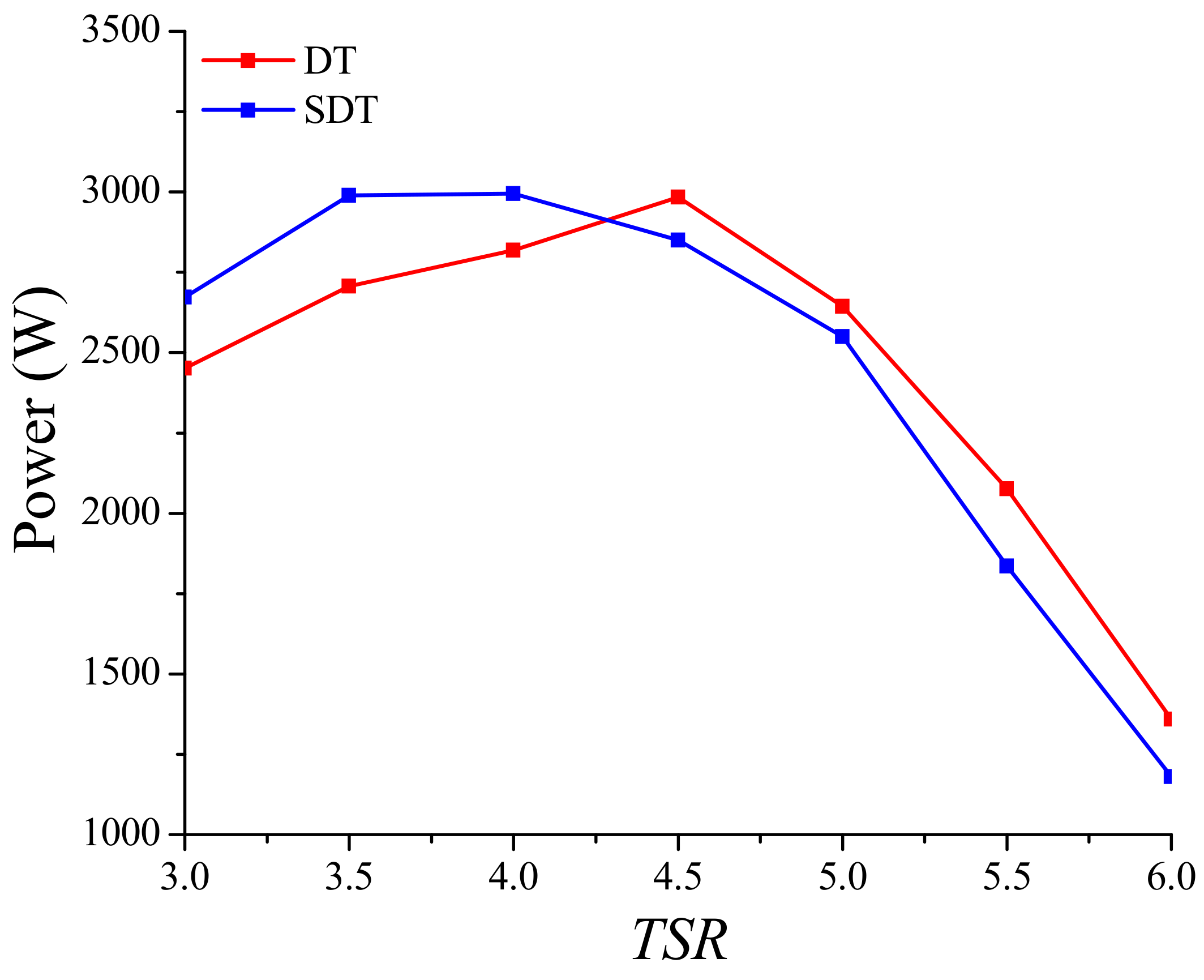
For both cases, calculations are carried out for a free stream velocity of 1.5 m/s and different , which is changed by modifying the rotational speed. The power level comparison between the DT and the SDT is given in Figure 7. The maximum output power of the DT is 2983 W, and the maximum output power of the SDT is 2995 W. The hydrodynamic characteristics comparisons between the DT and the SDT are given in Figure 8, in which the power coefficient, , thrust coefficient, are shown based on the hydrodynamic coefficient definitions, as mentioned before.
It can be observed that the and of each case firstly increase, and reach a maximum, then decrease with the increase of TSR. The structural differences between the DT and the SDT cause the different momentum and load values acting on each blade. For the DT, the optimum at of 4.5 is 0.549, the increases with an increase in when at 3.0 < < 4.5. For the SDT, the optimum at of 4.0 is 0.551, and the increases with an increase in TSR when at 3.0 < < 4.0. The SDT features a higher level when at 3.0 < < 4.25 with respect to the DT, and the range of high performance ( > 0.5) is quite extended (3.1 < < 4.75), which is suitable for operating at lower . In addition, due to the SDT reference area () being considered, the will increase if is based on the swept area, rather than the reference area. In this respect, the swept area is 90% of the reference area, hence increasing of the SDT by a magnitude of 1.2346. On the other hand, the for both cases increase with the increase of when at 3.0 < < 5.0. The SDT has a slightly higher with respect to the DT, obtained at 3.0 < < 4.0, while the DT shows a significant improvement in the at higher . It may also be acknowledged that, since the power generation equipment is integrated into the duct structure as a whole system, and the intermediary supporting structure is removed as mentioned before, the SDT may have lower flow resistance and disturbance than the DT in operating conditions; thus, the stability and reliability of the system is improved. Therefore, the SDT configuration allows the achievement of a higher amount of extracted power at lower , with a potential reduction in flow resistance and disturbance.
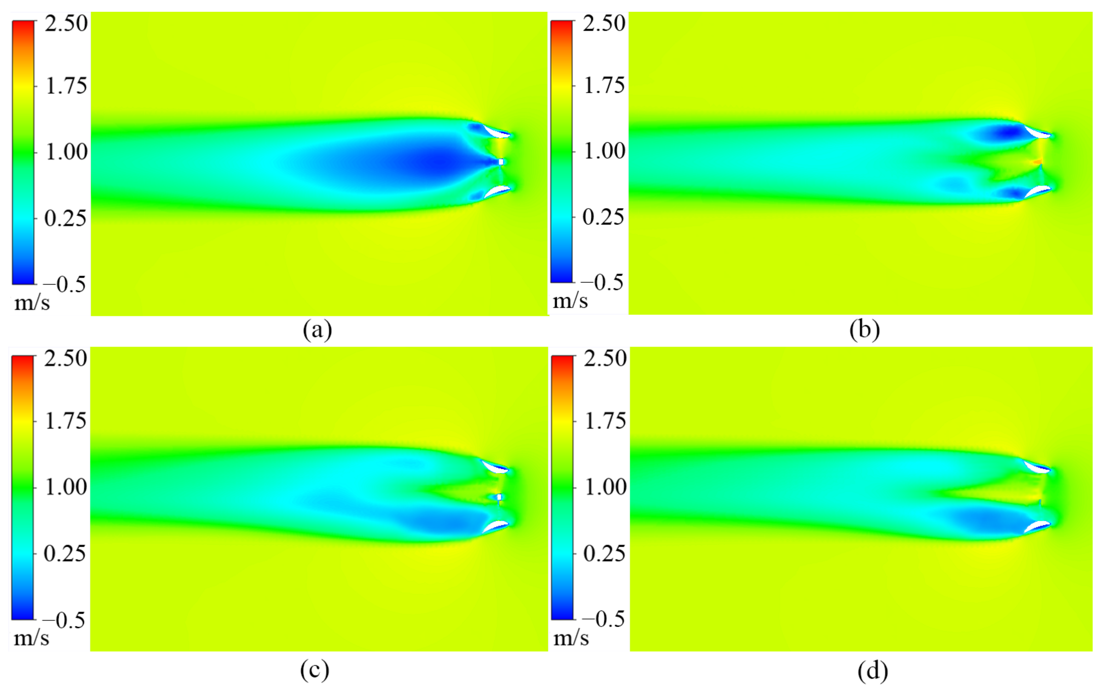
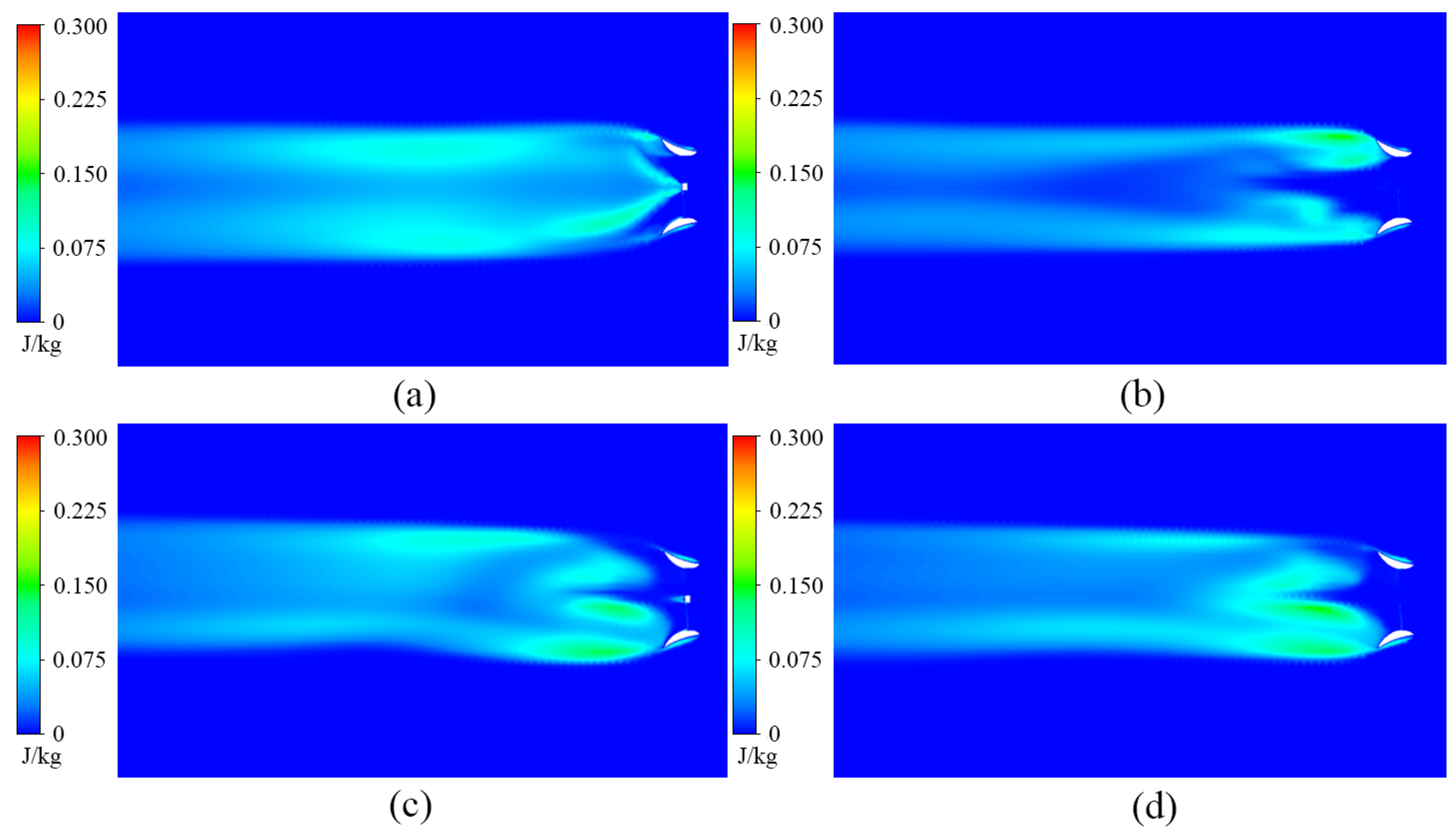
Figure 9 shows the axial velocity distribution comparison between the DT and the SDT at different . It can be observed that the wake shows an obvious low velocity region, with flow separation behind the “trailing edge” of the duct for both cases. Such flow separation phenomenon is extensive at = 4.0, and diminishes at = 6.0 due to the reduction of the velocity gradient between the inner ridge and outer edge of the duct with the increase of . Moreover, for the DT, a part of the incoming flow is blocked by the hub, forming a large range of a low velocity region, which can be clearly identified, as shown in Figure 9a. The velocity distribution varies significantly in accordance to certain regions of the wake, which demonstrates a negative flow structure near hub intermixing at = 4.0, but such a low velocity region is significantly narrowed at = 6.0, as shown in Figure 9c. For the SDT, it shows a larger area interested by the axial velocity increase, as shown in Figure 9b,d. A large mass flow of water is permitted to leak through the open-center structure, forming a high velocity region, which improve the wake structure along the central axis, and such a high velocity region gets bigger with the increase of . Besides the velocity distribution, wakes are also characterized by turbulence levels. Turbulent kinetic energy (TKE) distribution comparison between the DT and the SDT at different is presented in Figure 10. Similarly, as a result of the flow separation, the high TKE is induced behind the trailing edge of the duct for both cases. The wake exhibited a significant degree of TKE induced along the central axis for DT, as shown in Figure 10a,c, where the turbulent flow was shed down the surface, with substantial disorganization within. For the SDT, the highly turbulent flow is not obvious at the central axis area, as shown in Figure 10b,d.
3.2. Energy Loss Characteristics
The entropy production comparison between the DT and the SDT is presented in Figure 11, in which the viscous dissipation entropy production, , turbulent dissipation entropy production, , are shown based on the entropy production definitions as mentioned previously.
It can be observed that, all of the curves have similar shape, but with different values. The velocity gradient between the inner ridge and outer edge of the duct is higher at lower , resulting in flow separation along the duct for both cases, intermixing free-stream velocity and inducing reverse flow at the trailing edge of the duct as discussed previously. Thus, the and the show a high value at lower . With the increase of , the velocity gradient and the flow separation along the duct decrease. However, the blades have a significant momentum exchange effect with the incoming flow at higher , resulting in obvious variations in the velocity profiles around the blades, which lead to large energy loss. Therefore, the and of each case first decreases and then increases with an increase of . In addition, the of each case is much higher than the , which accounts for around 99.8% of the total production at different . Thus, turbulent dissipation is considered the main reason for generating irreversible energy loss for both cases. Moreover, the of the SDT is lessened, compared to that of the DT, with a decrease of 11.3%, as shown in Figure 11a; the of the SDT is also lessened, compared to that of the DT, with a decrease of 6.2%, as shown in Figure 11b. This could be due to the structural differences between the DT and the SDT, as discussed later.
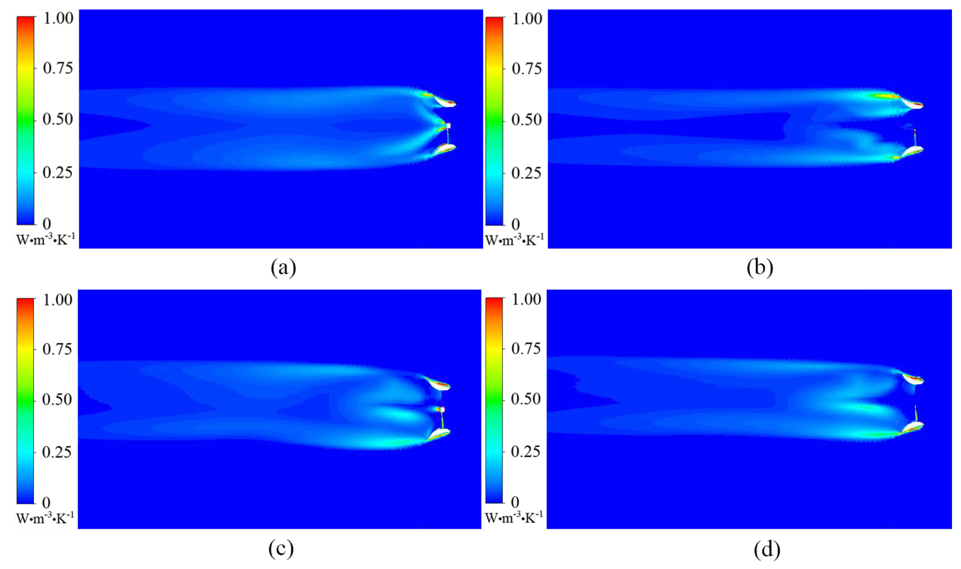
Figure 12 shows the total entropy production rate distribution comparison between the DT and the SDT at different . It can be observed that the entropy production rate behind the trailing edge of the duct is relatively high for both cases, and is extending toward the downstream. This means that the flow separation and the reverse flow induced behind the trailing edge of the duct causes an obvious degree of energy loss as discussed previously. Moreover, from Figure 12a–d, it can be further seen that a higher entropy production rate region appears downstream at = 6.0, compared to that at = 4.0, because the high rotational speed blades strongly interacting with the incoming flow, as discussed previously; thus, the higher causes a higher entropy production. Moreover, the entropy production rate distribution of the SDT is more uniform than that of the DT. As shown in Figure 12a,c, a recognizable entropy production rate region appears behind the hub of the DT, which also matches the low velocity region in Figure 9a,c and the TKE, as shown in Figure 10a,c, behind the hub. However, it is interesting to observe that the above entropy production rate region is not obvious in the SDT shown in Figure 12b,d. The open-center structure has improved the wake structure and avoided the negative flow along the central axis as discussed previously in Figure 9b,d and Figure 10b,d. Therefore, the open-center structure in SDT seems to give an advantageous effect of reducing the entropy production rate region along the central axis, which also explains the entropy production of the SDT is lessened when compared to that of the DT, as shown in Figure 11. In addition, comparing Figure 10 and Figure 12, it can be seen that the TKE distribution is similar to the entropy production rate distribution, in particular, the entropy production analysis has successfully captured the signatures of the energy loss areas induced by flow separation and reverse flow behind the trailing edge of the duct for both cases, and along the central axis for the DT. Therefore, the entropy production analysis used in this study has proven its ability to identify the signatures of energy loss areas due to the flow separation, the reverse flow, and other negative flow factors, weighing how serious the losses are, quantitatively.
4. Conclusions
This work presents a detailed hydrodynamic-energy loss characteristic comparison study for DT and SDT; it was carried out by 3D steady-state computational fluid dynamics simulations and entropy production analysis. From the results, considerable advantages are observed for SDT configuration.
Due to the structural differences between the DT and the SDT and the effect of flow interaction at the upstream surfaces of the blades with that at the downstream blade surfaces, the momentum and load values acting on each blade of both cases are different. The SDT (peak power coefficient of 0.551 at of 4.0) features a higher level when at 3.0 < < 4.25 with respect to the DT (peak power coefficient of 0.549 at of 4.5). The SDT has a slightly higher CT with respect to the DT obtained at 3.0 < < 4.0, while the DT shows a significant improvement in the at higher . Moreover, due to the SDT reference area () being considered, the will increase if is based on the swept area, rather than the reference area. Since the power generation equipment is integrated into the duct structure as a whole system and the intermediary supporting structure is removed, the SDT may have lower flow resistance and disturbance than the DT. In addition, an obvious low velocity region with flow separation is behind the trailing edge of the duct for both cases. As a result of the flow separation, the high TKE is induced at the same area for both cases. The most significant phenomenon, however, is near the central axis—a part of the incoming flow is blocked by the hub of the DT, forming a range of a low velocity region along the central axis. Unlike the DT, the SDT allows a large mass flow of water to leak through the open-center structure, which improves the wake structure along the central axis.
The and the first decrease and then increase with the increase of for both cases. The of each case is much higher than the , which accounts for around 99.8% of the total production at different . Thus, turbulent dissipation is considered the main reason for generating irreversible energy loss. The energy loss is closely related to the negative flow attached on (or shed down) the turbine surface. In particular, turbulent interaction of flow separation, the reverse flow, and other negative flow factors can cause high turbulent entropy generation. Both the and the of the SDT are “lessened” compared to that of the DT at different , also due to the open-center structure, improving the wake structure and avoiding the negative flow along the central axis. The entropy production analysis used in this study has proven its ability to capture the signatures of these energy loss areas, weighing how serious the losses are quantitatively. Moreover, the entropy production analysis can be used as a diagnostic design tool to locate the critical regions for the development and improvement of turbines by using CFD simulations. Accordingly, the insight gained into the structure of the energy loss creates the opportunity to optimize the turbine geometry and better turbine designs can be developed. Further, the entropy production analysis can give deep insight into different flow mechanisms.
Author Contributions
Conceptualization, K.S.; methodology, K.S. and B.Y.; software, B.Y.; validation, K.S.; formal analysis, K.S.; investigation, K.S.; resources, K.S.; data curation, K.S.; writing—original draft preparation, K.S.; writing—review and editing, B.Y.; visualization, B.Y.; supervision, K.S.; project administration, K.S.; funding acquisition, K.S. All authors have read and agreed to the published version of the manuscript.
Funding
This work was supported by the Scientific Research Foundation of Kunming University (grant no. YJL20023).
Institutional Review Board Statement
Not applicable.
Informed Consent Statement
Not applicable.
Data Availability Statement
Not applicable.
Conflicts of Interest
The authors declare no conflict of interest.
References
- Ellabban, O.; Abu-Rub, H.; Blaabjerg, F. Renewable energy resources: Current status, future prospects and their enabling technology. Renew. Sustain. Energy Rev. 2014, 39, 748–764. [Google Scholar] [CrossRef]
- Chen, L.; Li, W.; Li, J.; Fu, Q.; Wang, T. Evolution Trend Research of Global Ocean Power Generation Based on a 45-Year Scientometric Analysis. J. Mar. Sci. Eng. 2021, 9, 218. [Google Scholar] [CrossRef]
- Blunden, L.S.; Bahaj, A.S. Tidal energy resource assessment for tidal stream generators. Proc. Inst. Mech. Eng. Part. A J. Power Energy 2007, 221, 137–146. [Google Scholar] [CrossRef]
- Olczak, A.; Stallard, T.; Feng, T.; Stansby, P.K. Comparison of a rans blade element model for tidal turbine arrays with labor-atory scale measurements of wake velocity and rotor thrust. J. Fluid Struct. 2016, 64, 87–106. [Google Scholar] [CrossRef]
- Ahmed, M.R. Blade sections for wind turbine and tidal current turbine applications-current status and future challenges. Int. J. Energy Res. 2012, 36, 829–844. [Google Scholar] [CrossRef]
- Goundar, J.N.; Ahmed, M.R. Design of a horizontal axis tidal current turbine. Appl. Energy 2013, 111, 161–174. [Google Scholar] [CrossRef]
- Huang, B.; Zhu, G.; Kanemoto, T. Design and performance enhancement of a bi-directional counter-rotating type horizontal axis tidal turbine. Ocean Eng. 2016, 128, 116–123. [Google Scholar] [CrossRef]
- Clarke, J.A.; Connor, G.; Grant, A.D.; Johnstone, C.M. Design and testing of a contra-rotating tidal current turbine. Proc. Inst. Mech. Eng. Part. A J. Power Energy 2007, 221, 171–179. [Google Scholar] [CrossRef] [Green Version]
- Lago, L.; Ponta, F.; Chen, L. Advances and trends in hydrokinetic turbine systems. Energy Sustain. Dev. 2010, 14, 287–296. [Google Scholar] [CrossRef]
- Baratchi, F.; Jeans, T.L.; Gerber, A.G. Assessment of blade element actuator disk method for simulations of ducted tidal turbines. Renew. Energy 2020, 154, 290–304. [Google Scholar] [CrossRef]
- Fleming, C.F.; Willden, R.H. Analysis of bi-directional ducted tidal turbine performance. Int. J. Mar. Energy 2016, 16, 162–173. [Google Scholar] [CrossRef]
- Allsop, S.; Peyrard, C.; Bousseau, P.; Thies, P. Adapting conventional tools to analyse ducted and open centre tidal stream turbines. Int. Mar. Energy J. 2018, 1, 91–99. [Google Scholar] [CrossRef]
- Guo, B.; Wang, D.Z.; Zhou, J.W.; Shi, W.C.; Zhou, X. Performance evaluation of a submerged tidal energy device with a single mooring line. Ocean Eng. 2019, 196, 106791. [Google Scholar] [CrossRef]
- Matheus, M.N.; Rafael, C.F.M.; Taygoara, F.O.; Antonio, C.P.; Brasil, J. An experimental study on the diffuser-enhanced pro-peller hydrokinetic turbines. Renew. Energy 2019, 133, 840–848. [Google Scholar]
- Déborah, A.T.D.; Jerson, R.P.; Paulo, A.S.F. An approach for the optimization of diffuser-augmented hydrokinetic blades free of cavitation. Energy Sustain. Dev. 2018, 45, 142–149. [Google Scholar]
- Rezek, T.J.; Camacho, R.; Filho, N.M.; Limacher, E.J. Design of a Hydrokinetic Turbine Diffuser Based on Optimization and Computational Fluid Dynamics. Appl. Ocean Res. 2020, 107, 102484. [Google Scholar] [CrossRef]
- Tampier, G.; Troncoso, C.; Zilic, F. Numerical analysis of a diffuser-augmented hydrokinetic turbine. Ocean Eng. 2017, 145, 138–147. [Google Scholar] [CrossRef]
- Nachtane, M.; Tarfaoui, M.; Saifaoui, D.; EL Moumen, A.; Hassoon, O.; Benyahia, H. Evaluation of durability of composite materials applied to renewable marine energy: Case of ducted tidal turbine. Energy Rep. 2018, 4, 31–40. [Google Scholar] [CrossRef]
- Borg, M.G.; Xiao, Q.; Allsop, S.; Incecik, A.; Peyrard, C. A numerical performance analysis of a ducted, high-solidity tidal turbine. Renew. Energy 2020, 159, 663–682. [Google Scholar] [CrossRef]
- Open Hydro Ltd. Cape Sharp Tidal, Bay of Fundy, Nova Scotia, Canada. Available online: http://www.openhydro.com/Projects (accessed on 1 March 2018).
- Kock, F.; Herwig, H. Entropy production calculation for turbulent shear flows and their implementation in cfd codes. Int. J. Heat Fluid Flow 2005, 26, 672–680. [Google Scholar] [CrossRef]
- Kock, F.; Herwig, H. Local entropy production in turbulent shear flows: A high-Reynolds number model with wall functions. Int. J. Heat Mass Transf. 2004, 47, 2205–2215. [Google Scholar] [CrossRef]
- Mathieu, J.; Scott, J. An Introduction to Turbulent Flow; Cambridge University Press: Cambridge, UK, 2000. [Google Scholar]
- Menter, F.R. Two-equation eddy-viscosity turbulence models for engineering applications. AIAA J. 1994, 32, 1598–1605. [Google Scholar] [CrossRef] [Green Version]
- Li, D.Y.; Wang, H.J.; Qin, Y.L.; Han, L.; Wei, X.Z.; Qin, D.Q. Entropy production analysis of hysteresis characteristic of a pump-turbine model. Energy Convers. Manag. 2017, 149, 175–191. [Google Scholar] [CrossRef]
- Song, K.; Wang, W.-Q.; Yan, Y. Numerical and experimental analysis of a diffuser-augmented micro-hydro turbine. Ocean Eng. 2018, 171, 590–602. [Google Scholar] [CrossRef]
Figure 1.
Structural comparison between a DT and a SDT: (a) DT; (b) SDT.
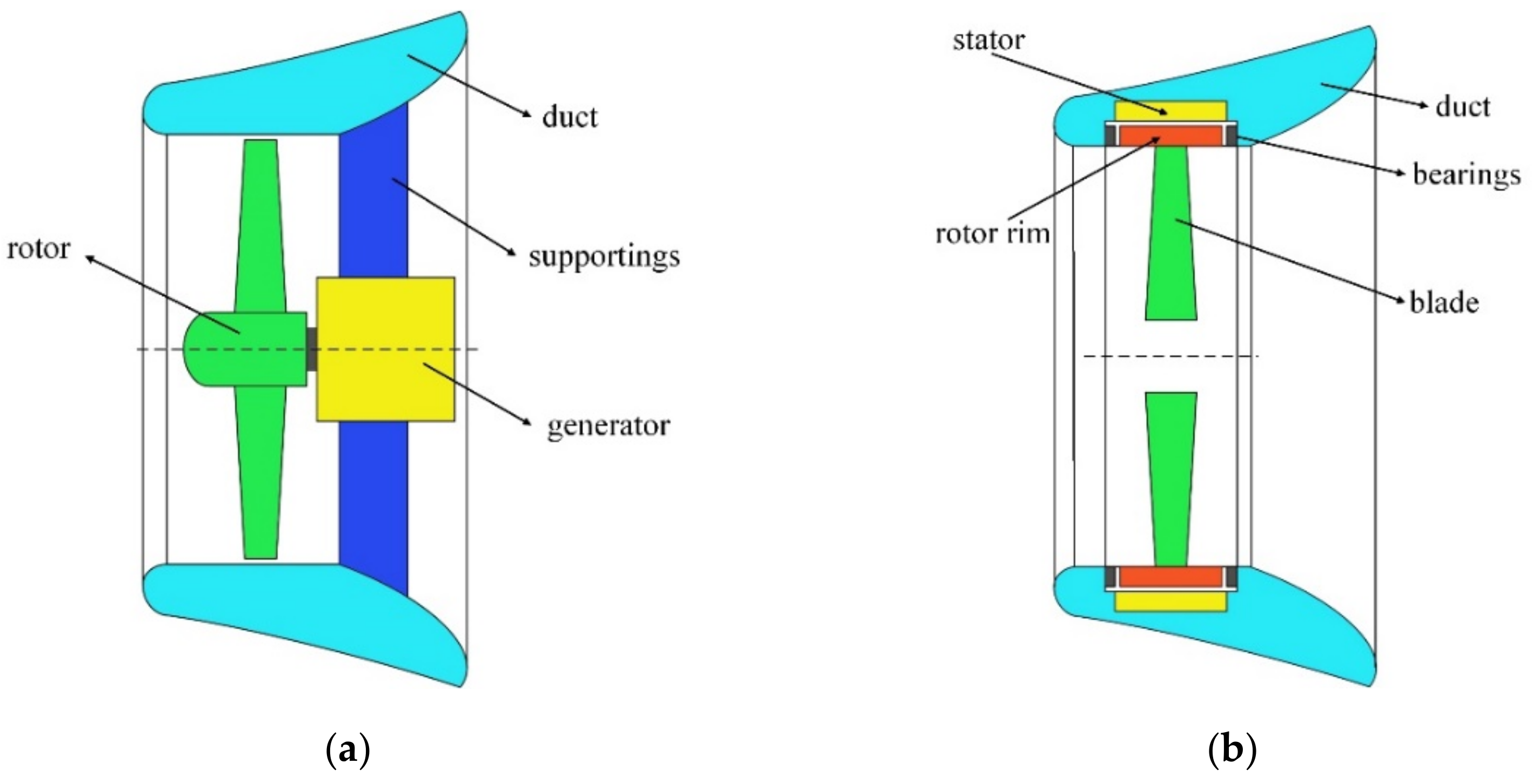
Figure 2.
Dimension diagram of the duct.
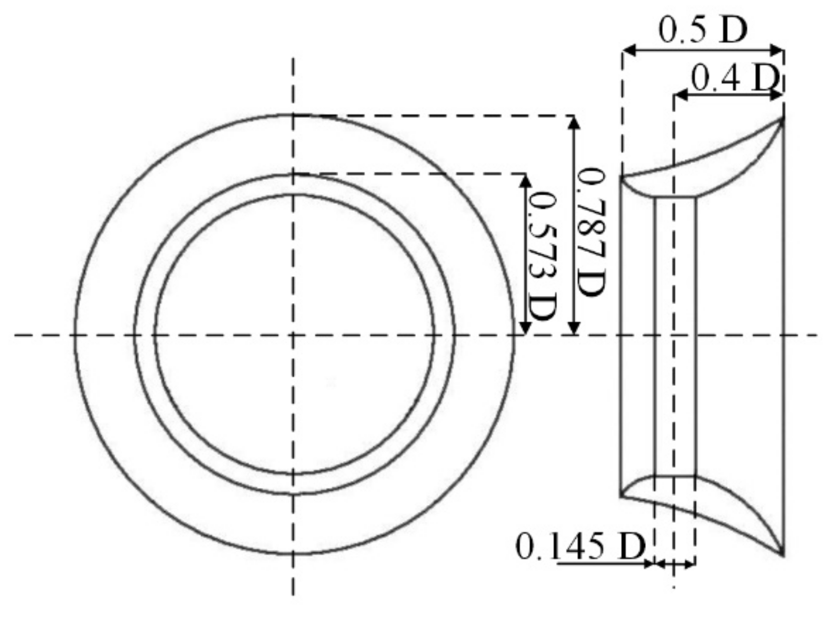
Figure 3.
Schematic view of the DT and the SDT.
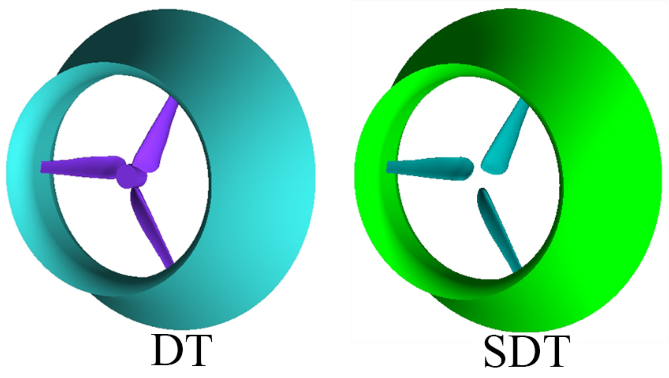
Figure 4.
Calculation domain.
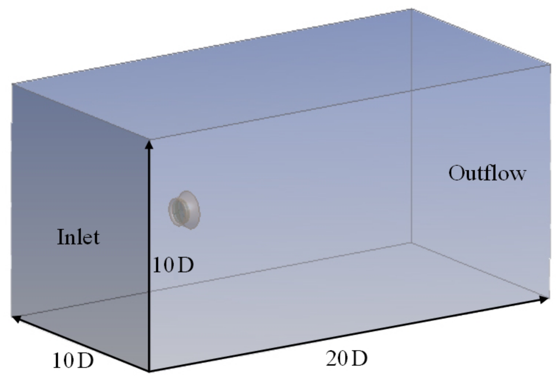
Figure 5.
Mesh distribution: (a) volume mesh; (b) surface mesh.
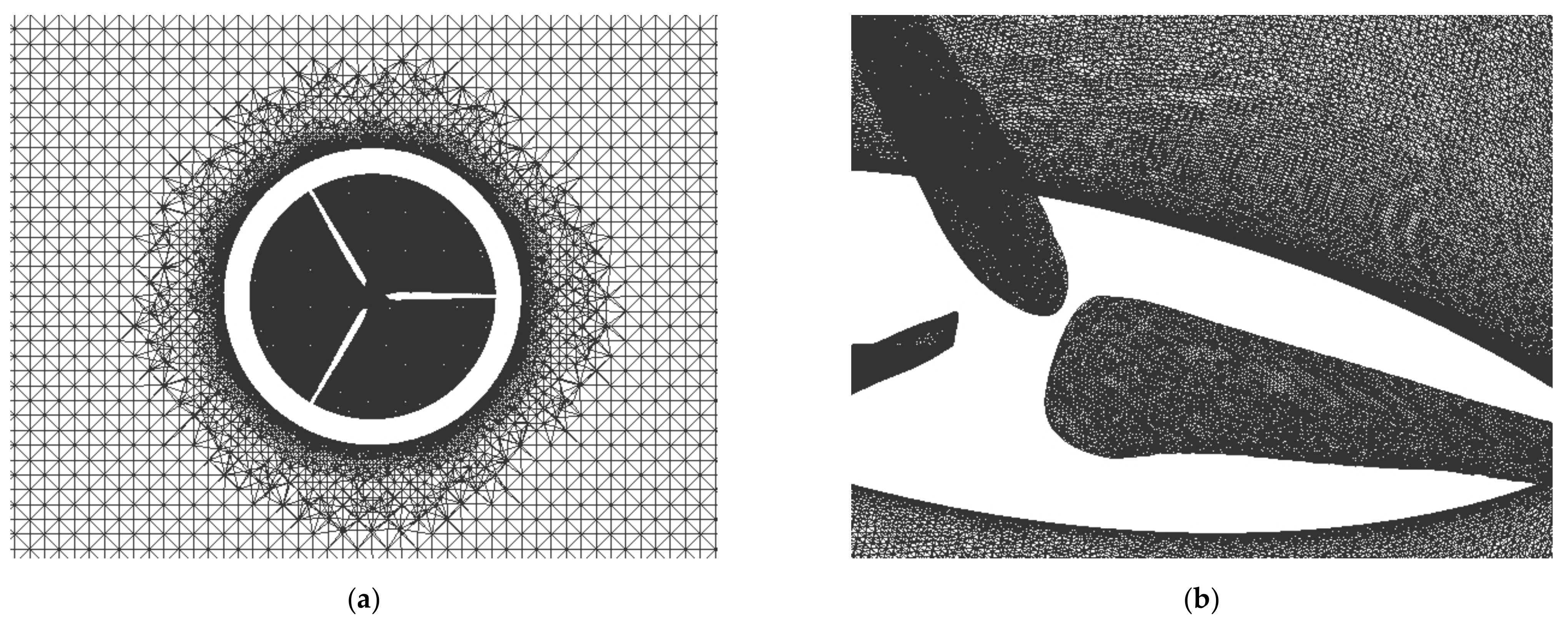
Figure 6.
Validation of the numerical model in this study by the experimental results of Song et al. [26] for the three-blade rotor.
Figure 6.
Validation of the numerical model in this study by the experimental results of Song et al. [26] for the three-blade rotor.
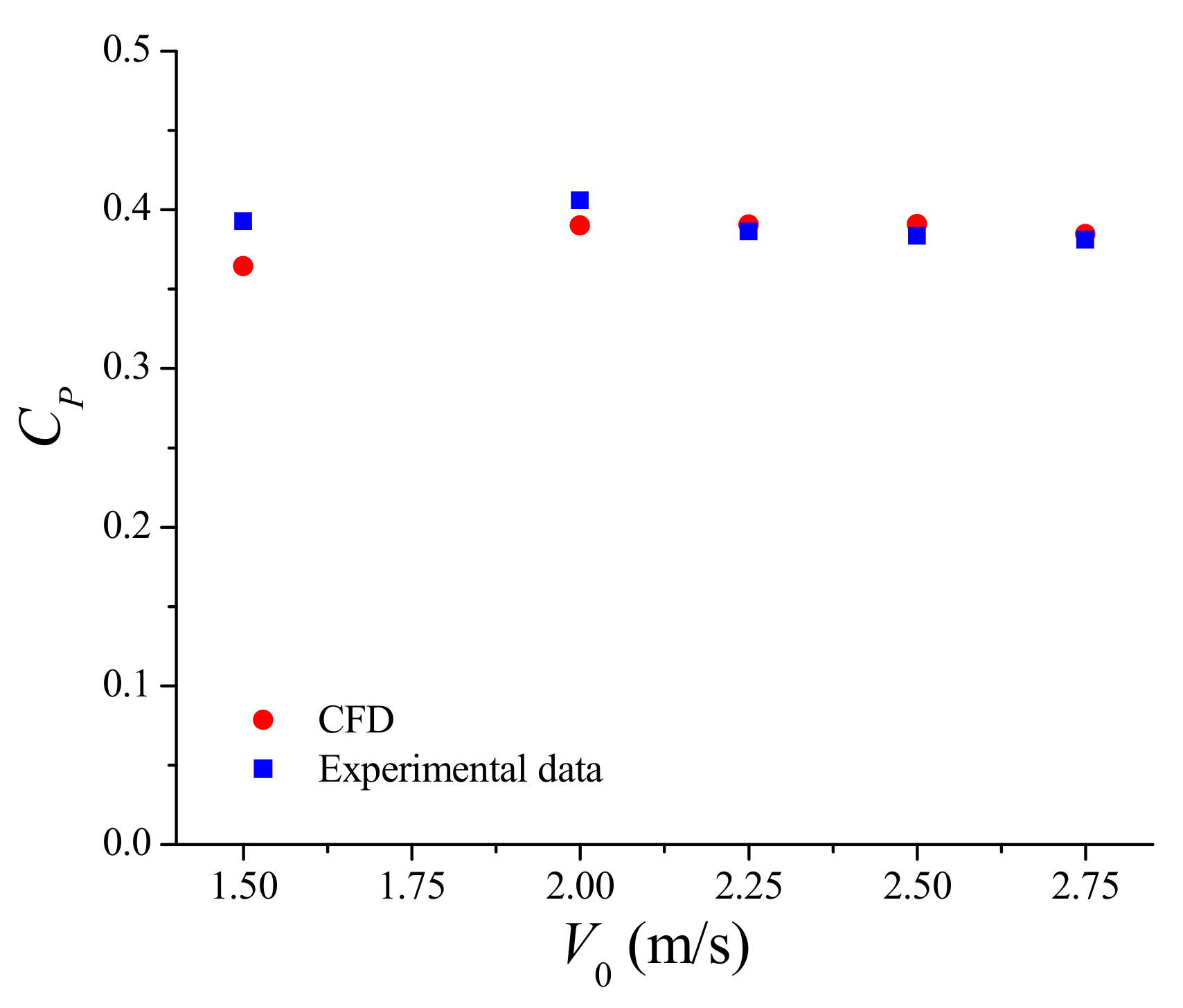
Figure 7.
Power comparison between the DT and the SDT.

Figure 8.
Hydrodynamic characteristic comparisons between the DT and the SDT: (a) power coefficient; (b) thrust coefficient.
Figure 8.
Hydrodynamic characteristic comparisons between the DT and the SDT: (a) power coefficient; (b) thrust coefficient.
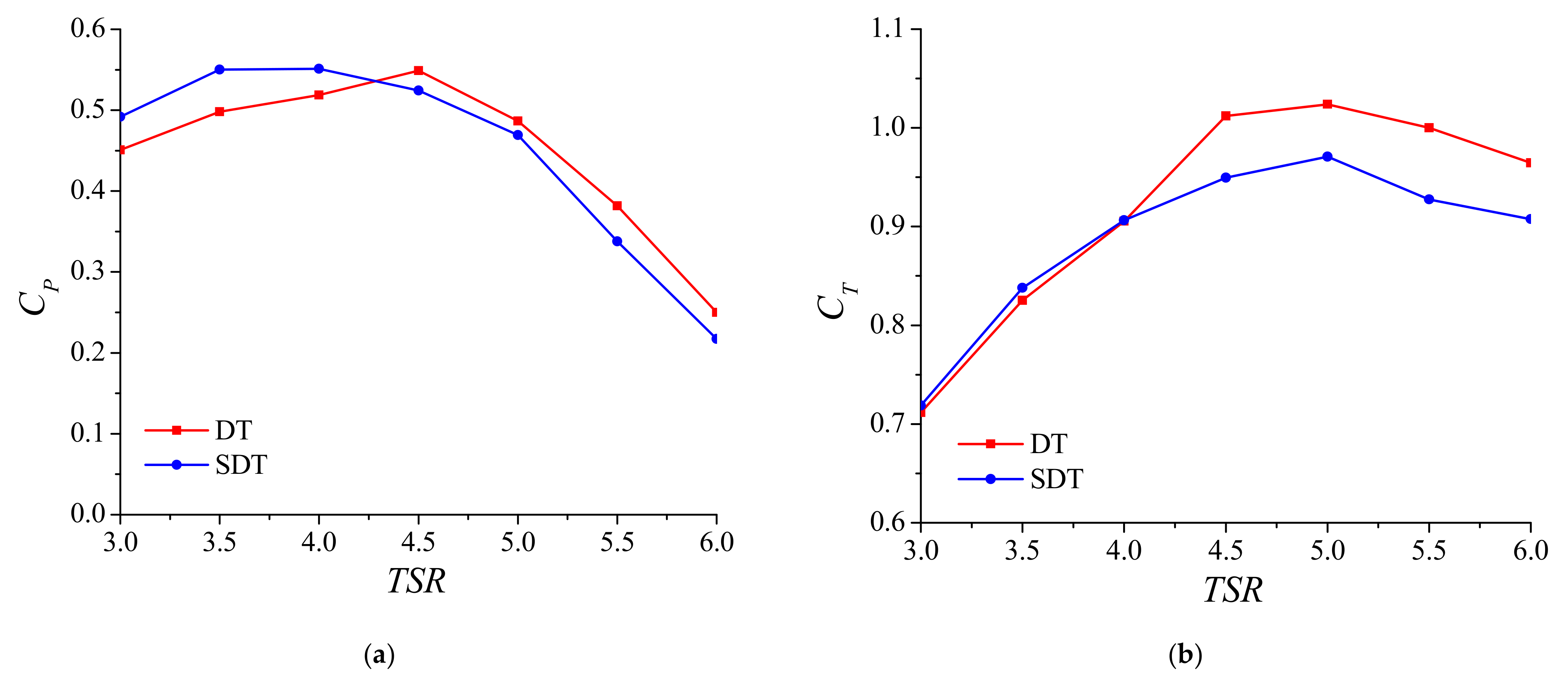
Figure 9.
Axial velocity distribution comparison between the DT and the SDT: (a) DT at = 4.0; (b) SDT at = 4.0; (c) DT at = 6.0; (d) SDT at = 6.0.
Figure 9.
Axial velocity distribution comparison between the DT and the SDT: (a) DT at = 4.0; (b) SDT at = 4.0; (c) DT at = 6.0; (d) SDT at = 6.0.

Figure 10.
Turbulent kinetic energy distribution comparison between the DT and the SDT: (a) DT at = 4.0; (b) SDT at = 4.0; (c) DT at = 6.0; (d) SDT at = 6.0.
Figure 10.
Turbulent kinetic energy distribution comparison between the DT and the SDT: (a) DT at = 4.0; (b) SDT at = 4.0; (c) DT at = 6.0; (d) SDT at = 6.0.

Figure 11.
Entropy production comparison between the DT and the SDT: (a) viscous dissipation entropy production; (b) turbulent dissipation entropy production.
Figure 11.
Entropy production comparison between the DT and the SDT: (a) viscous dissipation entropy production; (b) turbulent dissipation entropy production.
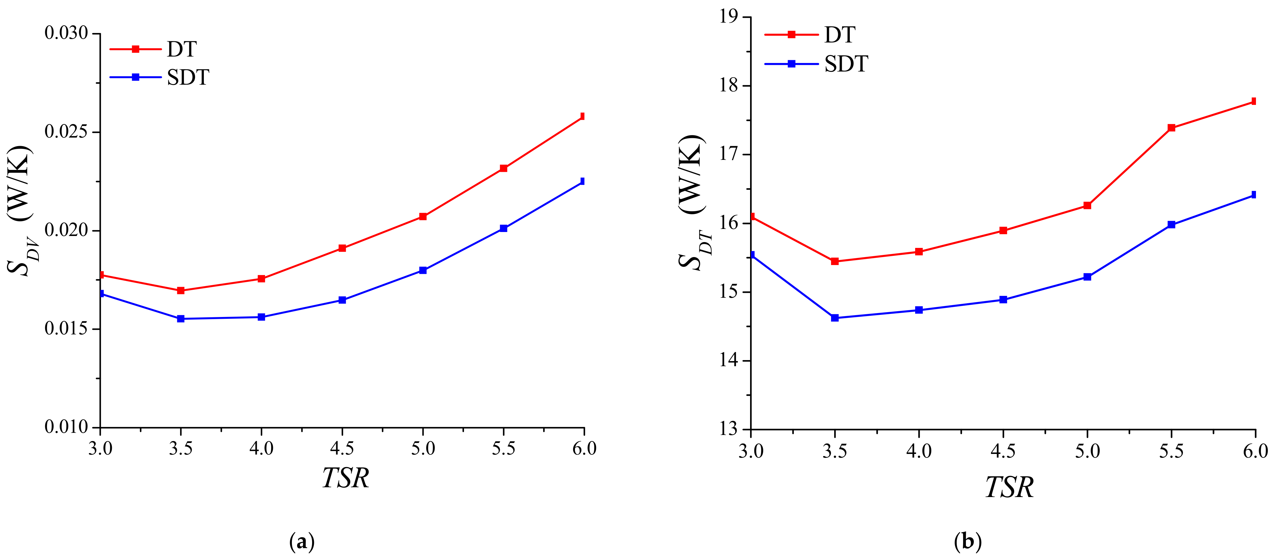
Figure 12.
Total entropy production rate distribution comparison between the DT and the SDT: (a) DT at = 4.0; (b) SDT at = 4.0; (c) DT at = 6.0; (d) SDT at = 6.0.
Figure 12.
Total entropy production rate distribution comparison between the DT and the SDT: (a) DT at = 4.0; (b) SDT at = 4.0; (c) DT at = 6.0; (d) SDT at = 6.0.


Table 1.
Mesh independence assessment.
| Mesh Density | Total Cells (Million) | ||
|---|---|---|---|
| Coarse | 6 | 0.5492 | 0.9046 |
| Medium | 8 | 0.5512 | 0.9063 |
| Fine | 10 | 0.5519 | 0.9068 |
Publisher’s Note: MDPI stays neutral with regard to jurisdictional claims in published maps and institutional affiliations. |
© 2021 by the authors. Licensee MDPI, Basel, Switzerland. This article is an open access article distributed under the terms and conditions of the Creative Commons Attribution (CC BY) license (https://creativecommons.org/licenses/by/4.0/).
Share and Cite
MDPI and ACS Style
Song, K.; Yang, B. A Comparative Study on the Hydrodynamic-Energy Loss Characteristics between a Ducted Turbine and a Shaftless Ducted Turbine. J. Mar. Sci. Eng. 2021, 9, 930. https://doi.org/10.3390/jmse9090930
AMA Style
Song K, Yang B. A Comparative Study on the Hydrodynamic-Energy Loss Characteristics between a Ducted Turbine and a Shaftless Ducted Turbine. Journal of Marine Science and Engineering. 2021; 9(9):930. https://doi.org/10.3390/jmse9090930
Chicago/Turabian StyleSong, Ke, and Bangcheng Yang. 2021. "A Comparative Study on the Hydrodynamic-Energy Loss Characteristics between a Ducted Turbine and a Shaftless Ducted Turbine" Journal of Marine Science and Engineering 9, no. 9: 930. https://doi.org/10.3390/jmse9090930
Note that from the first issue of 2016, this journal uses article numbers instead of page numbers. See further details here.