CICE-LETKF Ensemble Analysis System with Application to Arctic Sea Ice Initialization

Abstract

To study the effectiveness of methods to reduce errors for Arctic Sea ice initialization due to underestimation of background error covariance, an advanced ensemble analysis system has been developed. The system integrates the local ensemble transform Kalman filter (LETKF) with the community ice code (CICE). With a mixed layer ocean model used to compute the sea surface temperature (SST), the experiments on assimilation of observations of sea ice concentration (SIC) have been carried out. Assimilation experiments were performed over a 3-month period from January to March in 1997. The model was sequentially constrained with daily observation data. The effects of observation density, amplification factor for analysis error covariance, and relaxation of disturbance and spread on the results of SIC initialization were studied. It is shown that doubling the density of observation of SIC does not bring significant further improvement on the analysis result; when the ensemble size is doubled, most severe SIC biases in the Labrador, Greenland, Norwegian, and Barents seas are reduced; amplifying the analysis error covariance, relaxing disturbance, and relaxing spread all contribute to improving the reproduction of SIC with amplifying covariance with the largest magnitude.

1. Introduction

Initialization of slow surface processes such as sea ice variation may provide an important contribution to improve climate prediction [1,2]. Accurate initial conditions of sea ice state are vital for numerical sea ice prediction, which is important for human activities such as maritime shipping and oil exploration. In practical applications, observations can be used to optimize sea ice initial conditions through introduction of constraints. Initialization techniques used for improving the quality of initial values have been widely used in atmospheric and oceanic numerical modeling [3].

Sea ice initialization is achieved through assimilation of sea ice observations. Advanced data assimilation (DA) methods combine real observations with model forecasts to improve initial conditions for sea ice prediction [4]. Early studies on sea ice DA are mostly confined to either the statistical optimization method [5,6] or the relaxation technique [7]. Yang et al., (2014) [8] performed experiments on assimilating sea ice thickness into a coupled ice-ocean model using a local singular evolutive interpolated Kalman (SEIK) filter, which is an alternative formulation of an ensemble-based Kalman filter [9]. Toyoda et al., (2016) assimilated sea ice concentrations into a global ocean-sea ice model with the three-dimensional variational (3D-VAR) method [10]. First proposed by Evensen (1994) [11], the ensemble Kalman filter (EnKF) has been a feasible choice for use in operational numerical weather prediction [12]. A coupled ocean-sea ice data assimilation system for the North Atlantic Ocean and Arctic using the ensemble Kalman filter has been run operationally [13]. A series of perfect model observing system simulation experiments (OSSEs) were performed to examine DA algorithms within the EnKF and the relative importance of different observation types [4]. 3D-VAR and EnKF belong to dynamic optimization. Through using model equations, which depict the relationship among model states, as a constraint, dynamic optimization possesses several unique advantages, including a clear physical meaning and greater consistency among the model variables.

Compared to variational algorithms in 3D-VAR or traditional 4D-VAR, EnKF uses time dependent background covariance from the ensemble of forecasts and permits code reuse since it is model independent. Through localization strategy considering observations only within a local patch [14], the local ensemble transform Kalman filter (ETKF [15]) (LETKF) permits small ensemble size and improve the computation efficiency greatly. Like other implementation techniques of EnKF, LETKF is a random-sampling implementation of the Kalman filter (KF), which is written as

$$y_n=H(x_n)+w_n$$

(1)

$$x_{n+1}=M(x_n)+v_n$$

(2)

where subscript n denotes time; $y_n$ is observation; $x_n$ is model state; $w_n$ is error of observation, which obeys a zero mean normal distribution with covariance $R$; $H$ is observation operator; $M$ is model operator; $v_n$ is error of model, which obeys a zero mean normal distribution with covariance $Q$. The KF theory fits for linear system only. In EnKF, $H$ and $M$ are nonlinear.

Houtekamer and Mitchell (1998) applied the EnKF technique to an atmospheric modeling system [16]. Since then, the investigations on the ensemble technique for operational interests have been made extensively (for example, [17]). The computational advantages in high-dimensional EnKF with small ensembles may lead to adverse effects. Since the numerical model is imperfect and the dynamic system is intrinsically nonlinear, the uncertainty of background is inevitably underestimated with a limited ensemble size. The underestimation of error covariance is a common cause of filter divergence. To tackle the problem, many methods have been developed. The often-encountered underestimation of uncertainty can be counteracted with covariance inflation [18]. Through adding a model error term using flow-independent error covariance used in 3D-VAR, Houtekamer et al., (2005) introduced a method known as the “additive covariance inflation” [19]. The random perturbations of known statistics can be added to the analysis or forecast ensemble [20,21]. The “relaxation-to-prior” method, which relaxes the analysis ensemble variance to the forecast ensemble value by mixing background and analysis ensemble perturbations [22] was also introduced. Other measures, such as adding stochastic physics [23,24] and adopting multi-model and/or multi-physical parametrizations [25], were also used.

There have been a few EnKF-based data assimilation systems for sea ice modeling (for example, [4,8,10]) and effects of reducing underestimation of error covariance due to uncertainty of background have been explored. However, there is still uncertainty in effects of factors involved in sea ice data assimilation due to limited work. In the work, an ensemble analysis system for Arctic Sea ice has been developed and systematic investigations on methods reducing error for sea ice initialization due to underestimation of error covariance was performed.

2. Methods and Data

An ensemble analysis system was implemented. Using this system, numerical experiments were set up to study the influences of observation data and methods to reduce underestimation of error covariance on the results of initialization of Arctic Sea ice.

2.1. Ensemble Analysis System

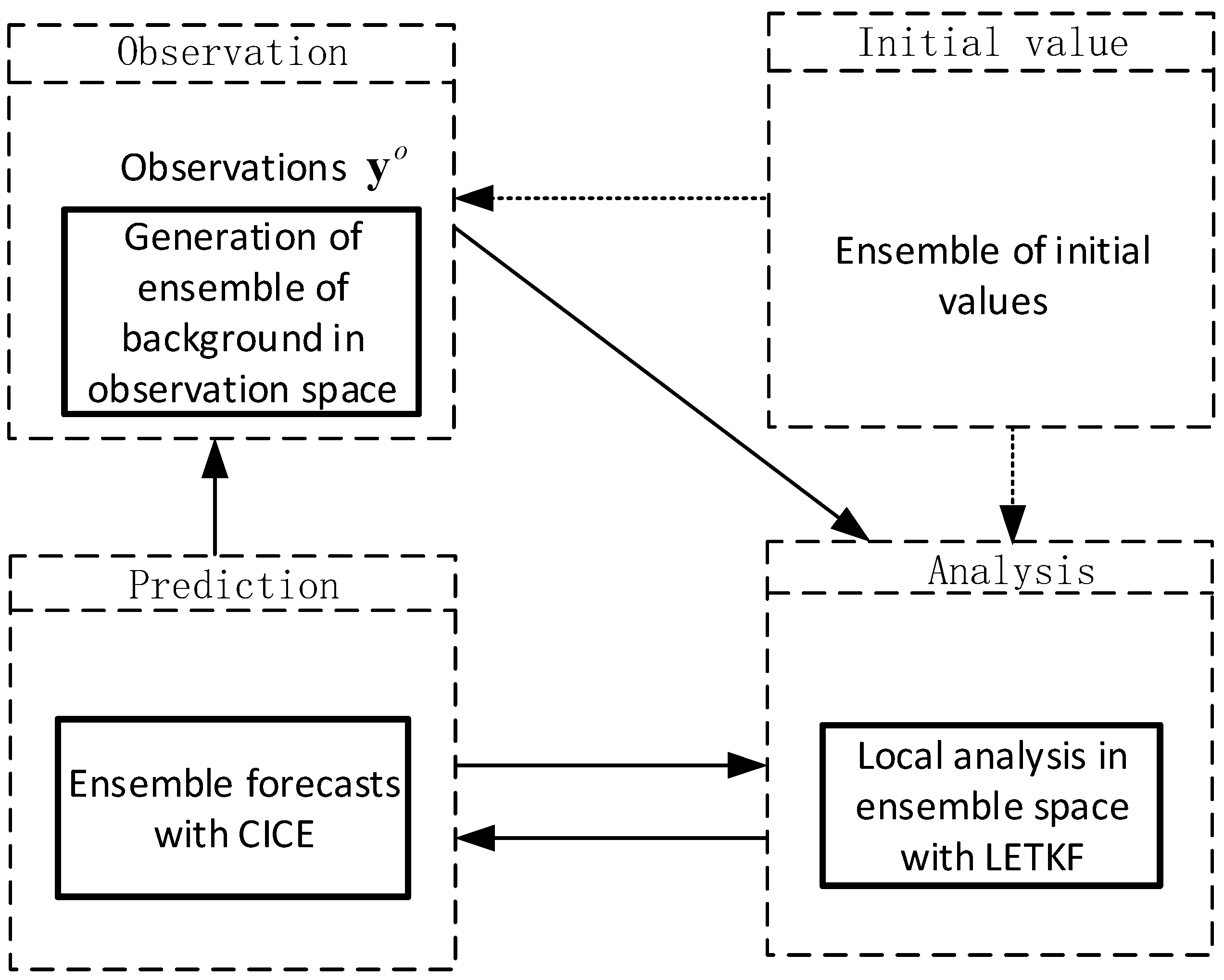
The analysis system integrated the local ensemble transform Kalman filter (LETKF) [14] with the community ice code (CICE) [26] and was named CICE-LETKF. It mainly consisted of three parts: observation, prediction, and analysis (Figure A1). The CICE (version 6.02) was used for ensemble prediction of sea ice evolution in the Arctic. The LETKF was used for local analysis in the ensemble space.

The sea ice model CICE was initially developed by scientists at Los Alamos National Laboratory and has now been the outcome of collaborations with members of the community [26]. CICE mainly consists of three interacting components: ice dynamics, transportation, and physics. The ice dynamics deal the ice pack movement due to forces acting on the sea ice. The transport concerns with advection of sea ice state. The physics, known as Icepack and implemented in CICE as a git submodule, parameterize physical processes which influence the growth and melting of sea ice. The version of the physics package used in the work is 1.1.2. The LETKF is a state-of-the-art approach to data assimilation. It was developed in the University of Maryland [14] and has been constructed as an operational system in numerical weather predictions. The LETKF merges model ensemble solutions and observations to gain optimal model state estimates with improved speed from local processing of each grid point.

Although CICE has been widely used in the community of sea ice modeling, its performance in ensemble analysis system has rarely been seen. Since the LETKF has earned favors in atmospheric DA, its application in sea ice modeling is worth exploring.

2.2. Data

The ERA-interim datasets from the European Center for Medium-Range Weather Forecasts [27] were used as atmospheric forcing fields driving the sea ice model. Downward solar radiation flux, downward long-wave radiation flux, surface air pressure, surface air temperature, surface specific humidity, surface wind, and precipitation rate were used. These variables were in 1.5° × 1.5° longitude-latitude grids. Initial ocean temperature and salinity of the mixed layer ocean model were from World Ocean Atlas 2009 (WOA09) [28,29].

Daily SIC observations from Nimbus-7 SMMR and DMSP SSM/I-SSMIS passive microwave data [30] were used. The data are provided in the polar stereographic projection at a grid cell size of 25 km × 25 km.

3. Theory and Calculation

Theory related to CICE-LETKF analysis was outlined briefly in Section 3.1 and numerical experiments performed were given in Section 3.2.

3.1. Theory

In the prediction part of CICE-LETKF analysis (see Figure A1), ensemble forecasts were performed with

$$x_{n+1,k}^b=M(x_{n,k}^b)$$

(3)

in CICE. Here superscript b implies that the model prediction results are used as background in the observation and analysis parts; k denotes member of the ensemble (k = 1, 2,…, $K$). We define background perturbations in the model space and observation space respectively:

$$X_n^b=[(x_{n,1}^b-{\overline{x}}_n^b),(x_{n,2}^b-{\overline{x}}_n^b),\dots ,(x_{n,K}^b-{\overline{x}}_n^b)]$$

(4)

$$Y_n^b=[(y_{n,1}^b-{\overline{y}}_n^b),(y_{n,2}^b-{\overline{y}}_n^b),\dots ,(y_{n,K}^b-{\overline{y}}_n^b)]$$

(5)

where the overbar represents the ensemble average; $y_{n,k}^b$ is the background in observation space and is computed in the observation part (Figure A1) with equation

$$y_{n,k}^b=H(x_{n,k}^b)$$

(6)

The analysis determines the linear combination of ensemble solutions (from Equation (3)) that best fits the observations $y^o$. The LETKF assimilates all observations simultaneously and acquires its speed from local processing of each grid point. In LETKF, the entire grid is separated into local patches (one patch is a local region centered around an analysis grid point) and analysis is performed for each local patch. In the analysis part, the following computations are performed:

$${\overline{x}}_{n(l)}^a={\overline{x}}_{n(l)}^b+X_{n(l)}^b{\overline{w}}_{n(l)}$$

(7)

$$X_{n(l)}^a=X_{n(l)}^b{[(K-1){\tilde{P}}_{n(l)}^a]}^{1/2}$$

(8)

where the subscript (l) denotes local patch; ${\overline{w}}_{n(l)}$ is a weighting vector connected with observational increment; ${\tilde{P}}_{n(l)}^a$ is the analysis error covariance in the ensemble space; $X_{n(l)}^a$ is analysis perturbations in a local patch, i.e.,

$$X_{n(l)}^a=[(x_{n,1(l)}^a-{\overline{x}}_{n(l)}^a),(x_{n,2(l)}^a-{\overline{x}}_{n(l)}^a),\dots ,(x_{n,K(l)}^a-{\overline{x}}_{n(l)}^a)]$$

(9)

${\overline{w}}_{n(l)}$ is computed by

$${\overline{w}}_{n(l)}={\tilde{P}}_{n(l)}^a{(Y_{n(l)}^b)}^T{R}_{(l)}^{-1}(y_{n(l)}^o-{\overline{y}}_{n(l)}^b)$$

(10)

and ${\tilde{P}}_{n(l)}^a$ is computed by

$${\tilde{P}}_{n(l)}^a={[{(Y_{n(l)}^b)}^T{R}_{(l)}^{-1}(Y_{(l)}^b)+(K-1)I]}^{-1}$$

(11)

The LETKF is a transform square root filter. The analysis ensemble is explicitly expressed as a linear combination of the forecast ensemble. The global analysis ensemble $x_{n,k}^a$ (k = 1,…, $K$) is obtained by gathering the values for ${\overline{x}}_{n(l)}^a$ and $X_{n(l)}^a$ at all the analysis grid points. More details on the LETKF algorithm and its implementation can be found in [14].

3.2. Calculation

In the numerical experiments with CICE-LETKF, grids in a coordinate system on the stereographic projection plane were used. The analysis was performed at the time of observation (i.e., 3D analysis). The center of the simulation domain is the North Pole. The model has a horizontal resolution of 50 km, with a time step of 3600 s for thermodynamics. In the projection, the standard longitude is 0° E, and the true latitude is 60° N. With a grid size of 50 km and an extent covering the Ice Island and Bering Strait, 160 grids in the x direction and 100 grids in the y direction are used.

Four groups of numerical experiments (G1–G4), which dealt with the use of observation, size of ensembles, initial values for prediction model, and parameters of analysis system respectively, were designed (

Table 1. Experiments in group G1.

Name	Description
OBSC	Ensemble size was 20; the initial values for the ensemble prediction were randomly taken from the restart field of control run without DA every 7 days; no observation was assimilated in the ensemble simulation.
OBS1	Same as OBSC except the SIC adopted every 4 grids from the observation field was assimilated.
OBS2	Same as OBSC except the SIC adopted every 2 grids from the observation field was assimilated.

,

Table 2. Experiments in group G2.

Name	Description
ENSC	Ensemble size was 20; the initial values for the ensemble prediction were randomly taken from the restart field of control run without DA every 3 days; the SIC was adopted every 4 grids from the observation field.
ENS1	Same as ENSC except that ensemble size was 40.

,

Table 3. Experiments in group G3.

Name	Description
INIC	Ensemble size was 20; the initial values for the ensemble prediction were randomly taken from the restart field of control run without DA every 7 days; the SIC was adopted every 4 grids from the observation field. It was identical to OBS1 in Table 1.
INI1	Same as INIC except that the initial values for the ensemble prediction were randomly taken from the restart field of control run without DA every 3 days. It was identical to ENSC in Table 2.

and

Table 4. Experiments in group G4.

Name	Description
PARC	Ensemble size was 20; the initial values for the ensemble prediction were randomly taken from the restart field of control run without DA every 7 days; the SIC adopted every 4 grids from the observation field was assimilated. It was identical to OBS1 in Table 1.
PAR1	Same as PARC except that covariance inflation was performed in the filtering with $\rho$ = 2 in Equation (12).
PAR2	Same as PARC except that perturbation relaxation was performed in the filtering with $\beta$ = 0.5 in Equation (13).
PAR3	Same as PARC except that spread relaxation was performed in the filtering with $\gamma$ = 0.5 in Equation (14).

). In G1, the influence of assimilation of observation variable (compare OBS1 to OBSC) as well SIC density (compare OBS2 to OBS1) was studied. The initial ensemble is generated from samples at specific intervals in time of a control run without DA; these samples are assumed to reflect the statistical properties of the sampling space of sea ice initial conditions. Shorter intervals mean smaller spread, longer intervals mean larger spread. In G2, the influence of ensemble size (compare ENS1 to ENSC) was investigated. In G3, the influences of initial values (compare INI1 to INIC) were examined. The method to generate sea ice initial value ensemble was borrowed from work of atmospheric modeling [12]. The choice of interval for selection of member for initial value from restarts of control run without DA is presumed to reflect the statistical property of sampling space for sea ice initial values. In G4, covariance inflation parameter (i.e., $\rho$ in Equation (12), compare Equation (12) to Equation (11)), perturbation relaxation (Equation (13)), and spread relaxation (Equation (14)) were introduced in the filtering and their effects (compare PAR1 to PARC, PAR2 to PARC, and PAR3 to PARC) were studied. To alleviate the underestimation of uncertainties of background fields, the covariance was inflated by modifying the computation of the analysis error covariance in Equation (11):

$${\tilde{P}}_{n(l)}^a={[{(Y_{n(l)}^b)}^T{R}_{(l)}^{-1}(Y_{(l)}^b)+(K-1)I/\rho ]}^{-1}$$

(12)

here $\rho$ was the inflation parameter. To counteract the underestimation of uncertainty, relaxations in the perturbation and the spread were introduced:

$$X_{n(l)}^a=(1-\beta )X_{n(l)}^a+\beta X_{n(l)}^b$$

(13)

$$X_{n(l)}^a=(1+\gamma \frac{s^b-s^a}{s^a})X_{n(l)}^a$$

(14)

where $\beta$ and $\gamma$ were coefficients for the perturbation relaxation and spread relaxation respectively; $\mathbf{s}$ was the spread.

In the analysis with CICE-LETKF, if it occurred that the SIC was negative, the SIC was set to zero. The next cycle was restarted from the analysis results directly. In all experiments, the initial ensemble members were chosen from predictions of the control run without DA, which was generated by running CICE for 1 year from restart of a 20-year integration. The starting time of the control run without DA was set to 0000 UTC on 1 January 1997. Ensemble analysis was performed for the period ranging from 1 January 1997 to 1 April 1997.

4. Results and Discussion

Sea ice area fraction (SIAF) from the analysis experiments has been analyzed. The spatial distribution of SIAF averaged from January to March in 1997 for the satellite observation is given in Figure 1a. It is shown that ice extent during winter in the Arctic Ocean is largely constrained by the surrounding land masses with the open space for ice cover extension in the Greenland, Norwegian, and Barents seas. Significant SIAF variations exist mainly in the Labrador, Greenland, Norwegian, and Barents seas in the winter. With no observation data assimilated (the experiment OBSC in Table 1), the ensemble simulation produces too much sea ice in the Labrador and Barents seas. There is too much sea ice in the Greenland Sea off the eastern Greenland coast and to little SIAF in the Greenland Sea adjacent to the southern Greenland (Figure 1b). The differences in SIAF between OBSC and observation are mostly less than 0.2 in the Arctic Ocean. When the observed SIC is assimilated (experiments OBS1 and OBS2 in Table 1), the discrepancies between the results from analysis and those from the observation are reduced (compare Figure 1c,d to Figure 1b). It should be noted that since Figure 1b–d present differences between two results, to obtain the difference between OBS1/OBS2 and observation, results of Figure 1c,d and Figure 1a should be added. The signs of values in Figure 1c,d are almost opposite to those in Figure 1a everywhere. This means that the biases in reproduced SIAF are decreased through assimilating observed SIC. The improvement is evident in the entire domain, especially in the Labrador, Greenland, Norwegian, and Barents seas where seasonal variation of sea ice is large. The differences between OBS1 and OBS2 is small (compare Figure 1c to Figure 1d), implying that the density of observation data does not have great impact on the analysis results.

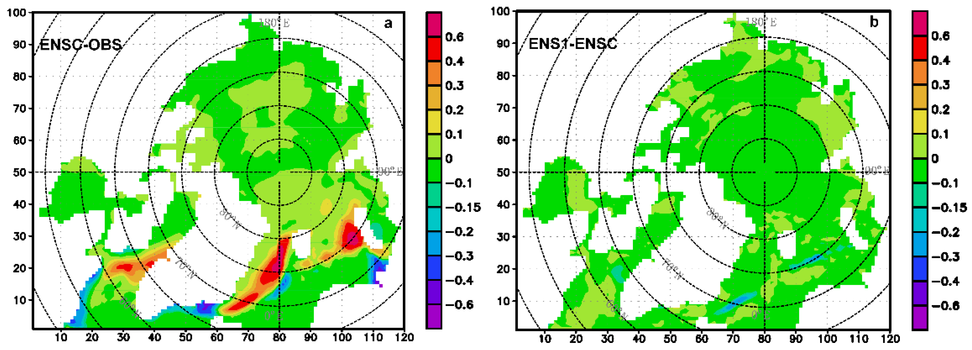
When the ensemble size is doubled (experiment ENS1 in Table 2), most severe SIAF biases in the Labrador, Greenland, Norwegian, and Barents seas are reduced (see Figure 2). As an ensemble analysis system, CICE-LETKF produces the analysis ensemble with the improved mean and perturbations sampling the covariance of analysis error through modifying the ensemble of forecast. Therefore, larger ensembles provide a better estimate of the underlying distribution and contribute to the improvement of analysis results. However, bigger ensemble size means larger burden of computation. It is shown that the magnitude of improvement is relatively small compared to those of experiments assimilating observations (compare Figure 2b to Figure 1c,d).

At the beginning of ensemble analysis, CICE-LETKF starts from the ensemble of initial values, which is used to generate ensemble of background in observation space in the observation step and used as background field in model space in the analysis step (Figure A1). After that, the loop cycle of analysis-prediction-observation starts. In CICE-LETKF, the information of initially sampled covariance of background error propagates and influences the later analysis results through analysis-prediction-observation cycle. Compared to results from INIC in Table 3, the produced biases in the northern Labrador, eastern Greenland and northeastern Barents seas are enlarged in INI1 (see Figure 3). This is due to the smaller perturbation of initial values in INI1 than that in INIC. The larger spread in INIC leads to larger spread in simulation result (background field), which contributes to the reduction of bias.

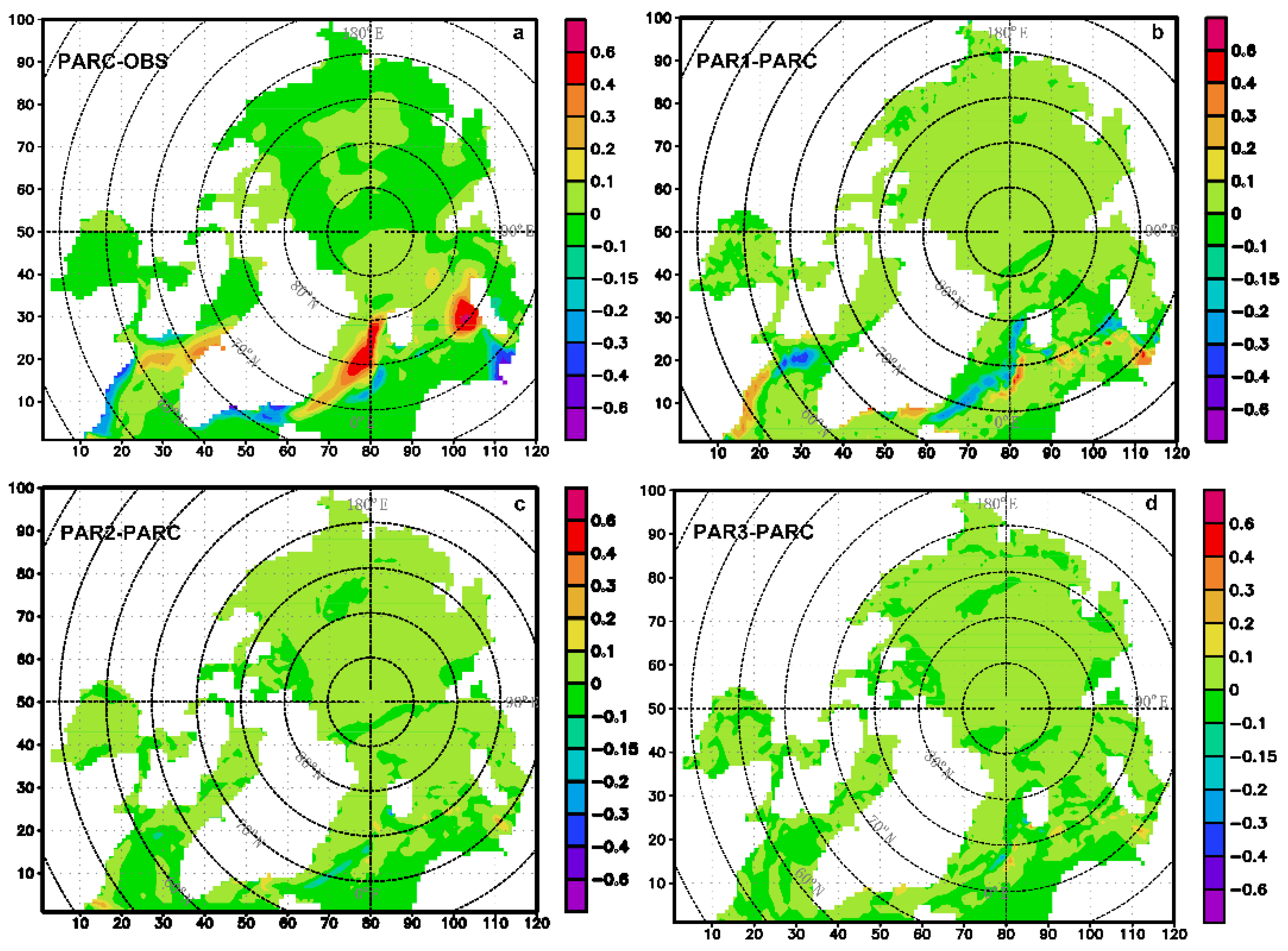
The introduction of covariance inflation parameter ($\rho$ = 2 is used in Equation (12)) (experiment PAR1 in Table 4) significantly improve the analysis results in mean SIAF (see Figure 4a,b). In regions with large biases of SIAF as the western Labrador Sea near the coast, northern Labrador Sea, southern Greenland Sea near the coast, eastern Greenland Sea, northeastern Barents Sea and southeastern Barents Sea near the coast, the analysis errors are reduced greatly. For the linear observation operator used here, the introduction of covariance inflation parameter is equivalent to using an inflation factor of $\sqrt{2}$ in ensemble perturbations [24]. Perturbation relaxation (experiment PAR2 in Table 4) and spread relaxation (experiment PAR1 in Table 4) also improve the analysis results (see Figure 4a,c,d), whereas the magnitude of improvement is smaller than that of covariance inflation (compare Figure 4c,d to Figure 4b). The magnitude of improvement in PAR2 is comparable to that in PAR3 (compare Figure 4c to Figure 4d).

In the experiments, the inflation parameter is constant. In practical application, observation coverage may vary in space and time. In such cases, the inflation parameter can be made a function of time and position. Moreover, the impact of local patch size on SIC analysis also need to be studied.

Through integrating another version of CICE (CICE5) with the ensemble adjustment Kalman filter (EAKF) in the Data Assimilation Research Testbed (DART), Zhang et al., (2018) performed experiments assimilating sea ice thickness (SIT) using perfect model OSSEs regarding the shortage of SIT observation [4]. Their study show that largest simulation improvements are produced when SIT and SIC are jointly assimilated. From work by Yang et al., (2014) using a local SEIK filter, it is also found that the SIC forecasts agree better with observations when satellite observation of SIT is assimilated [8]. Study the effects of assimilation of other observations such as sea ice velocity and SIT in the context of CICE-LETKF is necessary.

From studies on the role of atmospheric uncertainty for the assimilation and prediction of Arctic Sea ice, it is shown that sea ice assimilation is sensitive to atmospheric uncertainty and the model data misfit improves when atmospheric uncertainty is considered [31,32]. In the experiments, atmospheric forcing is identical and the uncertainty in the forcing fields are not considered. Since atmospheric forcing is a large determining factor in sea ice modeling, effects of atmospheric uncertainty in CICE-LETKF framework deserve study in later work.

The CICE-LETKF is a novel ensemble analysis system. It is fast due to the high parallel computation efficiency of its components, CICE and LETKF. Some important work such as the role of atmospheric uncertainty and the effects of other observations (for example, sea ice velocity and SIT) can be explored with the CICE-LETKF system.

5. Conclusions

A CICE-LETKF analysis system has been implemented and sensitivity experiments on SIC analysis have been made. Results from the experiments show that assimilating SIC observation can improve the result of SIC initialization significantly; the density of observation data, number of ensembles, perturbations of initial value and relaxations regarding to the uncertainties of background fields contribute to the results; the inflation of covariance has the greatest influence on the performance of the analysis system.

References

1. Liu, X.Y.; Liu, H.L.; Li, W.; Zhang, X.H.; Yu, R.C.; Yu, Y.Q. Numerical simulation of atmosphere-ocean-sea ice interaction during the interannual cycle in high northern latitudes. Acta Meteorol. Sin. 2008, 22, 119–128. [Google Scholar]
2. Shepherd, T.G.; Arblaster, J.M.; Bitz, C.M.; Furevik, T.; Goosse, H.; Kattsov, V.M.; Marshall, J.; Ryabinin, V.; Walsh, J.E. Report on WCRP workshop on seasonal to multi-decadal predictability of polar climate. SPARC Newsl. 2011, 36, 11–19. [Google Scholar]
3. Liu, X.; Zhang, L. Study on optimization of sea ice concentration with adjoint method. J. Coast. Res. 2018, 84, 44–50. [Google Scholar] [CrossRef]
4. Zhang, Y.F.; Bitz, C.M.; Anderson, J.L.; Collins, N.; Hendricks, J.; Hoar, T.; Raeder, K.; Massonnet, F. Insights on sea ice data assimilation from perfect model observing system simulation experiments. J. Clim. 2018, 31, 5911–5926. [Google Scholar] [CrossRef]
5. Meier, W.N.; Maslanik, J.A.; Fowler, C.W. Error analysis and assimilation of remotely sensed ice motion within an Arctic sea ice model. J. Geophys. Res. 2000, 105, 3339–3356. [Google Scholar] [CrossRef]
6. Zhang, J.; Thomas, D.R.; Rothrock, D.A.; Lindsay, R.W.; Yu, Y.; Kwok, R. Assimilation of ice motion observations and comparisons with submarine ice thickness data. J. Geophys. Res. 2003, 108, 3170. [Google Scholar] [CrossRef] [Green Version]
7. Tietsche, S.; Notz, D.; Jungclaus, J.H.; Marotzke, J. Assimilation of sea-ice concentration in a global climate model—Physical and statistical aspects. Ocean Sci. 2013, 92, 19–36. [Google Scholar] [CrossRef] [Green Version]
8. Yang, Q.; Losa, S.N.; Losch, M.; Tian-Kunze, X.; Nerger, L.; Liu, J.; Kaleschke, L.; Zhang, Z. Assimilating SMOS sea ice thickness into a coupled ice-ocean model using a local SEIK filter. J. Geophys. Res. Oceans 2014, 119, 6680–6692. [Google Scholar] [CrossRef] [Green Version]
9. Nerger, L.; Danilov, S.; Hiller, W.; Schröter, J. Using sea-level data to constrain a finite-element primitive-equation ocean model with a local SEIK filter. Ocean Dyn. 2006, 56, 634–649. [Google Scholar] [CrossRef] [Green Version]
10. Toyoda, T.; Fujii, Y.; Yasuda, T.; Usui, N.; Ogawa, K.; Kuragano, T.; Tsujino, H.; Kamachi, M. Data assimilation of sea ice concentration into a global ocean—Sea ice model with corrections for atmospheric forcing and ocean temperature fields. J. Oceanogr. 2016, 72, 235–262. [Google Scholar] [CrossRef]
11. Evensen, G. Sequential data assimilation with a nonlinear quasigeostrophic model using Monte-Carlo methods to forecast error statistics. J. Geophys. Res. 1994, 99, 10143–10162. [Google Scholar] [CrossRef]
12. Miyoshi, T.; Yamane, S. Local ensemble transform Kalman filtering with an AGCM at a T159/L48 resolution. Mon. Weather Rev. 2007, 135, 3841–3861. [Google Scholar] [CrossRef] [Green Version]
13. Sakov, P.; Counillon, F.; Bertino, L.; Lisæter, K.A.; Oke, P.R.; Korablev, A. TOPAZ4: An ocean-sea ice data assimilation system for the North Atlantic and Arctic. Ocean Sci. 2012, 8, 633–656. [Google Scholar] [CrossRef] [Green Version]
14. Hunt, B.R.; Kostelich, E.J.; Szunyogh, I. Efficient data assimilation for spatiotemporal chaos: A local ensemble trans-form Kalman filter. Phys. D 2007, 230, 112–126. [Google Scholar] [CrossRef] [Green Version]
15. Bishop, C.H.; Etherton, B.; Majumdar, S.J. Adaptive sampling with the ensemble transform Kalman fifilter part I: The theoretical aspects. Mon. Weather Rev. 2001, 129, 420–436. [Google Scholar] [CrossRef]
16. Houtekamer, P.L.; Mitchell, H.L. Data assimilation using an ensemble Kalman filter technique. Mon. Weather Rev. 1998, 126, 796–811. [Google Scholar] [CrossRef]
17. Shin, S.; Kang, J.S.; Jo, Y. The Local Ensemble Transform Kalman Filter (LETKF) with a Global NWP Model on the Cubed Sphere. Pure Appl. Geophys. 2016, 173, 2555–2570. [Google Scholar] [CrossRef] [Green Version]
18. Anderson, J.L.; Anderson, S.L. A Monte Carlo implementation of the nonlinear filtering problem to produce ensemble assimilations and forecasts. Mon. Weather Rev. 1999, 127, 2741–2758. [Google Scholar] [CrossRef]
19. Houtekamer, P.L.; Mitchell, H.L.; Pellerin, G.; Buehner, M.; Charron, M.; Spacek, L.; Hansen, B. Atmospheric Data Assimilation with an Ensemble Kalman Filter: Results with Real Observations. Mon. Weather Rev. 2005, 133, 604–620. [Google Scholar] [CrossRef] [Green Version]
20. Hamill, T.M.; Whitaker, J.S. Accounting for the error due to unresolved scales in ensemble data assimilation: A comparison of different approaches. Mon. Weather Rev. 2005, 133, 3132–3147. [Google Scholar] [CrossRef]
21. Whitaker, J.S.; Hamill, T.M.; Wei, X.; Song, Y.; Toth, Z. Ensemble data assimilation with the NCEP global forecast system. Mon. Weather Rev. 2008, 136, 463–482. [Google Scholar] [CrossRef] [Green Version]
22. Zhang, F.; Snyder, C.; Sun, J. Impacts of initial estimate and observation availability on convective-scale data assimilation with an ensemble Kalman filter. Mon. Weather Rev. 2004, 132, 1238–1253. [Google Scholar] [CrossRef]
23. Buizza, R.; Miller, M.; Palmer, T.N. Stochastic representation of model uncertainties in the ECMWF Ensemble Prediction System. Q. J. R. Meteorol. Soc. 1999, 125, 2887–2908. [Google Scholar] [CrossRef]
24. Shutts, G.J. A kinetic energy backscatter algorithm for use in ensemble prediction systems. Q. J. R. Meteorol. Soc. 2005, 131, 3079–3102. [Google Scholar] [CrossRef] [Green Version]
25. Bonavita, M.; Torrisi, L.; Marcucci, F. Ensemble data assimilation with the CNMCA regional forecasting system. Q. J. R. Meteorol. Soc. 2010, 136, 132–145. [Google Scholar] [CrossRef]
26. Hunke, E.; Allard, R.; Bailey, D.A.; Blain, P.; Bouchat, A.; Craig, T.; Winton, M. CICE-Consortium/CICE: CICE Version 6.0.2 (CICE6.0.2). Zenodo 2019. Available online: https://zenodo.org/record/3516944#.YR7_m98RVPY (accessed on 16 October 2019).
27. Uppala, S.; Dee, D.; Kobayashi, S.; Berrisford, P.; Simmons, A. Towards a climate data assimilation system: Status update of ERA-interim. ECMWF Newsl. 2008, 115, 12–18. [Google Scholar]
28. Locarnini, R.A.; Mishonov, A.V.; Antonov, J.I.; Boyer, T.P.; Garcia, H.E.; Baranova, O.K.; Zweng, M.M.; Johnson, D.R. World Ocean Atlas 2009, Volume 1: Temperature. In NOAA Atlas NESDIS 68; Levitus, S., Ed.; U.S. Government Printing Office: Washington, DC, USA, 2010. [Google Scholar]
29. Antonov, J.I.; Seidov, D.; Boyer, T.P.; Locarnini, R.A.; Mishonov, A.V.; Garcia, H.E.; Baranova, O.K.; Hatfield, S.; Subramanian, A.; Palmer, T.; et al. Improving Weather Forecast Skill through Reduced-Precision Data Assimilation. Mon. Weather Rev. 2017, 146, 49–62. [Google Scholar]
30. Cavalieri, D.J.; Parkinson, C.L.; Gloersen, P.; Zwally, H.J. Sea Ice Concentrations from Nimbus-7 SMMR and DMSP SSM/I-SSMIS Passive Microwave Data, Version 1; NSIDC-0051; NSIDC: Boulder, CO, USA, 1996; Available online: https://nsidc.org/data/NSIDC-0051/versions/1 (accessed on 28 July 2018).
31. Yang, Q.; Losa, S.N.; Losch, M.; Jung, T.; Nerger, L. The role of atmospheric uncertainty in Arctic summer sea ice data assimilation and prediction. Q. J. R. Meteorol. Soc. 2015, 141, 2314–2323. [Google Scholar] [CrossRef] [Green Version]
32. Yang, Q.; Losch, M.; Losa, S.N.; Jung, T.; Nerger, L. Taking into account atmospheric uncertainty improves sequential assimilation of SMOS sea ice thickness data in an ice—Ocean model. J. Atmos. Ocean. Technol. 2016, 33, 397–407. [Google Scholar] [CrossRef] [Green Version]
Figure 1. Results from observation and ensemble analysis experiments in group G1. (a) SIAF from observation, (b) difference in SIAF between OBSC and observation, (c) difference in SIAF between OBS1 and OBSC and (d) difference in SIAF between OBS2 and OBSC.
Jmse 09 00920 g001
Figure 2. Results from ensemble analysis experiments in group G2. (a) difference in SIAF between ENSC and observation and (b) difference in SIAF between ENS1 and ENSC.
Jmse 09 00920 g002
Figure 3. Results from ensemble analysis experiments in group G3. (a) difference in SIAF between INIC and observation and (b) difference in SIAF between INI1 and INIC.
Jmse 09 00920 g003
Figure 4. Results from ensemble analysis experiments in group G4. (a) difference in SIAF between PARC and observation, (b) difference in SIAF between PAR1 and PARC, (c) difference in SIAF between PAR2 and PARC and (d) difference in SIAF between PAR3 and PARC.
Jmse 09 00920 g004