Performance Accuracy of Surfbeat in Modeling Infragravity Waves near and Inside a Harbor

Abstract

Infragravity (IG) waves significantly affect the operational efficiency of ports. Therefore, an accurate prediction of IG waves inside a harbor is necessary. In this study, the accuracy of the wave-group-resolving model XBeach Surfbeat (XB-SB, Delft University of Technology, Delft, The Netherlands) in predicting the IG waves inside a harbor was assessed by comparing its results with field measurements. Field measurements were performed at Hambantota Port in southern Sri Lanka. Three acoustic waves and current sensors were used to observe the wave characteristics inside and outside the harbor. First, the model was validated against observations outside the port. Next, the performance accuracy of XB-SB in modeling the hydrodynamics in the harbor was evaluated by comparing its results with the values measured inside the port. The results of the numerical simulations indicated that both the nearshore short and IG wave heights can be accurately reproduced by XB-SB in an open domain without many obstacles. However, the short wave heights in the harbor are severely underestimated by XB-SB. The IG waves inside the harbor are overestimated most of the time. Moreover, the natural periods of Hambantota Port are well calculated by XB-SB. In general, XB-SB is a reliable tool for predicting nearshore IG waves. However, it requires further improvement to reproduce the hydrodynamics in a well-sheltered harbor, such as Hambantota Port.

1. Introduction

Infragravity (IG) waves are surface waves with typical periods between 30 and 300 s. More and more coastal processes have been found to be associated with IG waves since they were first observed [1]. The typical processes include the direction of sediment transport [2], extremely high wave runup [3,4,5], dune erosion [6,7] and overwash [8,9]. Major concerns at present are the impacts of IG waves on harbor resonance [10,11] and the stability of the mooring vessel [12]. IG waves can be captured and significantly amplified within a port, which can adversely affect the operations at the harbor [13]. Knowing the wave characteristics in a harbor can help the harbor operators improve port operation schedules [14] and reduce unwanted losses. Therefore, it is particularly necessary to accurately predict the hydrodynamics in the harbor, especially the characteristics of IG waves.

Munk [1] was the first to observe IG waves and named them surf beat to indicate that the generation of such low-frequency waves was related to wave breaking. Tucker [15] studied the correlation between the incident short wave group and the IG wave at various time delays and concluded that the IG wave was generated by the wave group breaking up at the coast. Longuet-Higgins and Stewart [16] argue that a short wave group will produce a bound IG wave that travels at the same celerity as the short wave group. The bound IG wave is released at the breakpoint location and subsequently reflected at the shoreline toward deeper water as free IG waves. The field observation results of Guza [17], List [18], and Masselink [19] support the hypothesis of Longuet-Higgins and Stewart. Symonds [20] proposed an alternative mechanism for the formation of free IG waves: in the transition zone where the waves begin to break, the breakpoint location of the wave periodically moves back and forth and generates time-varying radiative stress in the region. The time-varying radiation stress produces a strong gradient, which produces waves in both the nearshore and offshore directions, thus forming free IG waves. Agnon and Sheremetfa [21] found that at the shoaling zone, free IG waves are also the result of the nonlinear interaction of short waves before short-wave breaking.

The existing wave numerical models are mainly divided into two types: phase-resolving and phase-averaged models. Phase-resolving models consider most of the nearshore processes, such as shoaling, refraction, and reflection. Such models are capable of modeling the wave propagation process in a relatively detailed manner. However, their computational costs are high. SWASH (Delft University of Technology, Delft, The Netherlands) [22] and FUNWAVE-TVD (Total Variation Diminishing (TVD) version of the fully nonlinear Boussinesq wave model (FUNWAVE), Center for Applied Coastal Research, University of Delaware, Newark, USA) [23] are examples of the phase-resolving model. The phase-averaged models are based on the energy balance equation. Because the phase information of a single wave is not considered by this type of model, the computational cost of such models is significantly reduced when compared to that of the phase-resolving models. SWAN (Delft University of Technology, Delft, The Netherlands) [24] and WAVEWATCH III (NOAA National Oceanic and Atmospheric Administration, Washington, DC, USA) [25] (WW3, hereafter) are two examples of this model type.

Recently, both SWAN [26] and WW3 [27] were extended to model the IG waves through empirical formulas. However, modeling IG waves by phase-resolving models are more accurate because the wave phases of short waves are retained. The XBeach-Surf beat [7] (XB-SB, hereafter) is a combination of phase-averaged and phase-resolving models developed for nearshore processes. XB-SB uses the wave action equation to solve the variation in the short wave envelope on the scale of wave groups. The IG waves are calculated using nonlinear shallow water equations.

XB-SB is now widely used for the study of coastal processes caused by IG waves [28,29,30,31]. However, the application of XB-SB to study hydrodynamics in harbors is rare. Because XB-SB does not consider the diffraction and reflection of short waves, it is challenging to use this model in sheltered waters such as harbors. Wong [32] assessed the efficacy of XB-SB for modeling the wave hydrodynamics inside a harbor by comparing its performance with experimental data. However, the layout of the harbor and wave conditions used in the physical model experiment of Wong was simplistic. Therefore, the efficacy of XB-SB in modeling hydrodynamics in ports requires further validation using in situ measurements.

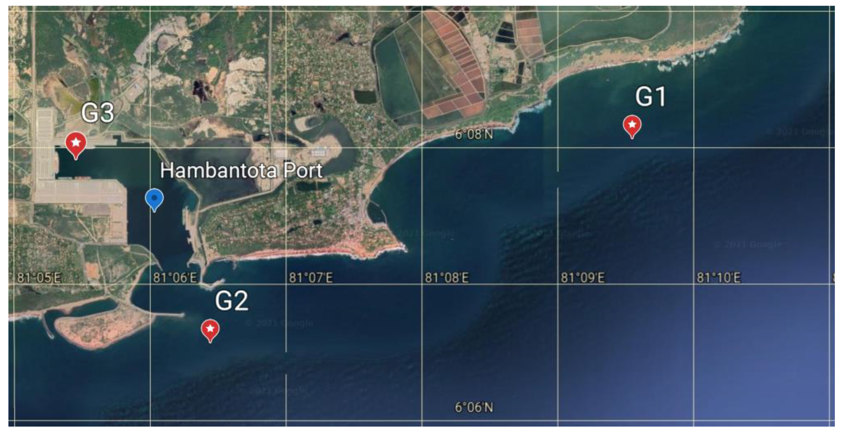
In this study, the accuracy of XB-SB in modeling IG waves inside a harbor was assessed using an in situ observation dataset. The observations were based on three sensors. Two of these were placed near the shoreline. In particular, one was fixed inside the port. Wave heights of the short and IG waves were the focus of this study. Furthermore, the impact of the grid resolution and computational domain scale on the simulation accuracy of XB-SB in modeling IG waves was investigated. The performance accuracy of XB-SB to model the natural periods of the harbor was also evaluated. This study provides a reference and guidance for further applications of XB-SB in coastal IG wave forecasting and harbor hydrodynamic simulations.

In the following section, a brief discussion on the field observations is provided. A numerical modeling approach is presented in Section 3. In addition, the post-processing of data and error metrics for evaluating the accuracy of the model are discussed. In Section 4, the model is validated using the measured data. Next, the performance of XB-SB inside the harbor is assessed, including the wave hydrodynamics and the natural periods of the port. Finally, the results of this study are discussed and the conclusions are presented.

2. Field Observations

Hambantota Port is located at the southmost tip of Sri Lanka and is an important node port on the Indian Ocean route. Its geographic location is depicted in Figure 1. Long-period waves in the port had a significant impact on the moored ships during the early stage of port completion. When the ship transporting the port crane arrived at Hambantota Port and berthed at the established berth, the crane could not be unloaded owing to the excessive movement of the ship. To study the wave characteristics of Hambantota Port, in situ wave observations were performed at the port during the southwest monsoon period (June to September) in 2018 and 2019. Water-free surface records from three sensors at three different locations were used in this study.

The placements of the three AWAC sensors are depicted as red marks in Figure 1. Sensor G1 was located near the shoreline and approximately 7 km from the harbor entrance. Sensors G2 and G3 were installed in the harbor entrance and inside the harbor, respectively. Based on the acoustic surface tracking technology, the AWAC sensors are capable of measuring the direction-resolved elevation, based on which the significant wave height and peak period can be extracted. Due to the measuring instrument itself, some unreasonable values may appear in the measured data. To correct the measured elevation, linear interpolation was performed between useful data points, whereas data with too many spikes were discarded. Details regarding the observed records are listed in

Table 1. Characteristics of observed data used in this study.

Location	Depth (m)	Start and End Dates	Duration (Day)	Measurement Setup
G1	13.05	1–25 September 2018	25	20 min/h, sampling at 2 Hz
G2	18.03	1–25 September 2019	25	34 min/h, sampling at 2 Hz
G3	17.58	1–25 September 2019	25	20 min/h, sampling at 4 Hz

.

3. Numerical Modeling

3.1. Model Description

3.1.1. Model Equations

XB-SB does not solve the short waves individually, therefore, it cannot obtain their phase information. In fact, this is valid when the study is primarily concerned with the characteristics of IG waves. XB-SB calculates short wave motions using a wave action equation with time-dependent forcing [33]. This equation solves the variation in the short wave envelope on the scale of wave groups:

$$\frac{\partial A}{\partial t}+\frac{\partial c_{x}A}{\partial y}+\frac{\partial c_{y}A}{\partial y}+\frac{\partial c_{\theta }A}{\partial \theta }=-\frac{D_w+D_f}{\sigma },$$

(1)

where wave action $A$ is given by the following equation:

$$A(x,y,t,\theta )=\frac{S_w(x,y,t,\theta )}{\sigma (x,y,t)},$$

(2)

where $c$ is the group velocity associated with the peak frequency, $\theta$ represents the angle of incidence with respect to the x-axis, and $D_w$ and $D_f$ are dissipation terms for the respective waves and bottom friction [34]; $S_w$ is the wave energy density in each directional bin, and intrinsic frequency $\sigma$ is calculated as

$$\sigma =\sqrt{gk\tanh kh}.$$

(3)

The dissipation term for the wave breaking $D_w$ is calculated as

$$D_w=\frac{2\alpha }{T_{rep}}{Q}_b{E}_w\frac{H_{rms}}{h},$$

(4)

where:

$$Q_b=1-\exp (-{(\frac{H_{rms}}{H_{\max }})}^n),$$

(5)

$$H_{rms}=\sqrt{\frac{8E_w}{\rho g}},$$

(6)

$$H_{\max }=\gamma (h+\delta H_{rms}),$$

(7)

where $\alpha$ is a wave dissipation factor, $T_{rep}$ is the mean period, $Q_b$ is a probability function (fraction of breaking waves), $E_w$ is the total short wave group energy, and $h$ is the local water depth, $\gamma$ is the breaker index.

The dissipation term for the bottom friction $D_f$ is calculated as

$$D_f=\frac{2}{3}\rho \pi f_w{\left[\frac{\pi H}{T_{rep}\sinh (kh)}\right]}^3,$$

(8)

where $f_w$ is the orbital motion friction factor, $k$ is the wave number.

The IG wave motions are solved in the time domain using the classical nonlinear shallow water equation [35] as follows:

$$\frac{\partial \eta }{\partial t}+\frac{\partial h{u}^L}{\partial x}+\frac{\partial h{v}^L}{\partial y}=0,$$

(9)

$$\frac{\partial u^L}{\partial t}+u^L\frac{\partial u^L}{\partial x}+v^L\frac{\partial u^L}{\partial y}-f{v}^L-v_h(\frac{{\partial }^2{u}^L}{\partial x^2}+\frac{{\partial }^2{u}^L}{\partial y^2})=\frac{{\tau }_{sx}}{\rho h}-\frac{{\tau }_{bx}^E}{\rho h}-g\frac{\partial \eta }{\partial x}+\frac{F_x}{\rho h},$$

(10)

$$\frac{\partial v^L}{\partial t}+u^L\frac{\partial v^L}{\partial x}+v^L\frac{\partial v^L}{\partial y}-f{u}^L-v_h(\frac{{\partial }^2{v}^L}{\partial x^2}+\frac{{\partial }^2{v}^L}{\partial y^2})=\frac{{\tau }_{sy}}{\rho h}-\frac{{\tau }_{by}^E}{\rho h}-g\frac{\partial \eta }{\partial y}+\frac{F_y}{\rho h},$$

(11)

where $u^L$ and $v^L$ represent the Lagrangian velocities, $v_h$ is the horizontal viscosity, $f$ is the Coriolis coefficient, ${\tau }_{sx}$ and ${\tau }_{sy}$ are wind shear stresses, ${\tau }_{bx}^E$ and ${\tau }_{by}^E$ are the bed shear stresses determined by the Chezy coefficient $C$. $\eta$ is the water level and $h$ is the water depth. $\rho$ represents the water density and $g$ the gravitational constant. The wave energy variation exerts a force on the water column through radiation stress gradients [36] and serves as the input for the nonlinear shallow water equation. The wave forces are given by

$$F_x=-\left[\frac{\partial S_{xx}}{\partial x}+\frac{\partial S_{xy}}{\partial y}\right],$$

(12)

$$F_y=-\left[\frac{\partial S_{yy}}{\partial y}+\frac{\partial S_{yx}}{\partial x}\right].$$

(13)

3.1.2. Boundary Conditions

The boundary conditions of the model computational domain are defined as follows:

i.

For the offshore boundary of XB-SB, a weakly reflective boundary is used where the reflected IG waves can pass through the offshore boundary with minimal reflection.

ii.

Neumann boundary conditions are used for the lateral boundaries, which indicate that there is locally no change in surface elevation and velocity.

iii.

At the seaward and landward boundary radiating boundary conditions are prescribed, taking into account the incoming bound IG waves.

XB-SB cannot specify porosity or reflection coefficients for structures, which means that porous structures such as breakwaters and quay walls are impermeable in the model. Therefore, porous structures are not taken into account in this study. XB-SB does not consider the diffraction and reflection of short waves, and the short wave energy is fully absorbed into the structures. The IG waves are considered to be fully reflected off the structures.

3.2. Numerical Setup

Two computational domains of different scales were used for the numerical simulation, as depicted in Figure 2. The size of the first computational domain (D1) was 15 km × 10 km. The objective of D1 was to reproduce the hydrodynamics of the sea area where Hambantota Port is located. The second computational domain (D2) was centered on sensor G1 and had a size of 2 km × 2.5 km. Because using D1 for model verification would consume a lot of unnecessary calculation time, we selected D2 as the computational domain for model validation. The model setups of D1 and D2 are discussed in Section 3.2.1 and Section 3.2.2, respectively.

3.2.1. Model Setup of D1

Various grid spaces were adopted for D1. The grid resolution was 8 m in and near the harbor. It gradually increased to 20 m at the boundary of the domain. The grid resolution was based on 20 grids per wavelength, which was determined using the model validation findings in Section 4.1. The shoreline used in the simulation was extracted from Google Earth, and bathymetry was obtained from the electronic chart.

At the open boundary of the computational domain, XB-SB was forced with the time-varying wave spectrum obtained from the large-scale wave prediction model WW3. The output of WW3 is a frequency-directional spectrum, with a frequency domain between 0.03 and 0.7 Hz and a directional resolution of 10°. XBeach supports spatially varying wave boundary conditions. The locations of the input spectrum are marked by red dots in Figure 2. The spatial distribution of the wave energy along the offshore boundary of the computational domain was interpolated linearly among the input spectra at discrete points. Based on a pretest (not presented herein), the simulation accuracy for D1 can be guaranteed when the number of discrete input points is greater than 4.

An automatically optimized time step was applied by XBeach, and its stability was controlled by the Courant-Friedrichs-Lewy (CFL) criterion. For the two-dimensional horizontal (2DH) simulation in this study, CFL = 0.7 was appropriate to ensure numerical convergence. Because the focus of this study was wave hydrodynamics, the sediment transport and morphology modules were switched off. The remaining parameters were set to default values of XBeach. The detailed model input parameters are listed in

Table A1. General input parameters for model D1 (D2 only has grid parameters different from D1).

Parameter	Definition	Value
nx	Number of grid cell in x-direction	1100
ny	Number of grid cell in y-direction	750
thetamin	Lower directional limit (deg)	90
thetamax	Higher directional limit (deg)	270
dtheta	Wave direction bin size (deg)	20
CFL	Courant-criterion	0.7
front, back	Flow boundary conditions	Weakly-reflective
left, right	Flow boundary conditions, lateral	Neumann
break	Short wave breaking	Roelvink2

in Appendix A.

3.2.2. Model Setup of D2

To evaluate the accuracy of XB-SB in simulating the nearshore IG waves, the model was validated by comparing the simulation results of D2 with the observations at sensor G1, which was installed near the shoreline. To determine the impact of grid resolution on the accuracy of XB-SB in modeling IG waves, three representative grid resolutions were selected, from coarse to fine, based on the rule of thumb; the detailed parameters can be found in

Table A2. Grid parameters for model D2.

	Grid 1	Grid 2	Grid 3
Grid points per wavelength	5	15	20
Grid resolution (m)	30	12	8
Number of computational grids	6216	38,272	85,800

in Appendix B. Similar to D1, D2 also used the frequency-directional spectrum from WW3 as the wave boundary condition. For the computational domain at the D2 scale, the accuracy of the simulation can be ensured by setting a single input wave spectrum at the domain boundary.

3.3. Data Analysis

Spectral analysis of the measured data was performed using the discrete Fourier transform. For simplicity, only the spectra of the three measurement points on the day when the IG wave component is significant are shown (Figure 3). The results show that the vast majority of the IG wave energy is concentrated in the range of $f$ ≤ 0.04 Hz. Therefore, in this study, the IG waves were defined as 0.005 Hz ≤ $f$ ≤ 0.04 Hz and short waves as $f$ > 0.04 Hz. The short significant wave heights and IG significant wave heights were then calculated as follows:

$$H_S=4\sqrt{{\displaystyle {\int }_{0.04}^{0.5}S(f)df}},$$

(14)

$$H_{IG}=4\sqrt{{\displaystyle {\int }_{0.005}^{0.04}S(f)df}}.$$

(15)

XB-SB does not calculate the short waves individually, and the short significant wave height $H_S$ was calculated directly from the short-wave energy. The IG significant wave height $H_{IG}$ was calculated as follows:

$$H_{IG}=4\sqrt{m_0},$$

(16)

where $m_0$ is the zero-order moment of the energy spectrum, which is obtained by calculating the variance of the long-wave surface elevation time series.

3.4. Error Metrics

In this study, the Pearson correlation coefficient (CC) was used to measure the linear dependence between the numerical results, S, and observations, O:

$$CC=\frac{{\displaystyle {\sum }_{i=1}^N((S_i-\overline{S})\cdot (O_i}-\overline{O}))}{\sqrt{{\displaystyle {\sum }_{i=1}^N{(S_i-\overline{S})}^2}}\cdot \sqrt{{\displaystyle {\sum }_{i=1}^N{(O_i-\overline{O})}^2}}},$$

(17)

where N is the number of data points. It had a value between 0 and 1, where 1 indicates a total positive linear correlation between the two variables, and 0 indicates no linear correlation.

The error between the simulated results and observed data is expressed as the relative bias (RBIAS) and normalized root mean squared error (NRMSE):

$$RBIAS=\frac{{\displaystyle {\sum }_{i=1}^N(S_i-O_i)}}{N\overline{O}},$$

(18)

$$NRMSE=\sqrt{\frac{{\displaystyle {\sum }_{i=1}^N{(S_i-O_i)}^2}}{{\displaystyle {\sum }_{i=1}^N{O}_i{}^2}}},$$

(19)

where a value closer to zero represents a better simulation.

4. Results and Discussion

4.1. Model Validation

To evaluate the accuracy of XB-SB in modeling the 2DH hydrodynamics, the simulation results of D2 were compared with the observations at sensor G1 (Figure 4). The performance statistics are presented in

Table 2. Performance statistics of XB-SB at the location of sensor G1.

	CC	RBIAS	NRMSE
$H_S$	0.73	0.0464	0.1278
$H_{IG}$	0.67	−0.1123	0.2198

. The results of the effect of grid resolution on model accuracy are shown in Appendix B (see Figure A1 and Figure A2 for $H_S$ and $H_{IG}$, respectively, and

Table A3. Performance statistics of XB-SB at the location of sensor G1.

	Grid Resolution	CC	RBIAS	NRMSE
$H_S$	dx = L/5	0.69	−0.0451	0.1343
	dx = L/15	0.70	−0.0535	0.1347
	dx = L/20	0.73	0.0464	0.1278
$H_{IG}$	dx = L/5	0.35	0.3915	0.4427
	dx = L/15	0.55	−0.0046	0.1987
	dx = L/20	0.67	−0.1123	0.2198

lists the performance statistics). The comparison results indicate that the discrepancy between the $H_S$ simulation results corresponding to the three grid resolutions is minor. Nevertheless, a discrepancy was evident for $H_{IG}$. When the grid size decreased, the model performance improved and reached the best when the grid resolution was 20 grid points per wavelength. Further tests indicated that using a grid resolution finer than 20 grid points per wavelength barely improved the accuracy of the simulation; however, it significantly increased the computation time. Therefore, a grid resolution of 20 grid points per wavelength might be appropriate when XB-SB is used to simulate nearshore IG waves.

It can be concluded from the comparison results that the 2DH hydrodynamics modeled using XB-SB are in reasonable agreement with the observations at sensor G1. This proves that the model can accurately reproduce the IG waves in the study area. It also demonstrates that WW3-XB-SB is a reliable combination to model nearshore wave hydrodynamics.

4.2. Sensitivity to Computational Domain Scale

To determine whether the scale of the computational domain affects the accuracy of XB-SB in modeling the 2DH hydrodynamics, we ran the model using both D1 and D2. The simulation results were compared with the observations recorded at sensor G1. For simplicity, the simulation period was a week in which the wave height change trend was obvious (5–13 September). Figure 5 depicts the comparison results, and

Table 3. Performance statistics for D1 and D2.

	Computational Domain	CC	RBIAS	NRMSE
$H_S$	D1	0.82	0.1082	0.1557
	D2	0.85	0.0813	0.1307
$H_{IG}$	D1	0.78	−0.2640	0.3001
	D2	0.78	−0.0324	0.1671

lists the performance statistics.

For $H_S$, the performances of D1 and D2 did not differ significantly. The results of the two domains were in good agreement with the observations, and D2 slightly outperformed D1. For $H_{IG}$, the simulation results of D1 maintained a strong correlation with the observations, yet underestimated the IG wave heights to some extent. This could be attributed to the fact that XB-SB underestimated the groupiness [37] of the short waves when modeling the wave propagation over a large distance [38]. The groupiness of short waves is responsible for forcing bound IG waves [16,20]. Under ideal conditions, the bound IG waves are linearly proportional to the groupiness. In XB-SB, the short wave groups are directional propagation in the directional bins, and the wave energy from various directional bins is simply added without considering the interaction between various wave components. This reduced the groupiness of the short waves and led to an underestimation of the bound IG waves.

In summary, using a large-scale calculational domain such as D1 (15 km × 10 km) has essentially no impact on the accuracy of XB-SB in modeling short waves. For IG waves, D1 is still able to maintain a reasonable correlation with the field observations. Although the IG wave heights were somewhat underestimated, the overall error was within acceptable limits. The above conclusions demonstrate that XB-SB is capable of performing hydrodynamic simulations over a large study area. Furthermore, it is appropriate to use D1 to investigate the performance of the XB-SB in modeling the IG waves inside and outside Hambantota Port.

4.3. Performance on Harbor

4.3.1. Infragravity Waves near Harbor Entrance

The performance of XB-SB in modeling IG waves near a port is assessed in this section. Figure 6 depicts a comparison of the significant wave heights modeled using XB-SB with the observations at sensor G2. Note that sensor G2 was deployed in front of the harbor and near the entrance. Therefore, the wave characteristics at this location can be used as a reference for the incoming wave at the port.

It is evident from Figure 6 that the results of XB-SB correlate strongly with the in situ observations for both short waves and IG waves.

Table 4. Performance statistics of XB-SB at the location of sensor G2.

	CC	RBIAS	NRMSE
$H_S$	0.70	−0.0498	0.1409
$H_{IG}$	0.62	−0.0567	0.3710

presents the performance statistics. For the IG wave heights focused on in this study, the accuracy of XB-SB appeared to be somewhat reduced. The error might have resulted from XB-SB not considering the outgoing waves from the port. However, the results generally were in good agreement with the observations. Note that there were some unexpected great peaks on certain dates (e.g., 13 and 21 September), which remain to be determined in future studies.

In general, the hydrodynamics outside the port can be reproduced accurately using XB-SB. For IG wave heights near the harbor entrance, XB-SB can provide a reliable and crude estimation, which is crucial for assessing the performance of the model in modeling IG waves inside the harbor.

4.3.2. Infragravity Waves Inside Harbor

Based on the above studies, the performance of XB-SB in modeling the hydrodynamics in the harbor is assessed in this section. Figure 7 illustrates the comparison of the observed and modeled significant wave heights at sensor G3, and

Table 5. Performance statistics of XB-SB at the location of sensor G3.

	CC	RBIAS	NRMSE
$H_S$	0.32	−0.9960	0.9961
$H_{IG}$	0.46	1.3760	1.7541

lists the performance statistics.

These results were somewhat surprising. For short waves, XB-SB seriously underestimated the wave height at all times. As is evident in Figure 7a, it seems that there is no short wave at the location of sensor G3. Although the data in Table 5 indicate that the simulation results and the observations maintain a valid correlation, the error is unacceptable. The reason for this poor result is that XB-SB did not consider diffraction and reflection, which are significant for the propagation of short waves in the harbor. This resulted in a significant error between the modeled and observed wave heights. Contrary to the results for short waves, the IG waves in the harbor were generally overestimated by XB-SB and severely overestimated on some dates (e.g., 13–19 September), as depicted in Figure 7b.

For a visual illustration, the wave height distribution with a zoom on Hambantota Port is depicted in Figure 8. It is evident that the short wave heights decreased rapidly as soon as the short waves reached the harbor (see Figure 8a). Note that Hambantota Port is well sheltered by the breakwater and revetment. Therefore, the waves can hardly propagate directly into the interior of the harbor basin. Nevertheless, the two main methods of diffraction and reflection for short waves propagation in the port have not been considered by XB-SB. Therefore, the vast majority of short waves are absorbed by the boundary after entering the harbor basin. Almost no short waves can propagate to the area in front of the quay where sensor G3 is located. This explains the significant underestimation of the short wave heights in Figure 7a. However, the overestimation of IG waves in the harbor was unexpected. Probably, this anomalous performance of IG waves inside the port is related to the absence of short wave energy; however, no convincing explanation for this was found in this study.

In summary, XB-SB evidently underestimated the short wave heights in Hambantota Port, particularly in the obscured areas and corners. The corresponding IG wave heights were overestimated. Hambantota Port is well sheltered by breakwaters. Therefore, an accurate reproduction of the hydrodynamics of Hambantota Port is extremely difficult for XB-SB, which does not consider the diffraction and reflection of short waves.

4.3.3. Natural Periods of the Port

The natural period is a fundamental parameter of a given harbor and does not change with the wave state. Dong [11] found that the Hambantota Port has four natural periods, which are 400 s, 173 s, 52 s, and 35 s. To investigate whether XB-SB can capture the natural period of the Hambantota Port, a spectral analysis of the simulation results was performed at the location of sensor G3. For simplicity, two representative dates were selected for the investigation, namely 16 September, when the IG wave component was significant, and 8 September, when the IG wave component was not significant. The spectra were shown in Figure 9, and

Table 6. Natural periods from measurement and numerical simulation.

	Mode 1	Mode 2	Mode 3	Mode 4
Measurement	400 s	173 s	52.0 s	35.0 s
Simulation 8 September	454 s	170 s	53.0 s	32.0 s
Simulation 16 September	484 s	168 s	57.0 s	34.0 s

lists the natural periods obtained from the measurement and numerical simulation. It can be seen from the comparison results that XB-SB somewhat overestimates mode1, and the remaining three modes are in agreement with the measured results. In general, the natural periods of the Hambantota Port can be reliably estimated by XB-SB.

5. Conclusions

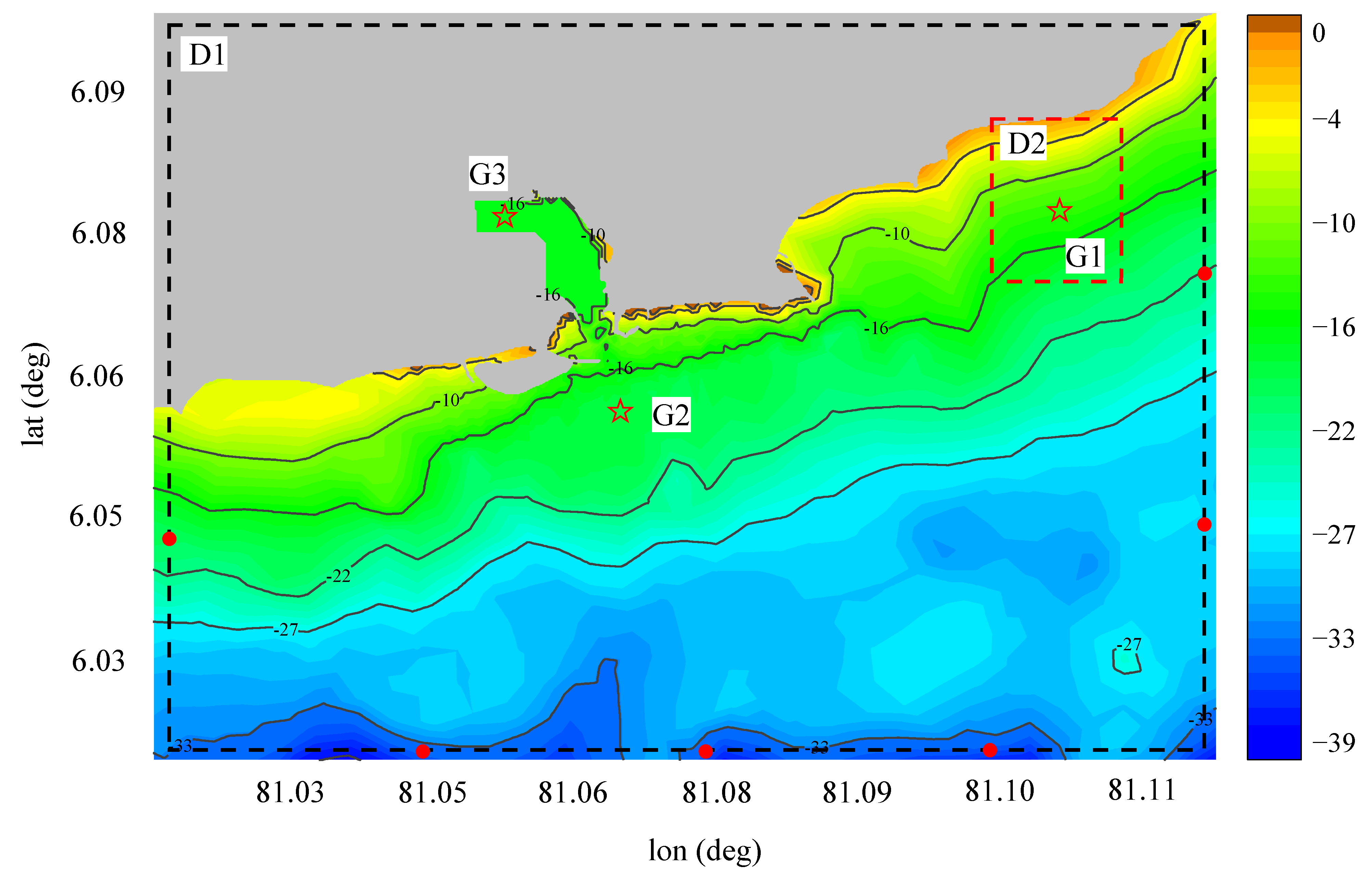
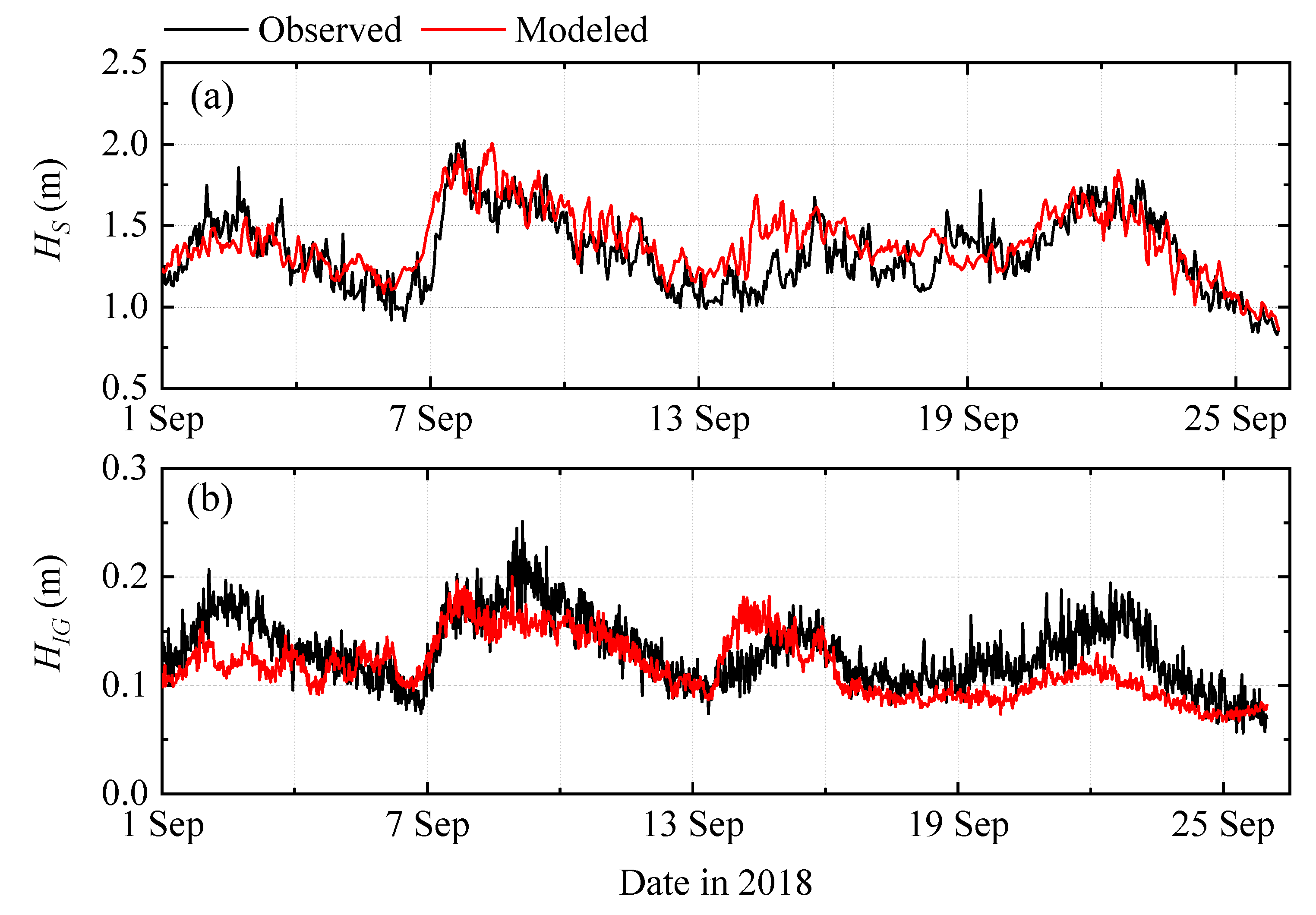
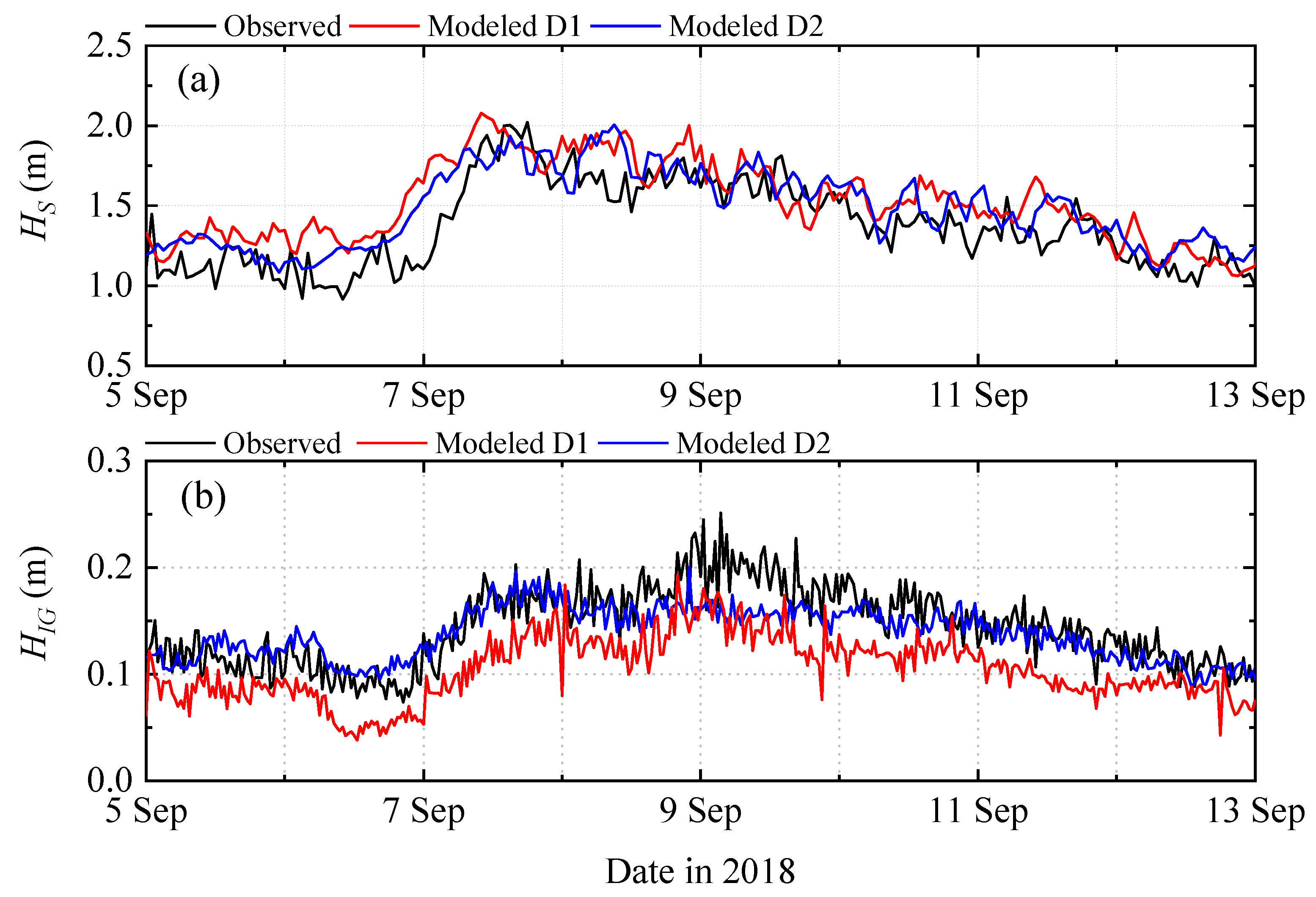
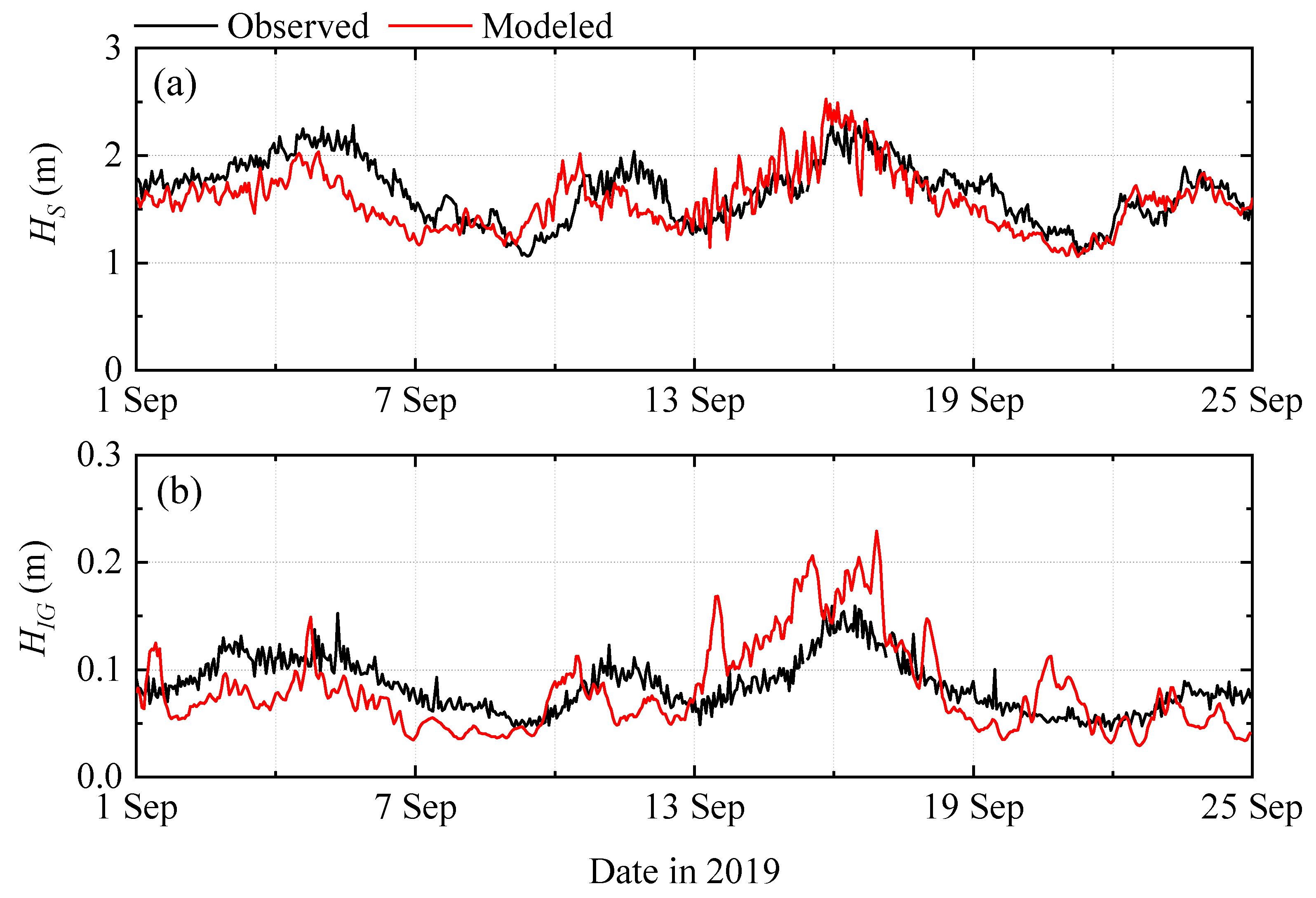
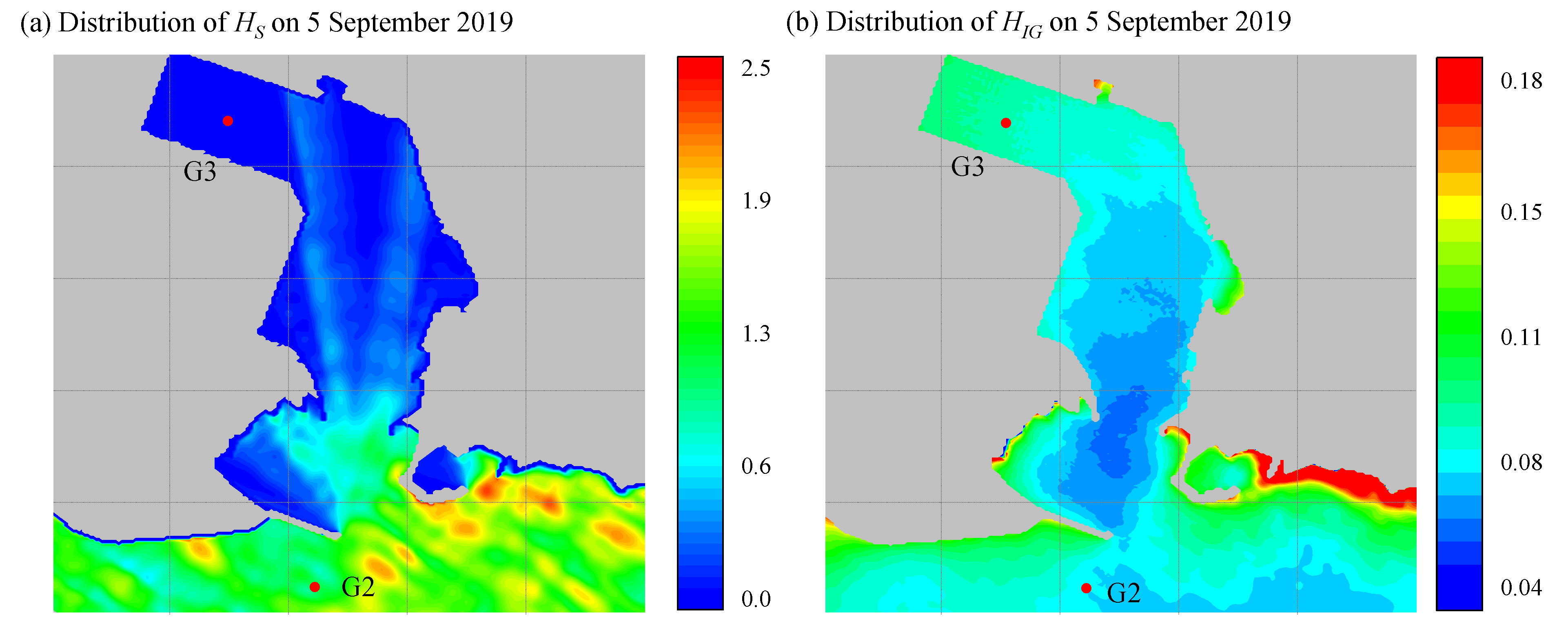
The accuracy of the wave-group-resolving model XB-SB in modeling the IG waves in a port was assessed by comparisons with field measurements obtained at Hambantota Port located in Sri Lanka. Two computational domains of various scales (D1: 15 km × 10 km; D2: 2 km × 2.5 km) were used in the numerical simulations. The objective of D1 was to reproduce the hydrodynamics of the sea area where Hambantota Port is located. Domain D2 was used for model verification. The model was validated by comparing the simulation results of D2 with the observations at sensor G1 installed at the shoreline. An appropriate grid resolution for nearshore IG wave simulations using XB-SB was used. To investigate the impact of the use of a large range of computational domains on the accuracy of XB-SB in modeling IG waves, the model was also validated using D1 and compared with the results of D2.

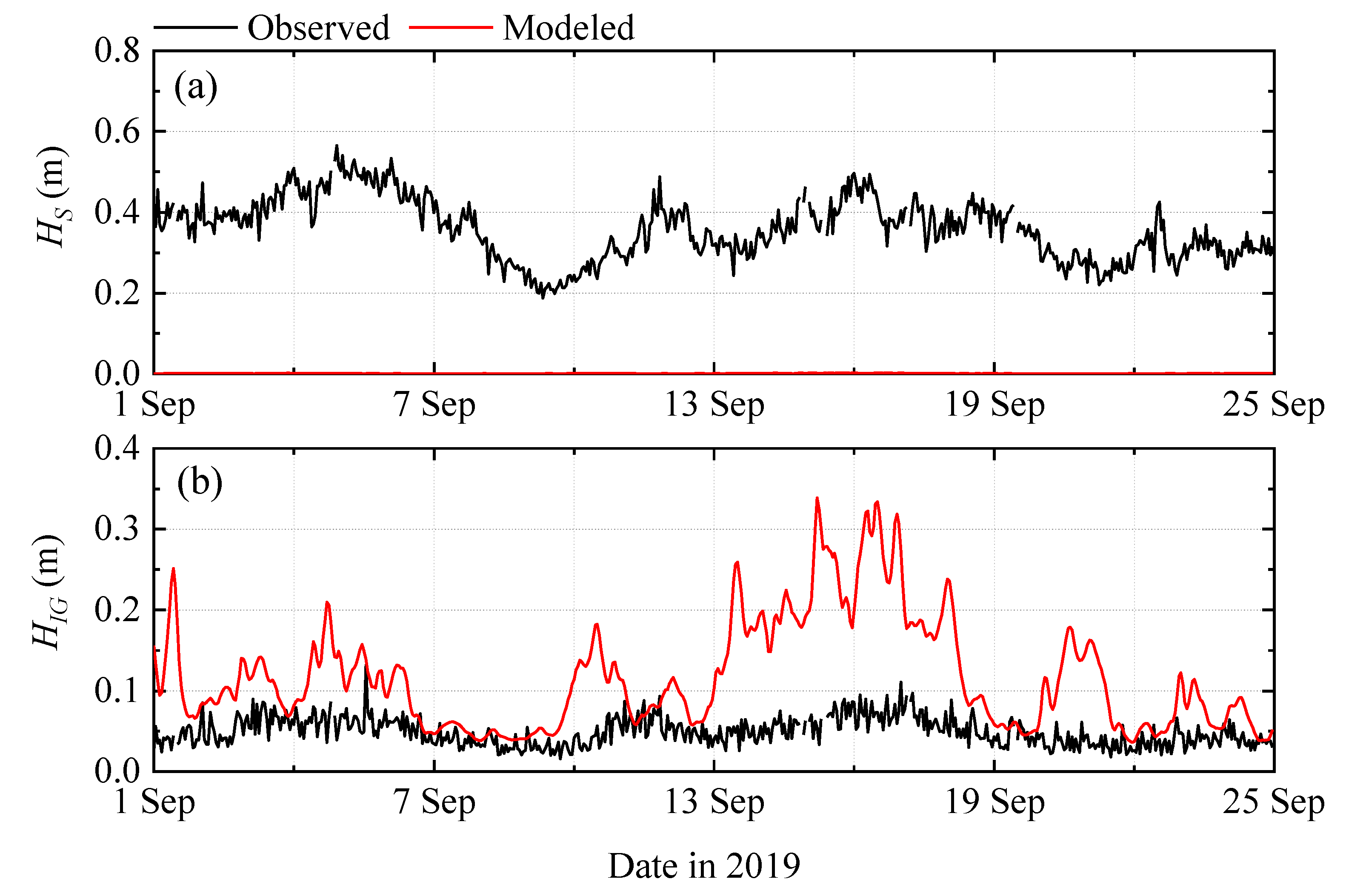
Next, the accuracy of XB-SB in modeling the IG waves near and inside the harbor was assessed by comparing the model results with observations from two sensors installed in and outside Hambantota Port. The performance of the model in calculating the natural periods of the harbor was also evaluated.

The conclusions of this study are as follows:

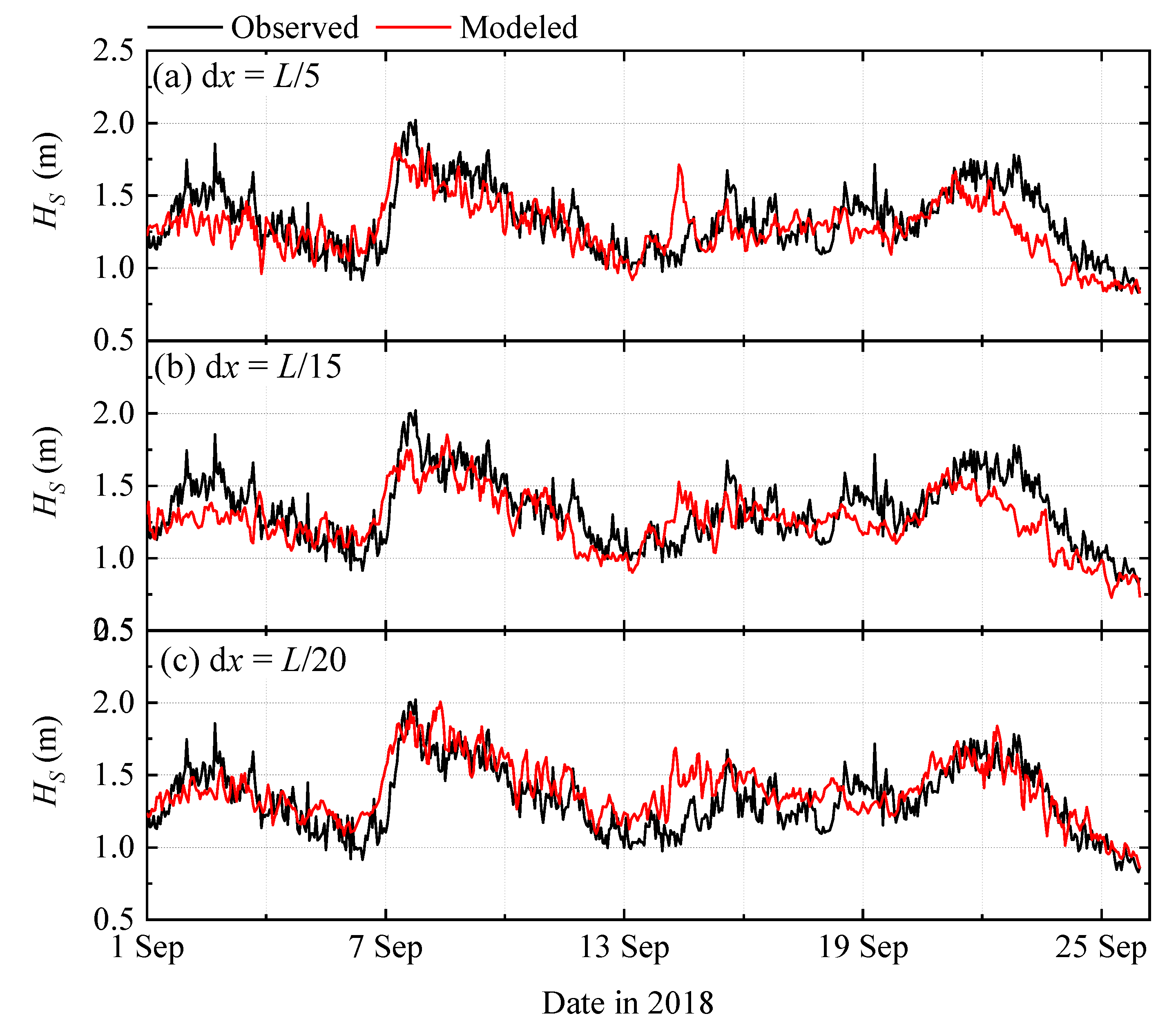
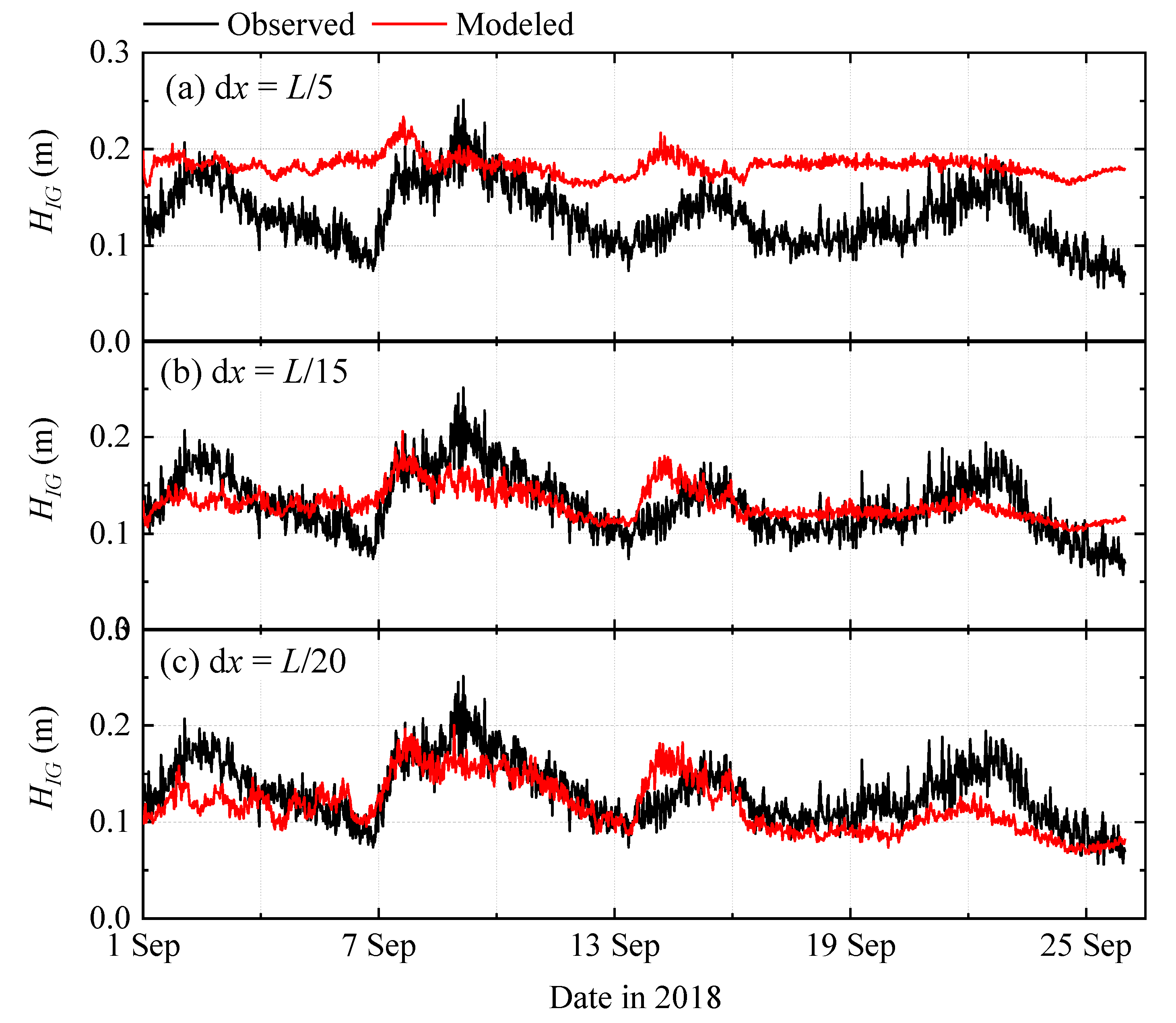
• XB-SB can accurately predict the short and IG wave heights in an open domain without obstacles. The use of a grid resolution of 20 grid points per wavelength is recommended to simulate nearshore IG waves using XB-SB.
• XB-SB is capable of reproducing large-scale hydrodynamics. Because the model does not fully consider the IG waves generated by the groupiness of short waves, the IG wave height is slightly underestimated when simulations are performed using a large-scale (such as 15 km × 10 km) computational domain.
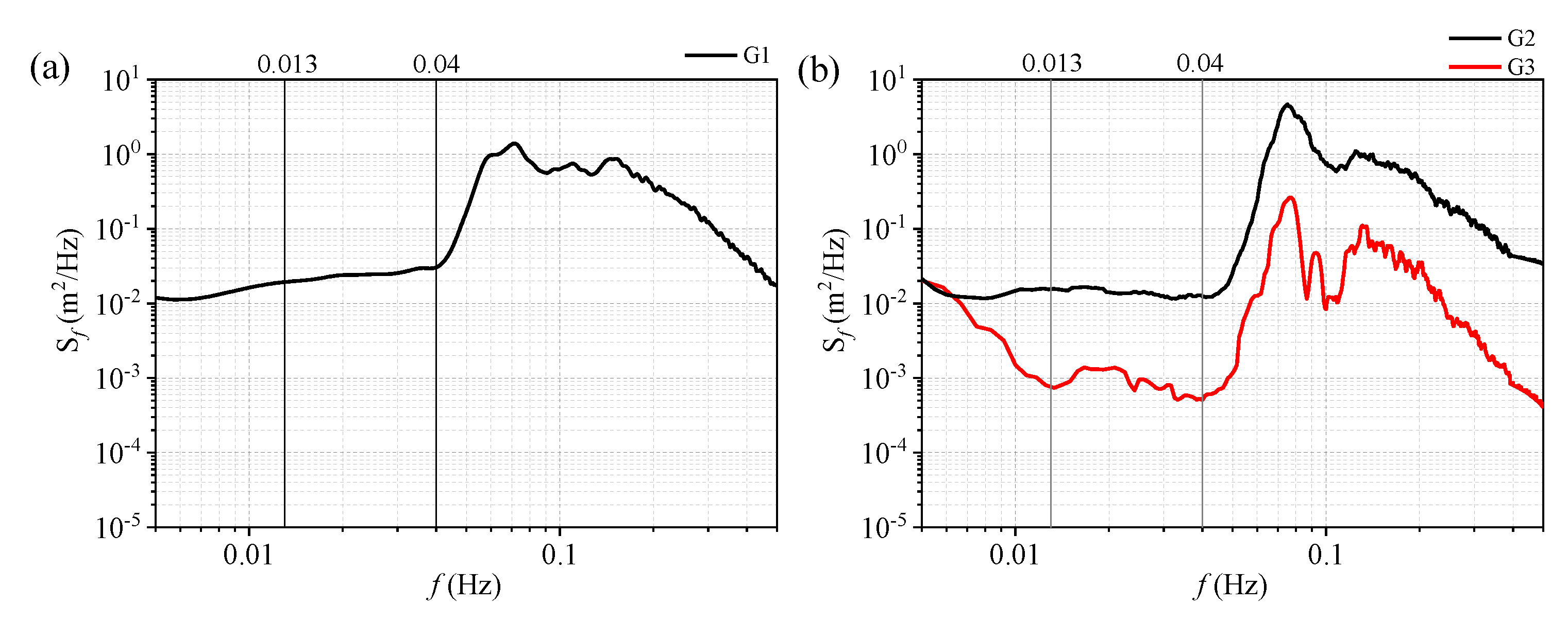
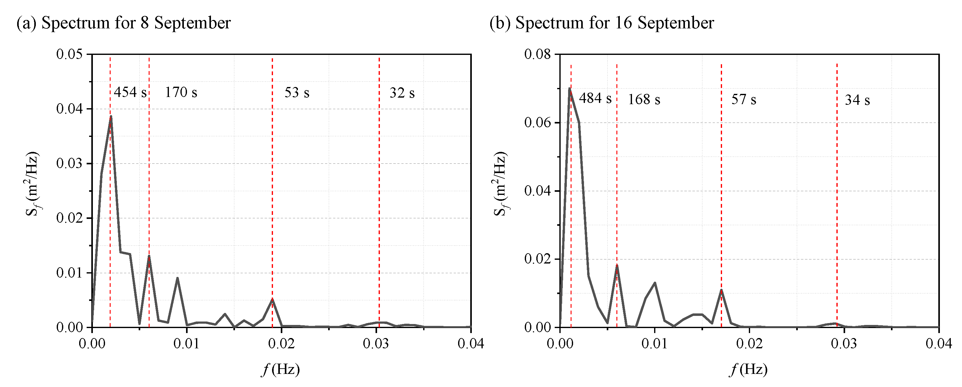
• For the area near the entrance of a port like Hambantota Port, XB-SB can accurately predict the wave heights of both short and IG waves. However, a large error occurs inside the harbor. The short wave heights inside the harbor are significantly underestimated because XB-SB does not consider the diffraction and reflection of short waves. For IG waves inside the port, a correlation exists between the simulation results and observations. However, in general, XB-SB overestimates the IG wave heights. The natural periods of the Hambantota Port are well identified by XB-SB.

In general, XB-SB can be used to reproduce large-scale hydrodynamics and provide accurate predictions for nearshore IG waves. However, it is not appropriate to use it to simulate the hydrodynamics inside a harbor like Hambantota Port, which is well sheltered and where it is difficult for waves to propagate directly into the harbor basin. XB-SB is still a promising tool for predicting IG waves inside a harbor when the diffraction and reflection of short waves can be considered.

References

1. Munk, W.H. Surf beats. Eos Trans. Am. Geophys. Union 1949, 30, 849–854. [Google Scholar]
2. Roelvink, J.A.; Stive, M.J.F. Bar-generating cross-shore flow mechanisms on a beach. J. Geophys. Res. Space Phys. 1989, 94, 4785–4800. [Google Scholar] [CrossRef]
3. Cheriton, O.M.; Storlazzi, C.D.; Rosenberger, K.J. Observations of wave transformation over a fringing coral reef and the importance of low-frequency waves and offshore water levels to runup, overwash, and coastal flooding. J. Geophys. Res. Oceans 2016, 121, 3121–3140. [Google Scholar] [CrossRef] [Green Version]
4. Gent, M.R.V. Wave runup on dikes with shallow foreshores. J. Waterw. Port Coast. Ocean. Eng. 2001, 127, 254–262. [Google Scholar] [CrossRef]
5. Sheremet, A.; Staples, T.; Ardhuin, F.; Suanez, S.; Fichaut, B. Observations of large infragravity wave runup at Banneg Island, France. Geophys. Res. Lett. 2014, 41, 976–982. [Google Scholar] [CrossRef]
6. Van Thiel de Vries, J.S.M.; Van Gent, M.R.A.; Walstra, D.J.R.; Reniers, A.J.H.M. Analysis of dune erosion processes in large-scale flume experiments. Coast. Eng. 2008, 55, 1028–1040. [Google Scholar] [CrossRef]
7. Roelvink, D.; Reniers, A.; van Dongeren, A.; Vries, J.T.; McCall, R.; Lescinski, J. Modelling storm impacts on beaches, dunes and barrier islands. Coast. Eng. 2009, 56, 1133–1152. [Google Scholar] [CrossRef]
8. Baumann, J.; Chaumillon, E.; Bertin, X.; Schneider, J.-L.; Guillot, B.; Schmutz, M. Importance of infragravity waves for the generation of washover deposits. Mar. Geol. 2017, 391, 20–35. [Google Scholar] [CrossRef]
9. McCall, R.; Vries, J.V.T.D.; Plant, N.; Van Dongeren, A.; Roelvink, J.; Thompson, D.; Reniers, A. Two-dimensional time dependent hurricane overwash and erosion modeling at Santa Rosa Island. Coast. Eng. 2010, 57, 668–683. [Google Scholar] [CrossRef]
10. Chen, G.-Y.; Chien, C.-C.; Su, C.-H.; Tseng, H.-M. Resonance induced by edge waves in Hua-Lien Harbor. J. Oceanogr. 2004, 60, 1035–1043. [Google Scholar] [CrossRef]
11. Dong, G.; Zheng, Z.; Ma, X.; Huang, X. Characteristics of low-frequency oscillations in the Hambantota Port during the southwest monsoon. Ocean Eng. 2020, 208, 107408. [Google Scholar] [CrossRef]
12. Van Der Molen, W.; Monárdez, P.; Van Dongeren, A. Numerical simulation of long-period waves and ship motions in Tomakomai Port, Japan. Coast. Eng. J. 2006, 48, 59–79. [Google Scholar] [CrossRef]
13. Rabinovich, A. Chapter 9: Seiches and harbor oscillations. In Handbook of Coastal and Ocean Engineering; Kim, Y.C., Ed.; World Scientific Publishing: Singapore, 2009; pp. 193–236. [Google Scholar]
14. Zheng, Z.; Ma, X.; Ma, Y.; Dong, G. Wave estimation within a port using a fully nonlinear Boussinesq wave model and artificial neural networks. Ocean Eng. 2020, 216, 108073. [Google Scholar] [CrossRef]
15. Tucker, M.J. Surf beats: Sea waves of 1 to 5 min. period. Proc. R. Soc. Lond. Ser. A Math. Phys. Sci. 1950, 202, 565–573. [Google Scholar]
16. Longuet-Higgins, M.S.; Stewart, R.W. Radiation stress and mass transport in gravity waves, with application to ‘surf beats’. J. Fluid Mech. 1962, 13, 481–504. [Google Scholar] [CrossRef]
17. Huntley, D.A.; Guza, R.T.; Thornton, E.B. Field observations of surf beat: 1. Progressive edge waves. J. Geophys. Res. Space Phys. 1981, 86, 6451–6466. [Google Scholar] [CrossRef]
18. List, J.H. A model for the generation of two-dimensional surf beat. J. Geophys. Res. Space Phys. 1992, 97, 5623. [Google Scholar] [CrossRef]
19. Masselink, G. Group bound long waves as a source of infragravity energy in the surf zone. Cont. Shelf Res. 1995, 15, 1525–1547. [Google Scholar] [CrossRef]
20. Symonds, G.; Huntley, D.A.; Bowen, A.J. Two-dimensional surf beat: Long wave generation by a time-varying breakpoint. J. Geophys. Res. Space Phys. 1982, 87, 492. [Google Scholar] [CrossRef] [Green Version]
21. Agnon, Y.; Sheremet, A. Stochastic nonlinear shoaling of directional spectra. J. Fluid Mech. 1997, 345, 79–99. [Google Scholar] [CrossRef] [Green Version]
22. Zijlema, M.; Stelling, G.; Smit, P. SWASH: An operational public domain code for simulating wave fields and rapidly varied flows in coastal waters. Coast. Eng. 2011, 58, 992–1012. [Google Scholar] [CrossRef]
23. Shi, F.; Kirby, J.T.; Harris, J.; Geiman, J.D.; Grilli, S.T. A high-order adaptive time-stepping TVD solver for Boussinesq modeling of breaking waves and coastal inundation. Ocean Model. 2012, 43–44, 36–51. [Google Scholar] [CrossRef]
24. Booij, N.; Ris, R.C.; Holthuijsen, L.H. A third-generation wave model for coastal regions: 1. Model description and validation. J. Geophys. Res. Ocean. 1999, 104, 7649–7666. [Google Scholar] [CrossRef] [Green Version]
25. Tolman, H.L. User manual and system documentation of WAVEWATCH III TM version 3.14. Tech. Note MMAB Contrib. 2009, 276, 220. [Google Scholar]
26. Rijnsdorp, D.P.; Reniers, A.; Zijlema, M. (Marcel) Source code of the SWAN model: Free infragravity waves in the North Sea. J. Geophys. Res. Ocean. 2021. [Google Scholar] [CrossRef]
27. Rawat, A. Numerical Modelling of Infragravity Waves: From Regional to Global Scales. Ph.D. Thesis, University of Western Brittany, Brest, France, February 2015. Available online: https://archimer.ifremer.fr/doc/00498/60937/64330.pdf (accessed on 20 August 2021).
28. de Beer, A.; McCall, R.; Long, J.; Tissier, M.; Reniers, A. Simulating wave runup on an intermediate–reflective beach using a wave-resolving and a wave-averaged version of XBeach. Coast. Eng. 2021, 163, 103788. [Google Scholar] [CrossRef]
29. Drost, E.J.; Cuttler, M.; Lowe, R.; Hansen, J. Predicting the hydrodynamic response of a coastal reef-lagoon system to a tropical cyclone using phase-averaged and surfbeat-resolving wave models. Coast. Eng. 2019, 152, 103525. [Google Scholar] [CrossRef]
30. Lashley, C.H.; Bertin, X.; Roelvink, D.; Arnaud, G. Contribution of infragravity waves to run-up and overwash in the pertuis breton embayment (France). J. Mar. Sci. Eng. 2019, 7, 205. [Google Scholar] [CrossRef] [Green Version]
31. Van Dongeren, A.; Lowe, R.; Pomeroy, A.; Trang, D.M.; Roelvink, D.; Symonds, G.; Ranasinghe, R. Numerical modeling of low-frequency wave dynamics over a fringing coral reef. Coast. Eng. 2013, 73, 178–190. [Google Scholar] [CrossRef]
32. Wong, A. Wave Hydrodynamics in Ports: Numerical Model Assessment of XBeach. Master’s Thesis, Delft University of Technology, Delft, The Netherlands, October 2016. Available online: https://repository.tudelft.nl/islandora/object/uuid%3A533ad406-9d7f-44bb-ba3b-7fe60e112432 (accessed on 20 August 2021).
33. Holthuijsen, L.; Booij, N.; Herbers, T. A prediction model for stationary, short-crested waves in shallow water with ambient currents. Coast. Eng. 1989, 13, 23–54. [Google Scholar] [CrossRef]
34. Daly, C.J.; Roelvink, D.; Van Dongeren, A.; Vries, J.V.T.D.; McCall, R. Short wave breaking effects on low frequency waves. Coast. Eng. Proc. 2011. [Google Scholar] [CrossRef] [Green Version]
35. Phillips, O. The Dynamics of the Upper Ocean; Cambridge University Press: London, UK; New York, NY, USA; Melbourn, UK, 1977; p. 366. [Google Scholar]
36. Longuet-Higgins, M.; Stewart, R. Radiation stresses in water waves; a physical discussion, with applications. Deep Sea Res. Oceanogr. Abstr. 1964, 11, 529–562. [Google Scholar] [CrossRef]
37. Funke, E.; Mansard, E. On the synthesis of realistic sea states. In Proceedings of the 17th International Conference on Coastal Engineering, Sydney, Australia, 23–28 March 1980; pp. 2974–2991. [Google Scholar]
38. Roelvink, D.; McCall, R.; Mehvar, S.; Nederhoff, K.; Dastgheib, A. Improving predictions of swash dynamics in XBeach: The role of groupiness and incident-band runup. Coast. Eng. 2018, 134, 103–123. [Google Scholar] [CrossRef]
Figure 1. Google Earth screenshot depicting the locations of Hambantota Port and three acoustic waves and current (AWAC) sensors. Sensor G1 is located near the shoreline, approximately 7 km from G2, located near the port entrance. Sensor G3 is deployed inside the harbor.
Jmse 09 00918 g001
Figure 2. Computational domains used in the numerical simulation: D1 (within the black dotted line) and D2 (within the red dotted line). AWAC sensors are depicted as red stars, and the red dots represent the input positions of the wave spectra obtained from WW3.
Jmse 09 00918 g002
Figure 3. Day-averaged spectra at the location of three sensors: (a) sensor G1 and (b) sensor G2 (black) and sensor G3 (red).
Jmse 09 00918 g003
Figure 4. Modeled (red) and observed (black) wave heights 1–25 September 2018, at the location of sensor G1: (a) significant wave height H S and (b) significant IG wave height H I G .
Jmse 09 00918 g004
Figure 5. Significant wave heights modeled by D1 and D2, 5–13 September 2018, at the location of sensor G1. (a) Significant short wave height H S and (b) significant IG wave height H I G .
Jmse 09 00918 g005
Figure 6. Modeled (red) and observed (black) wave heights 1–25 September 2019, at the location of sensor G2: (a) significant wave height H S and (b) significant IG wave height H I G .
Jmse 09 00918 g006
Figure 7. Modeled (red) and observed (black) wave heights 1–25 September 2019, at the location of sensor G3: (a) significant wave height H S and (b) significant IG wave height H I G .
Jmse 09 00918 g007
Figure 8. Modeled local significant wave height distributions: (a) short waves and (b) IG waves. The wave heights are the average for 5 September 2019.
Jmse 09 00918 g008
Figure 9. Modeled day-averaged spectra at location sensor G3: (a) 8 September and (b) 16 September.
Jmse 09 00918 g009