Time-Scale Decomposition Techniques Used in the Ship Path-Following Problem with Rudder Roll Stabilization Control

Abstract

The motion control of a surface ship based on a four degrees of freedom (4-DoF) (surge, sway, roll, and yaw) maneuvering motion model is studied in this paper. A time-scale decomposition method is introduced to solve the path-following problem, implementing Rudder Roll Stabilization (RRS) at the same time. The control objectives are to let the ship to track a predefined curve path under environmental disturbances, and to reduce the roll motion at the same time. A singular perturbation method is used to decouple the whole system into two subsystems of different time scales: the slow path-following subsystem and the fast roll reduction subsystem. The coupling effect of the two subsystems is also considered in this framework of analysis. RRS control is only possible when there is the so-called bandwidth separation characteristic in the ship motion system, which requires a large bandwidth separation gap between the two subsystems. To avoid the slow subsystem being affected by the wave disturbances of high frequency and large system uncertainties, the $L_1$ adaptive control is introduced in the slow subsystem, while a Proportion-Differentiation (PD) control law is adopted in the fast roll reduction subsystem. Simulation results show the effectiveness and robustness of the proposed control strategy.

1. Introduction

The path-following and roll reduction are two important control objectives in ship motion control problems. Traditionally, the path-following problem and roll reduction problem are studied separately, due to the fact that they have totally different control objectives and strategies. In path-following problem, the rudder is usually the only control input if the propeller revolution is constant. However, in the roll reduction problem, additional devices are usually used to provide effective roll reduction; for example, moving weights [1], anti-rolling tanks [2], bilge keels [3], gyroscopic stabilizers [4], and stabilizing fins [5] were widely studied and used as roll reduction devices.

Rudders are designed to control the heading and position of a ship, to make the ship move along the given course, or turn when required. In the process of course-keeping or path-following, the relatively small rudder force often limits the use of the rudder in roll reduction control, mainly due to the following facts: firstly, the slew rate saturation of the steering gear makes it difficult to control the high-frequency roll motion; secondly, the high-frequency rudder operation may cause the wear and tear of the rudder; thirdly, the fast rudder operation may affect the course-keeping or path-following performance.

Despite the above limitations, for a long time the Rudder Roll Stabilization (RRS) control system has attracted great interest from the ship motion control community. This is mainly because the RRS control system does not need any additional expensive devices, thus is cheap and convenient. In the 1980s, the basic RRS control strategies were put forward by Källström [6], Van der Klugt [7], Källström et al. [8]. During the 1990s, more advanced control laws and analyses were presented by Blanke et al. [9], Van Amerongen et al. [10], Blanke and Christensen [11], Lauvdal and Fossen [12]. In the last two decades, Perez [13], Perez and Blanke [14] carried out a comprehensive study on RRS in the course-keeping problem; Ren et al. [15] introduced singular perturbation method for the RRS problem.

Nowadays, by designing a more powerful rudder, it is possible for the rudder to have a large enough bandwidth to control the high-frequency roll motion. On the other hand, the RRS control should only be used in some emergency situations, such as when the ship encounters severe wave disturbances which may cause a dangerous roll motion. For the most time, the RRS control is not used, thus the wear and tear problem is very limited. It is well known that there exists the so-called bandwidth separation characteristic in many of the four degrees of freedom (4-DoF) (surge, sway, roll, and yaw) motion systems of surface ships [14,16]. This bandwidth separation characteristic guarantees that there is a large enough bandwidth separation gap between the yaw motion system and the roll motion system, thus the control input in a system has a very limited interference effect on the other system.

The study on RRS control system may be traced back to the pioneering work by Cowley and Lambert [17], and the original research on the design of RRS was carried out mainly in the 1980s. The studies that were the basis for real implementations can be found in Källstrom [6], Van der Klugt [7], Van Amerongen et al. [10], Blanke et al. [9,18], Grimble et al. [19], Lauvdal and Fossen [12], and Crossland [20], among others. In these studies, however, the control objective was limited to RRS control in the course-keeping problem. During the last two decades, the roll reduction control in the path-following problem has drawn a lot of interest from the ship motion control community. Most of the analyses are in the time-domain framework, where the state space equations are given and the details of the system information can be tracked. Besides, the stability analysis can also be conducted in the time domain. Fang and Luo [21] studied the track-keeping problem with roll reduction control by using separated sliding mode controllers. Li et al. [22] considered the roll angle constraints in the path-following problem by using the model predictive control (MPC) approach. Liu et al. [23] combined the line-of-sight strategy and the MPC method to the roll control in the path-following problem. However, most of the studies used the separated model of the 4-DoF ship motion system, and there were seldom an analytical framework and techniques to handle the coupling effects between the roll motion and the maneuvering motion in the horizontal plane. Few studies concentrated on the analysis of the 4-DoF ship motion system with different time-scale characteristics.

In this paper, a time-scale decomposition method is introduced to the RRS control system in the path-following problem, where the rudder is the only input for both the heading control and the roll reduction control. The time-scale analysis strategy offers a new analytical framework for considering the coupling effects of the 4-DoF ship motion system. This technique is used to decouple the ship motion system into a subsystem of slow heading control and a subsystem of fast roll motion control. The coupling effects between the two subsystems of different time scales are taken into account, which is of great importance in a path-following problem.

It is well known that the roll motion is generally much faster than the motions of other DoFs. The interaction between the opposite effects of fast and slow dynamic systems causes the non-minimum phase (NMP) phenomenon in the 4-DoF ship motion system. The NMP system has an inverse initial response and a large phase lag, which is considered as a major challenge for RRS control system design [13,24]. In this paper, a time-scale analysis technique based on a singular perturbation strategy is used to decouple the motions of different time scales. The possibility for the singular perturbation method being used in the RRS control system in course-keeping problems has been explored in the previous study [15]. In this paper, the singular perturbation equations are introduced to describe the 4-DoF motion of a surface ship in the path-following problem with RRS control.

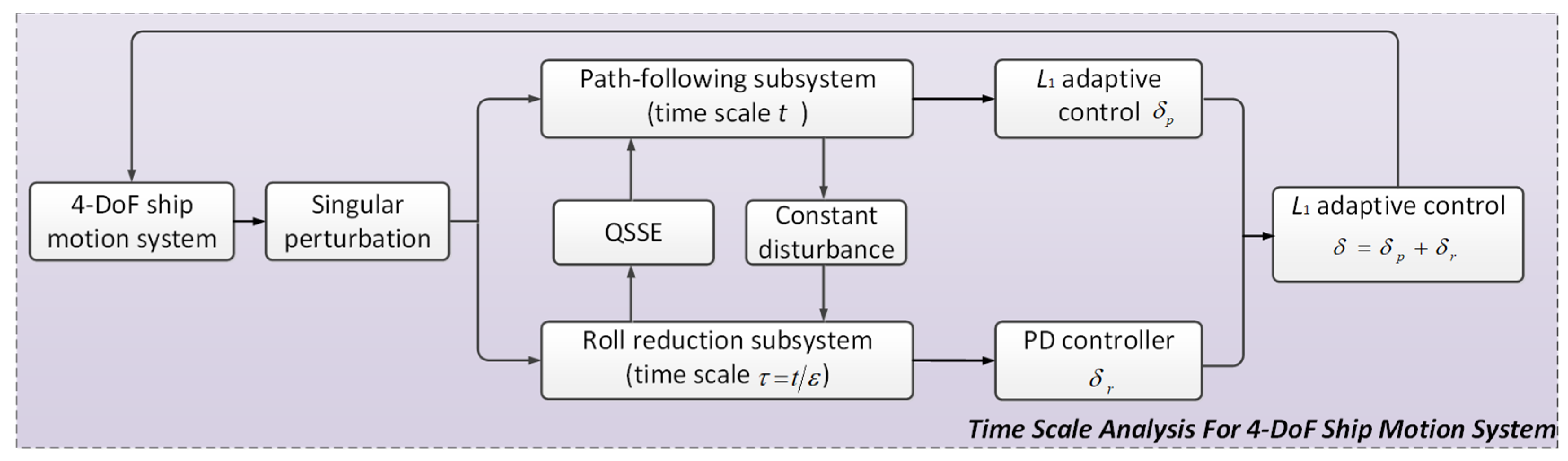
The overall scheme of the time-scale analysis is shown in Figure 1. By following the standard singular perturbation procedures, the whole system is decoupled into two subsystems of different time scales, namely the slow path-following subsystem and the fast roll motion subsystem. A new time scale τ is introduced to describe the roll motion subsystem. Under such a time scale, the coupling effect from the slow subsystem can be regarded as a constant disturbance to the fast subsystem. The so-called quasi-steady-state equilibrium (QSSE) is introduced to pass information between the subsystems of different time scales. The control objectives and strategies of these two subsystems are treated separately, and the overall control input is set as the sum of the rudder commands of these two subsystems.

Different from the typical course-keeping problem, the RRS control in the path-following problem is much more complicated. Due to the complex curve path tracking motion and time-varying wave disturbances, large uncertainties of the model and its parameters are added into the motion system. Enough input bandwidth separation should be guaranteed to avoid the interference between different subsystems in the RRS control system [15], which is particularly difficult during the path-following problem. In reality, the fast time-varying wave disturbances may cause the slow motion of some high-frequency components; if these high-frequency components are fed into the slow path-following subsystem, the control performance of the fast roll motion will be severely affected [25]. Thus, to gain good performances in both of the two time-scale subsystems, the control strategy in the slow path-following subsystem is most important.

To deal with this system uncertainty and filter the high-frequency disturbances in the slow subsystem, the $L_1$ adaptive control strategy is introduced. It was first introduced in aircraft control community [26]. This adaptive control strategy has a fast adaption speed and is applicable for systems with a large system uncertainty and time-varying characteristics. It has been introduced to the field of ship motion control in recent years [27,28,29], but has not yet been used for RRS control.

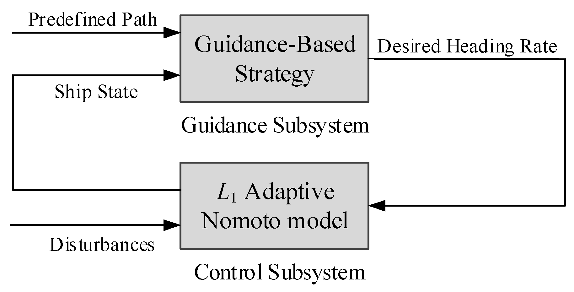
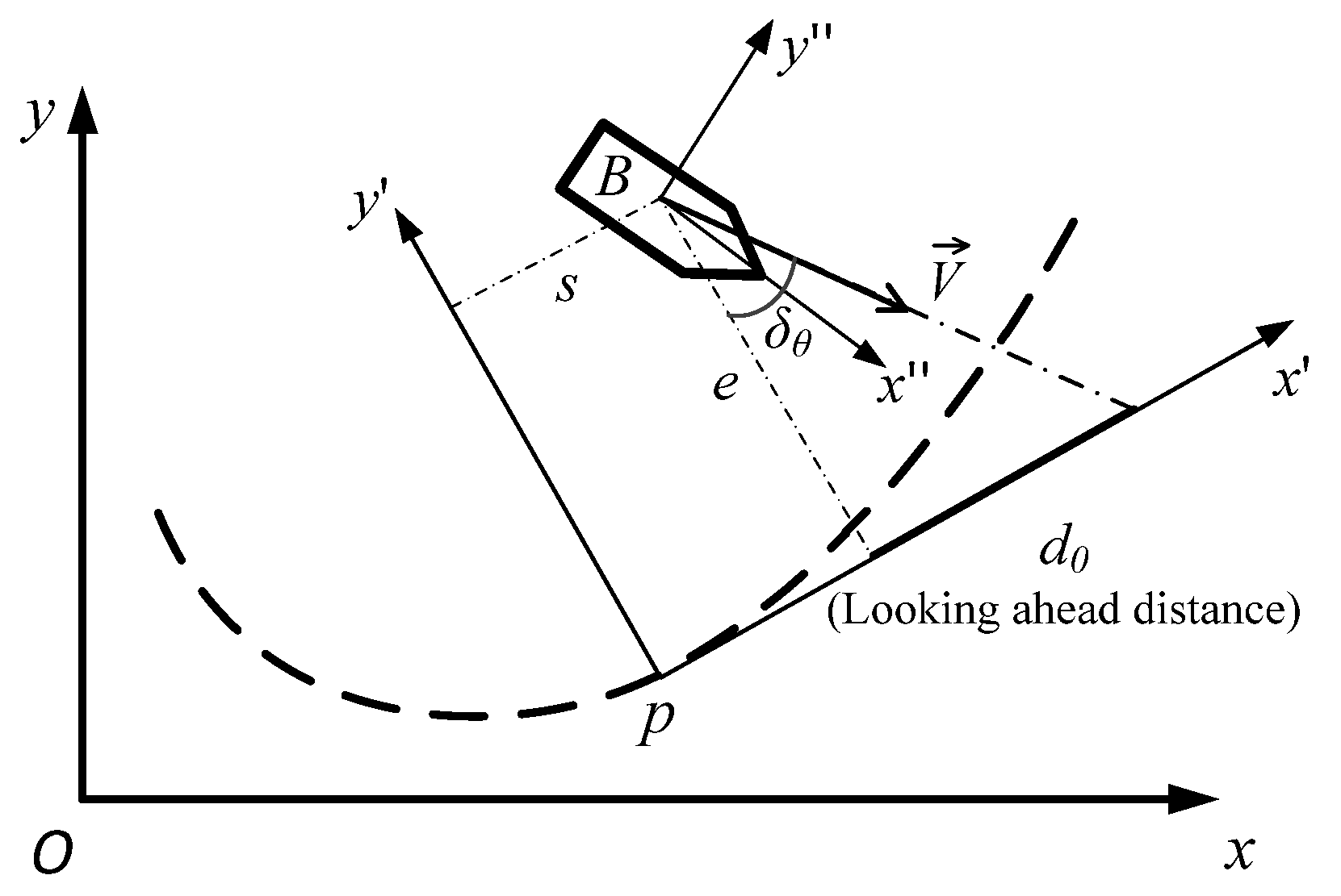
In this paper, the slow path-following subsystem is decoupled into a guidance subsystem and a control subsystem. A revised Serret–Frenet frame is adopted in the guidance subsystem to describe the ship motion in a path-fixed frame [30]. An adaptive Nomoto model is used in the control subsystem to describe the dynamics of the yaw motion in the revised Serret–Frenet frame. A time-varying parameter is introduced to capture the uncertainty of the model and is identified by the $L_1$ adaptive law. The $L_1$ adaptive control has a fast adaption speed and can deal with system uncertainties, thus is quite suitable for the path-following subsystem, which has large system uncertainties [28]. Moreover, there is a low-pass filter in the $L_1$ adaptive law which can filter the high-frequency components and give a smooth control input to the slow path-following subsystem, thus guaranteeing the input bandwidth separation.

In the roll reduction subsystem, a Proportion-Differentiation (PD) controller has a good roll reduction performance in the wave regime it is tuned for. Yet, different from the traditional separate control, where the interaction between the roll motion and the motions of other DoFs is seldom considered [21], the coupling effect is considered by introducing QSSE in this paper. In the stretched time scale τ, the coupling effect from the slow path-following subsystem in terms of rudder offsets can be regarded as a constant disturbance to the roll reduction subsystem. The coupling effect is important in the path-following problem. For example, there is a steady roll angle during the steady turning of a ship, which should be taken into the feedback law of the roll reduction control. In fact, this roll angle reflects the interaction effect of the slow path-following dynamics on the fast roll motion.

In this paper, the ship motion control problem of path-following in the horizontal plane with a simultaneous roll reduction is studied. By neglecting the heave and pitch motions in the vertical plane, a 4-DoF (surge, sway, roll, and yaw) maneuvering motion model is adopted. A comprehensive 4-DoF maneuvering motion model of a high-speed container ship [16,31] is used for the simulation study. Based on a set of captive model tests with varying heel angles, the 4-DoF equations of coupled surge–sway–roll–yaw motions are derived [31]. This maneuvering motion model is often used as the benchmark model to evaluate ship motion control performance, especially when taking the effect of roll motion into account.

The rest of the paper is structured as follows: In Section 2, a brief introduction of the singular perturbation approach used for the 4-DoF ship motion control system is given. In Section 3, the control laws for the slow and fast subsystems are designed. Section 4 shows the simulation results. The conclusions drawn from this study are presented in Section 5.

2. Time-Scale Analysis for Ship Motion System

The singular perturbation method has been used in the control industry for separating motions of different time scales since the 1960s. Nowadays, it is still widely used in the aerospace control community [32,33]. This time-scale decomposition technique was introduced to the ship motion control problem in the previous work [28]; however, the result was only limited to the RRS control in the course-keeping problem. In this paper, the RRS control in the path-following problem is addressed.

2.1. Singular Perturbation

In order to use the time-scale decomposition strategy, the real system must be modeled in the form of singular equations. Then, the standard singular perturbation procedure is to decouple the system into two subsystems: a slow subsystem with an ordinary form, and a fast subsystem, whose highest order derivatives of the state variables are multiplied by a small positive parameter ϵ [32]:

$$\dot{\mathit{x}}=\mathit{>f}\left(\mathit{x},\mathit{z},ϵ,t\right),\hspace{1em}\mathit{x}\left(t_0\right)={\mathit{x}}_0,\hspace{1em}\mathit{x}\in R^n$$

(1)

$$ϵ\dot{\mathit{z}}=\mathit{g}\left(\mathit{x},\mathit{z},ϵ,t\right),\hspace{1em}\mathit{z}\left(t_0\right)={\mathit{z}}_0,\hspace{1em}\mathit{z}\in R^m$$

(2)

where x is the slow state vector and $\mathit{z}$ represents the fast state vector; n and m denote the dimensions of the slow state vector and the fast state vector, respectively; $t_0$ is the initial time, and ${\mathit{x}}_0$ and ${\mathit{z}}_0$ are the initial state vectors. The parameter$ϵ$ ($0<ϵ\ll 1$) is a small constant, and it is usually obtained by the insight of the researchers and often has a physical meaning; for example, in a system with subsystems of different time scales, the ratio of the slow part to the fast part is often taken as ϵ, representing the difference in speed between the different subsystems. It is assumed that f and g are smooth functions. It is also assumed that the above ordinary differential equations (ODEs) have a unique solution and the system has a unique stable equilibrium.

The singular Equation (2) can be rewritten as [32]:

$$\dot{\mathit{z}}=\frac{\mathit{g}\left(\mathit{x},\mathit{z},ϵ,t\right)}{ϵ},\hspace{1em}\mathit{z}\left(t_0\right)={\mathit{z}}_0,\hspace{1em}\mathit{z}\in R^m$$

(3)

$$0=\mathit{g}\left(\overline{\mathit{x}},\overline{\mathit{z}},0,t\right)$$

(4)

Since the system has a unique equilibrium, the root of Equation (4) can be written as [32]:

$$\overline{\mathit{z}}=\mathit{h}\left(\overline{\mathit{x}},t\right)$$

(5)

where $\overline{\mathit{z}}$ is also called the QSSE of the fast dynamics. Although $\mathit{z}$ is the fast state vector, $\overline{\mathit{z}}$ is a slow state vector and represents the quasi-steady impact of the slow subsystem to the fast subsystem. To obtain the reduced-order model, the QSSE is substituted into Equation (1), while keeping the same initial condition for the state variable $\overline{\mathit{x}}\left(t\right)$ [32]:

$$\dot{\overline{\mathit{x}}}=f\left(\overline{\mathit{x}}\right),\hspace{1em}\overline{\mathit{x}}\left(t_0\right)={\mathit{x}}_0$$

(6)

This model is called the quasi-steady-state subsystem. It describes the slow dynamics of the system. Actually, Equation (6) considers the coupling effect of the fast dynamics by substituting the QSSE into Equation (1).

The essential idea of singular perturbation is to express the fast subsystem in a new time scale $\tau$, in which the slow state variables can be regarded as constants. The new time-scale is obtained by stretching the time t through dividing it by the small system constant $ϵ$ [32]:

$$\tau =\frac{t}{ϵ}$$

(7)

Under the time scale $\tau$, the fast subsystem can be expressed as [32]:

$$\frac{d\mathit{z}}{d\tau }=\mathit{g}\left(\mathit{x},\mathit{z}\left(\tau \right)\right),\hspace{1em}\tau =\frac{t}{ϵ}$$

(8)

Equation (8) is also called a boundary layer subsystem. It describes the fast dynamics in the stretched time scale $\tau$. In this time scale, x is regarded as a constant state vector and $ϵ$ defines the stretched time scale.

As long as the system is divided into the slow quasi-steady-state subsystem and the fast boundary layer subsystem, the control strategy can be designed separately in each subsystem. The control problem becomes much simpler in the reduced-order subsystems. Denoting the control inputs in the quasi-steady-state subsystem and the boundary layer subsystem as ${\sigma }_q$ and ${\sigma }_b$, respectively, the whole system control input $\sigma$ can be expressed as [32]:

$$\sigma ={\sigma }_q\left(t\right)+{\sigma }_b\left(\frac{t}{ϵ}\right)$$

(9)

However, it should be noted that the reason that the control inputs are able to be added together is the existence of bandwidth separation in the system. The bandwidth separation characteristic makes it possible that the control input in a subsystem will not severely affect the other subsystem. Fortunately, there is often a large enough bandwidth separation gap between the subsystems of different time scales when $ϵ$ is small enough. For more details about the stability issues, see [32].

2.2. Singular Perturbation Used in Ship Motion System

In this subsection, the time-scale decomposition technique for the 4-DoF ship motion system is introduced.

For simplicity, a linear model is considered in the time-domain analysis of the RRS control system, and the forward speed is assumed to be constant. The linear model of 4-DoF ship motions can be expressed in the following singular form:

$$\left\{\begin{array}{c}\dot{v}\\ \dot{\psi }\\ \dot{r}\\ ϵ\dot{\varphi }\\ ϵ\dot{p}\end{array}\right\}=\left\{\begin{array}{c}{f}_1\left(v,r,\varphi ,p,\delta \right)\\ r\\ f_2\left(v,r,\varphi ,p,\delta \right)\\ ϵp\\ ϵf_3\left(v,r,\varphi ,p,\delta \right)\end{array}\right\}$$

(10)

where $v,\psi ,r,\varphi ,p$ denote the sway speed, heading angle, yaw rate, roll angle and roll rate, respectively; $\delta$ is the rudder angle; $f_1,f_2,f_3$ are the linearized smooth functions in sway, yaw, and roll, respectively. The term $ϵ=\left(I_x+J_x\right)/\left(I_z+J_z\right)$ is defined as the small singular constant parameter, where $I_x$ and $I_z$ are the moments of inertia of the ship about the x-axis and z-axis, and $J_x$ and $J_z$ are the added moments of inertia about the x-axis and z-axis. The moment of inertia and added moment of inertia about the z-axis are usually much larger than those about the x-axis. In the present study, e.g., $\left(I_z+J_z\right)$ is taken as 41.7 times of $\left(I_x+J_x\right)$ for the ship [31]. If the roll motion equation is normalized by dividing both sides with $\left(I_z+J_z\right)$, the small parameter $ϵ$ will appear in the roll motion equation as given in Equation (10).

Following the standard time-scale decomposition procedures described above, the 4-DoF ship motion system can be decoupled into the following two subsystems:

Slow path-following subsystem:

$$\dot{\overline{v}}={\overline{a}}_{11}\overline{v}+{\overline{a}}_{12}\overline{r}+{\overline{Y}}_{\delta }\delta$$

(11)

$$\dot{\overline{\psi }}=\overline{r}$$

(12)

$$\dot{\overline{r}}={\overline{a}}_{21}\overline{v}+{\overline{a}}_{22}\overline{r}+{\overline{N}}_{\delta }\delta$$

(13)

where the bar denotes the variables that belong to the quasi-steady-state subsystem with $ϵ=0$; ${\overline{Y}}_{\delta }$and ${\overline{N}}_{\delta }$ are the derivatives with respect to the rudder angle.

Fast roll motion subsystem:

$$\frac{d\varphi }{d\tau }=g_{\varphi }\left(p\right)={\tilde{a}}_{34}p$$

(14)

$$\frac{dp}{d\tau }=g_p\left(v,r,\varphi ,p,\delta \right)={\tilde{a}}_{41}v+{\tilde{a}}_{42}r+{\tilde{a}}_{43}\varphi +{\tilde{a}}_{44}p+{\tilde{N}}_{\delta }\delta$$

(15)

where the tilde denotes the variables that belong to the stretched time-scale subsystem. The mathematical expressions of the coefficients of Equations (11)–(15) are straightforward but with very complicated forms, see [15] for more details. It should be noted that the slow-varying state variables, $v$ and $r$, actually create constant disturbances to the roll motion subsystem under the new time scale. They often cause a roll angle in the roll motion subsystem.

As long as the ship motion system is decoupled into the two subsystems of different time scales, the control laws can be designed separately for each of the reduced-order subsystems. Denoting the control laws for the path-following subsystem and the roll motion subsystem as ${\delta }_p$ and ${\delta }_r$, the total control law can be expressed as:

$$\delta ={\delta }_p\left(t\right)+{\delta }_r\left(\frac{t}{ϵ}\right)$$

(16)

A large enough bandwidth separation gap should be guaranteed in the control law design for the subsystems with different time scales, otherwise the performance of a subsystem may be interfered with by the control input of the other subsystem. The control laws for the two subsystems are discussed in the following section, especially for the slow path-following subsystem. The $L_1$ adaptive control strategy is introduced in the slow subsystem to give a smooth and effective path-following performance.

3. Control Law Design

The control law in the path-following subsystem is of great importance, because path-following performance is the primary control objective in this study and roll reduction performance can be regarded as the secondary objective. Moreover, if there is a high-frequency component of rudder command, the path-following control input may severely affect the roll reduction performance. To ensure a large enough bandwidth separation gap, the rudder input for the path-following subsystem should only consist of low-frequency components. In order to obtain a smooth and effective control input under the high frequency wave disturbances and the large system uncertainty in the path-following subsystem, the $L_1$ adaptive control is introduced to filter the high-frequency disturbances and handle the uncertainty of the system.

3.1. Slow Path-Following Subsystem

The guidance-based strategy is used in the path-following subsystem [30]. The overall structure of this path-following control strategy is shown in Figure 2. The whole path-following control system is divided into a guidance subsystem and a control subsystem. The guidance subsystem only considers the kinematic and guidance information about the system, and provides the reference heading for the ship to track. The control subsystem pays attention to the dynamics of the ship and provides the rudder command according to the $L_1$ adaptive control strategy.

3.1.1. Guidance Subsystem

Figure 3 describes the structure of the guidance-based path-following strategy. Three coordinate frames are adopted for this problem: the stationary inertial frame O, the path-fixed frame P, and the body-fixed frame B, with the origins of O, P and B, respectively. The P frame is similar to the Serret–Frenet frame [34] and is referred to as the revised Serret–Frenet frame in this paper. The origin of this frame is attached to the path, with its x′-axis pointing to the tangential direction of the path.

The bases of these three frames are expressed as ${\mathit{e}}_O=\left[e_{O1}, e_{O2}\right]$, ${\mathit{e}}_P=\left[e_{P1}, e_{P2}\right]$ and ${\mathit{e}}_B=\left[e_{B1}, e_{B2}\right]$, respectively. The relationship between these three bases can be expressed as [16]:

$${\mathit{e}}_{\alpha }={\mathit{e}}_{\beta }{\mathit{R}}_{\beta \alpha }$$

(17)

$${\mathit{R}}_{\beta \alpha }=\left(\begin{array}{cc}\cos {\theta }_{\beta \alpha }& -\sin {\theta }_{\beta \alpha }\\ \sin {\theta }_{\beta \alpha }& \cos {\theta }_{\beta \alpha }\end{array}\right)$$

(18)

where $\alpha , \beta \in$ (O, P, B), ${\theta }_{\beta \alpha }\in$ ($-\pi , \pi$); ${\theta }_{\beta \alpha }$ is the rotation angle from frame $\alpha$ to frame $\beta$, positive if they are anti-clockwise. The ${\mathit{R}}_{\beta \alpha }$ is a unit orthogonal rotation matrix between frame $\alpha$ and frame $\beta$, thus ${\mathit{R}}_{\beta \alpha }^{\mathrm{T}}={\mathit{R}}_{\beta \alpha }^{-1}={\mathit{R}}_{\alpha \beta }$.

Different from the traditional approach where the dynamic equations are described in the B frame and the kinematic equations are described in the O frame, in the guidance-based path-following strategy the equations of ship motion are all described in the revised Serret–Frenet frame P, whose origin moves along the path according to an updating law. The original tracking problem turns to a regulation problem.

In the revised Serret–Frenet frame P, the whole kinematic equations can be written as [28]:

$$\dot{s}=-{\dot{\theta }}_{PO}e+U\cos {\theta }_{WP}+V_P$$

(19)

$$\dot{e}={\dot{\theta }}_{PO}s+U\sin {\theta }_{WP}$$

(20)

$${\dot{\theta }}_{WP}=r_c$$

(21)

where s and e are the x-coordinate and y-coordinate of the vessel’s position expressed in the revised Serret–Frenet frame P; $U$ is the vessel’s total speed, and ${\theta }_{WP}$ is the angle of the vessel’s speed in the revised Serret–Frenet frame P. The term ${\theta }_{PO}$ represents the angle from the frame O to the frame P, and $r_c≔{\dot{\theta }}_{WP}$ is regarded as the input to this pure kinematic level motion. The term $V_P$ is the tangential updating speed of the frame P along the given path, also regarded as a virtual input of the system. Equations (19)–(21) are usually named error dynamics.

In the revised Serret–Frenet frame, the control objective can be set as:

$$\underset{t\to \infty }{lim}\left(\begin{array}{c}s\\ e\\ {\theta }_{WP}-{\delta }_{\theta }\end{array}\right)=\mathbf{0}$$

(22)

where:

$${\delta }_{\theta }={\sin }^{-1}\left(\frac{-e}{\sqrt{{\left|e\right|}^2+d_0^2}}\right)$$

(23)

As shown in Figure 3, ${\delta }_{\theta }$ is the desired heading angle for control output; it can be regarded as the reference angle for ${\theta }_{WP}$ to track. It is determined by the constant $d_0$, which is referred to as the looking-ahead distance. The term $d_0$ actually takes the forehead geometrical information into the control loop.

The task of control design for this guidance subsystem is to design proper control laws for $V_P$ and $r_C$, such that Equation (22) holds. The following theorem holds for the guidance subsystem [28].

Theorem 1.

The error dynamics is defined as Equations (19)–(21). If the kinematic subsystem’s inputs are set as:

$$V_P=-U\cos {\theta }_{WP}-\lambda s$$

(24)

$$r_C={\dot{\delta }}_{\theta }-k_1\left({\theta }_{WP}-{\delta }_{\theta }\right)+\frac{c_{1}eU(-\sin {\theta }_{WP}+\sin {\delta }_{\theta })}{c_2\left({\theta }_{WP}-{\delta }_{\theta }\right)}$$

(25)

where$\lambda$,$c_1$,$k_1$and$c_2$are positive constants, then the error dynamics converges to zero in domain$\Omega$:

$$\underset{t\to \infty }{lim}{\left[s\left(t\right),e\left(t\right),{\theta }_{WP}\left(t\right)-{\delta }_{\theta }\left(t\right)\right]}^T=\mathbf{0}$$

(26)

The domain$\Omega$is selected as:

$$\Omega \left(s,e,{\theta }_{WP}\right)=\{\begin{array}{c}\left|s\left(t\right)\right|\le l_0\\ \left|e\left(t\right)\right|\le l_0\\ \left|{\theta }_{WP}\right|\le \sqrt{\frac{c_1}{c_2}{l}_0^2}+sup\left({\delta }_{\theta }\left(t\right)\right)\le \frac{\pi }{2}\end{array}$$

(27)

where$l_0$is a positive constant which describes the range of the error dynamics.

This theorem shows that the guidance subsystem can be stabilized by the control input $V_P$ and $r_C$ according to Equations (24) and (25). The term $r_C$ is also regarded as a reference output for the ship to track in the control subsystem.

3.1.2. Control Subsystem

Although the traditional Nomoto model is widely used in the course-keeping problem, it is difficult to use this model to handle the path-following problem in the revised Serret–Frenet frame, because in the revised Serret–Frenet frame the parameters of the model are time-varying with the changes of position tracking states and wave disturbances. In this paper, an adaptive Nomoto model is used to describe the ship motion control subsystem. Traditionally, the heading angle $\psi$ is described in the body-fixed frame B. On the contrast, in the adaptive Nomoto model all the state variables of the ship motion control subsystem are described in the revised Serret–Frenet frame.

The form of the adaptive Nomoto model is similar to the ordinary first-order Nomoto model [34]:

$${\theta }_{WP}\left(s\right)=H\left(s\right)\delta \left(s\right)$$

(28)

$$H\left(s\right)=\frac{K_n}{\left(1+T_{n}s\right)s}$$

(29)

where ${\theta }_{WP}\left(s\right)$ and $\delta \left(s\right)$ are the Laplace transforms of ${\theta }_{WP}\left(t\right)$ and the rudder angle $\delta \left(t\right)$, respectively. The term $H\left(s\right)$ is the first-order transfer function from $\delta$ to ${\theta }_{WP}$, and $K_n$ and $T_n$ are the corresponding parameters. However, the exact values of $K_n$ and $T_n$ are not known in advance. In fact, due to different navigation situations and the time-varying environmental disturbances, the exact values of $K_n$ and $T_n$ change with time. In order to obtain an adaptive control strategy to deal with this system uncertainty, an adaptive parameter is introduced in the following control law.

To obtain an adaptive parameter to capture all the system uncertainties, Equation (28) can be rewritten in the following form:

$${\theta }_{WP}\left(s\right)=M\left(s\right)\cdot \left(\delta \left(s\right)+\sigma \left(s\right)\right)$$

(30)

where $M$(s) is a first-order reference model and $\sigma \left(s\right)$ is an adaptive parameter that captures the system uncertainty. $M$(s) and $\sigma \left(s\right)$ can be expressed as:

$$M\left(s\right)=\frac{m}{s+m},\hspace{1em}m>0$$

(31)

$$\sigma \left(s\right)=\frac{\left(H\left(s\right)-M\left(s\right)\right)\delta \left(s\right)}{M\left(s\right)}$$

(32)

where $m$ is a positive constant.

In the adaptive Nomoto control model Equation (30), the rudder angle $\delta \left(s\right)$ is regarded as the input and ${\theta }_{WP}$(s) is the output. As long as Equation (30) is obtained, the standard procedure of the $L_1$ adaptive control strategy can be divided into four steps as in [35].

• State Predictor

A time-domain state predictor equation based on Equation (30) can be obtained:

$${\dot{\widehat{\theta }}}_{WP}\left(t\right)=-m{\widehat{\theta }}_{WP}\left(t\right)+m\left(\mathsf{\delta }\left(t\right)+\widehat{\sigma }\left(t\right)\right)$$

(33)

$${\widehat{\theta }}_{WP}\left(0\right)=0$$

(34)

where the hat denotes the prediction value of the corresponding state variable. The term $\widehat{\sigma }$ is the prediction of the uniformly bounded adaptive parameter $\sigma$ defined in Equation (32), and $\widehat{\sigma }$ is governed by the following adaptive law.

• Adaptive Law

This part describes the updating strategy of the adaptive parameter $\widehat{\sigma }\left(t\right)$, which is very important in the $L_1$ adaptive control strategy. The adaptive law is mainly based on the projective operator introduced by Pomet and Praly [36], and is widely used in the control field:

$$\dot{\widehat{\sigma }}\left(t\right)={\Gamma }_C Proj\left(\widehat{\sigma }\left(t\right),-{\tilde{\theta }}_{WP}\left(t\right)\right),\hspace{1em}\widehat{\sigma }\left(0\right)=0$$

(35)

where ${\tilde{\theta }}_{WP}\left(t\right)={\widehat{\theta }}_{WP}\left(t\right)-{\theta }_{WP}\left(t\right)$ is the error signal between the system output and the state predictor. ${\Gamma }_C\in {ℛ}^{+}$ is the adaptation rate subject to a computable lower bound. The projective operator is defined as follows [36]:

$$Proj\left(p,y\right)=\{\begin{array}{l}\hspace{1em}\hspace{1em} y,\hspace{1em}\hspace{1em}\mathrm{if} ℱ\left(p\right)\le 0\\ \hspace{1em}\hspace{1em} y,\hspace{1em}\hspace{1em}\mathrm{if} ℱ\left(p\right)\ge 0 \mathrm{and} \frac{\partial ℱ\left(p\right)}{\partial p}y\le 0\\ y-\frac{ℱ\left(p\right)\frac{\partial ℱ\left(p\right)}{\partial p}y}{{\Vert \frac{\partial ℱ\left(p\right)}{\partial p}\Vert }^2}{\frac{\partial ℱ\left(p\right)}{\partial p}}^T,\hspace{1em}\hspace{1em}\mathrm{others} \end{array}$$

(36)

where:

$$ℱ\left(p\right)=\frac{2}{ℰ}\left[\sum _{i=1}^l{\left|\frac{p_i-{\rho }_i}{{\sigma }_i}\right|}^q-1+\epsilon \right]$$

(37)

$\mathrm{where} {\rho }_i \mathrm{and} {\sigma }_i \mathrm{are} \mathrm{some} \mathrm{given} \mathrm{real} \mathrm{numbers} ;$ $\epsilon$ and $q$ are real numbers, with $0<\epsilon <1$ and $q\ge 2$.

• Control Law

The adaptive control law for the path-following subsystem is selected as the difference between $r_C\left(s\right)$ and $\widehat{\sigma }\left(s\right)$ filtered by a low-pass filter:

$${\delta }_p\left(s\right)=C\left(s\right)(r_C\left(s\right)-\widehat{\sigma }\left(s\right))$$

(38)

where $C\left(s\right)$ is a first-order low-pass filter, expressed as:

$$C\left(s\right)=\frac{\omega }{s+\omega }$$

(39)

and $\omega$ is the cut-off frequency of the low-pass filter.

The control law is added with a low-pass filter, which is important in the RRS control system design, because the path-following subsystem should give a smooth rudder input to guarantee the bandwidth separation. In practice, the guidance subsystem may be disturbed by noises and provide a high-frequency reference signal $r_C$, or $\widehat{\sigma }\left(s\right)$ may have a high-frequency component at the initial time. The high-frequency components can be filtered out by the low-pass filter $C\left(s\right)$ and thus will give the slow subsystem a more appropriate control input.

• Stability Requirement

In order to have a stable control performance, there are some limitations for $C\left(s\right)$ and $M\left(s\right)$. It needs to be ensured that [35]:

$$F\left(s\right)=\frac{H\left(s\right)M\left(s\right)}{C\left(s\right)H\left(s\right)+\left(1-C\left(s\right)\right)M\left(s\right)}$$

(40)

and $F\left(s\right)$ needs to be stable to ensure the stability of the whole system. Moreover, the following relation should hold [35]:

$$\Vert G{\left(s\right)\Vert }_{L_1}{L}_z<1$$

(41)

where:

$$G\left(s\right)=F\left(s\right)\left(1-C\left(s\right)\right)$$

(42)

$$z\left(s\right)=H^{-1}\left(s\right)d\left(s\right)$$

(43)

where $d$ is the environmental disturbance; $L_z$ is the Lipschitz constant of $z\left(t\right)$ with respect to ${\theta }_{WP}\left(t\right)$. The $L_1$-norm of a single-input, single-output (SISO) system is defined as follows:

Definition 1.

The$L_1$gain of a stable and proper SISO system is defined as$\Vert N{\left(s\right)\Vert }_{L_1}={\int }_0^{\infty }\left|n\left(t\right)\right|dt$, where$n\left(t\right)$is the impulse response of$N\left(s\right)$.

If the environmental disturbances are not considered, it is easy to see that Equation (41) always holds. Otherwise, the environmental disturbance $d$ should be kept in a reasonable range to guarantee the stability of the system. The details about the stability issues can refer to [37].

3.2. Fast Roll Reduction Subsystem

The roll reduction subsystem is much simpler compared to the path-following subsystem. The roll motion subsystem Equations (14) and (15) can be rewritten as a mass-spring-damping system in the stretched time scale $\tau$:

$$\frac{d^2\varphi }{d{\tau }^2}+2\xi {\omega }_n\frac{d\varphi }{d\tau }+{\omega }_n^2\varphi =\tilde{G}\left(v,\psi ,r\right)+{\tilde{N}}_{\varphi }{\delta }_{\varphi }$$

(44)

where${\omega }_n$ is the natural frequency of roll motion and $\xi$ is the damping coefficient of the system. The term $\tilde{G}\left(v,\psi ,r\right)$ can be regarded as a constant disturbance in the time scale $\tau$, which causes a quasi-steady roll response. They and ${\tilde{N}}_{\varphi }$ are defined as:

$${\omega }_n^2=-{\tilde{a}}_{34}{\tilde{a}}_{43}$$

(45)

$$\xi =-{\tilde{a}}_{34}{\tilde{a}}_{44}/(2{\tilde{a}}_{43}\sqrt{-{\tilde{a}}_{34}{\tilde{a}}_{43}})$$

(46)

$$\tilde{G}={\tilde{a}}_{34}G\left(v,\psi ,r\right)$$

(47)

$${\tilde{N}}_{\varphi }={\tilde{a}}_{34}{\tilde{N}}_{\delta }$$

(48)

The mathematical expressions of the coefficients in Equations (45)–(48) can be found in [15].

From Equations (14) and (15), it is easy to obtain the equilibrium point of the fast subsystem:

$${\varphi }_0=\frac{G\left(v,\psi ,r\right)}{-{\tilde{a}}_{43}}$$

(49)

$$p_0=0$$

(50)

A PD controller is used to control the roll motion subsystem Equation (44):

$${\delta }_r=k_p\left(\varphi -{\varphi }_0\right)-\frac{2{\xi }_{\delta }{\omega }_n}{{\tilde{N}}_{\varphi }}\frac{d\varphi }{d\tau }$$

(51)

where $k_p$ and ${\xi }_{\delta }$ are positive constants. Substituting the control law Equation (51) into Equation (44), the total damping coefficient of the roll motion subsystem becomes ${\xi }_T=\left(\xi +{\xi }_{\delta }\right)>\xi$, thus the derived Differentiation-controller actually adds the damping to the roll motion subsystem and the Proportion-controller takes the roll angle feedback of the equilibrium point into the control system. Under such a control law, a faster decay in roll motion can be achieved.

4. Simulation Results

A nonlinear 4-DoF (surge, sway, roll, and yaw) maneuvering motion model of a single-screw, high-speed container ship [16,31] is used to evaluate the performances of the derived path-following and RRS control laws. This nonlinear model is widely used as a benchmark model in the field of ship motion control to evaluate the performances of different control strategies. The principal particulars of the ship are given in

Table 1. Principal particulars of the container ship.

Item	Symbol	Value
Overall length	L	175.0 m
Breadth	B	25.4 m
Mean draft	T	8.5 m
Displacement volume	$\nabla$	21,222 m3
Keel to transverse metacenter	KM	10.39 m
Keel to buoyancy center	KB	4.62 m
Block coefficient	CB	0.559
Rudder area	AR	33.04 m2

. More details of the nonlinear model can be found in [16].

The wave disturbances are modeled by shape functions, which are actually second-order linear approximations of the Pierson–Moskowitz spectral density functions. This kind of wave model is widely used in RRS control systems for its simplicity and validity [12,38].

Considering the wave direction, the disturbances in the path-following subsystem and the roll reduction subsystem, $w_p$ and $w_r$, can be described as:

$$w_p=h_1\left(s\right)·w\left(s\right)\cdot \sin ({\theta }_{BO}-{\theta }_0)$$

(52)

$$w_r=h_2\left(s\right)·w\left(s\right)\cdot \sin ({\theta }_{BO}-{\theta }_0)$$

(53)

where $w\left(s\right)$ is the Gaussian white noise with a variance ${\sigma }_n=0.5$ and a zero mean; ${\theta }_0$ is the wave direction. Without loss of generality, ${\theta }_0$ is assumed to be zero. The shaping filters, $h_1\left(s\right)$ and $h_2\left(s\right)$, are expressed as:

$$h_1\left(s\right)= \frac{k_{1}s}{s^2+2{\xi }_0{\omega }_{0}s+{\omega }_0^2}$$

(54)

$$h_2\left(s\right)= \frac{k_{2}s}{s^2+2{\xi }_0{\omega }_{0}s+{\omega }_0^2}$$

(55)

where $k_1$ and $k_2$ denote the dominated wave strength coefficients of yaw and roll motions. The terms ${\xi }_0$ and ${\omega }_0$ are the damping coefficient and the encountered wave frequency. Their values are selected as $k_1=1\times {10}^{-5}$,$k_2=5\times {10}^{-5}$,${\xi }_0=0.075$,${\omega }_0=0.23$, according to O’Brien [38]. These values are chosen to create a relatively large roll motion to evaluate the RRS performance; for example, ${\omega }_0$ is selected as 0.23 because it is near the ship’s natural frequency (${\omega }_n\approx 0.22$ rad/s).

A fourth-order Runge–Kutta method is used in the simulation of ship motion. The rudder saturation and rate limits ($\left|\delta \right|\le {35}^{\circ }, \left|\dot{\delta }\right|\le 5^{\circ }/\mathrm{s}$) are considered in the simulation. The total speed of the ship is around 7.2 m/s. The initial values of the state variables and ship position are selected as: $v_0=0, {\psi }_0=0, r_0=0, {\varphi }_0=0, p_0=0$ and X₀ $=$ −8000 m, and Y₀ $=$ 6000 m.

The control law parameters for the path-following subsystem are selected as: $d_0=400 \mathrm{m}$, $c_1=0.007$, $c_2=400$, $k_1=0.3$, ${\Gamma }_c=0.3$, $\lambda =10$, $m=0.2$, and $\omega =0.4$. The control law parameters for the roll reduction subsystem are selected as $k_p=0.1$ and ${\xi }_{\delta }=0.08$. The values of the control law parameters are determined by the method of trial and error, but also with some physical insight. For example, the controller gain parameter $k_p$ is tuned to have a fast response according to the roll motion subsystem Equation (44); the damping coefficient ${\xi }_{\delta }$ is tuned to have a proper damping speed to the roll motion considering the rudder constraint.

Figure 4 describes the slow path-following performances with and without $L_1$ adaptive control, both with simultaneous RRS control. The blue solid line describes the predefined path for the ship to track. There are three special points, points A, B, and C, which represent three very different turning points in the path. Point A has a relatively small curvature, point B has a medium one, and point C has a maximum curvature in the path. This path is designed as general enough to evaluate the path-following performance of the control system.

In Figure 4, the red dashed line describes the performance without the $L_1$ adaptive control. It can be seen that the control system has a relatively fast response speed, but with much larger overshoots. The control input cannot give a stable output under wave disturbances, thus there must be a lot of unnecessary rudder commands in this situation. The black solid line describes the performance with the $L_1$ adaptive control; it is shown that the trajectory is much smoother. The system turns to be stable in a short time and the control output is quite robust even with system uncertainties. There are some relatively large deviations near the point B; this is mainly caused by the geometrical complexity of the path and the large looking-ahead distance $d_0$ in this situation. The control output may have some unavoidable tracking errors due to this feedforward geometric information. However, it is necessary to have a large enough $d_0$ to guarantee the stable performance. Thus, it is necessary to make a tradeoff between the accuracy and the stability of the control system. For the RRS control in path-following problem, the stability is considered as more important than the tracking accuracy, because it is impossible to have an effective RRS performance without a stable path-following output.

Figure 5 demonstrates the performance of the error dynamics. It actually contains the same information as shown in Figure 4, but with a clearer sight of the tangential and cross-tracking errors described in the revised Serret–Frenet frame. As shown in the upper subfigure of Figure 5, the tangential error converges to zero in a very short time. It should be noted that the tangential updating law of frame P is governed by $V_P$ in Equation (24). Since the tangential error remains zero for most of the time, the revised Serret–Frenet frame is actually the same as the traditional Serret–Frenet frame. The lower subfigure of Figure 5 describes the cross errors in the cases with and without the $L_1$ adaptive control. Without the $L_1$ adaptive control, the cross error has a much larger transient overshoot and the system is not stable in a limited time. On the other hand, the performance is much better in the case with the $L_1$ adaptive control. The cross error has very small overshoots and tends to give a relatively stable cross-tracking performance, despite some small deviations.

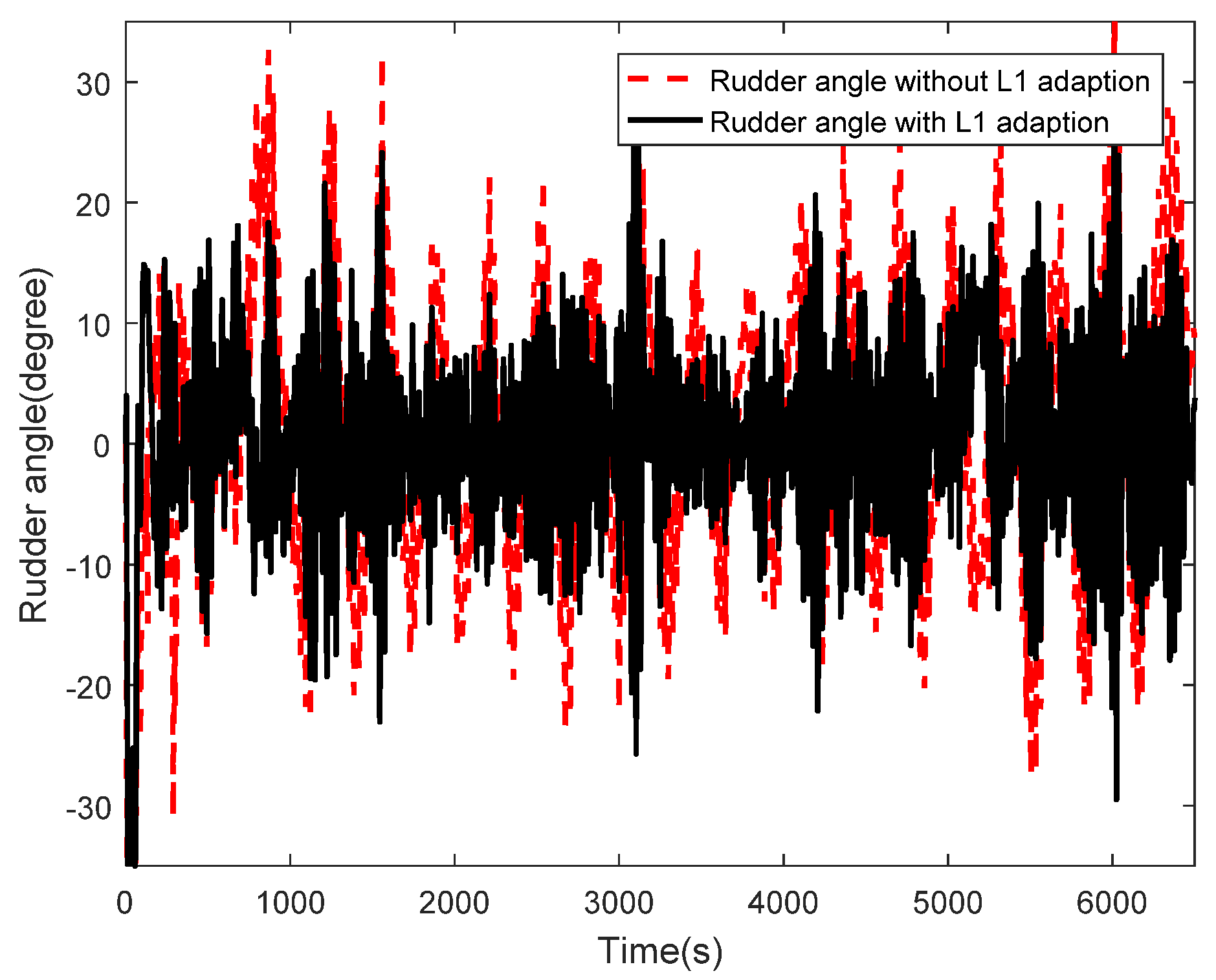
Figure 6 shows the rudder angles with and without $L_1$ adaptive control, both with RRS control at the same time. The black solid line describes the rudder angle with $L_1$ adaptive control, whose amplitude is smaller than that of the red dashed line for the rudder angle without $L_1$ adaptive control.

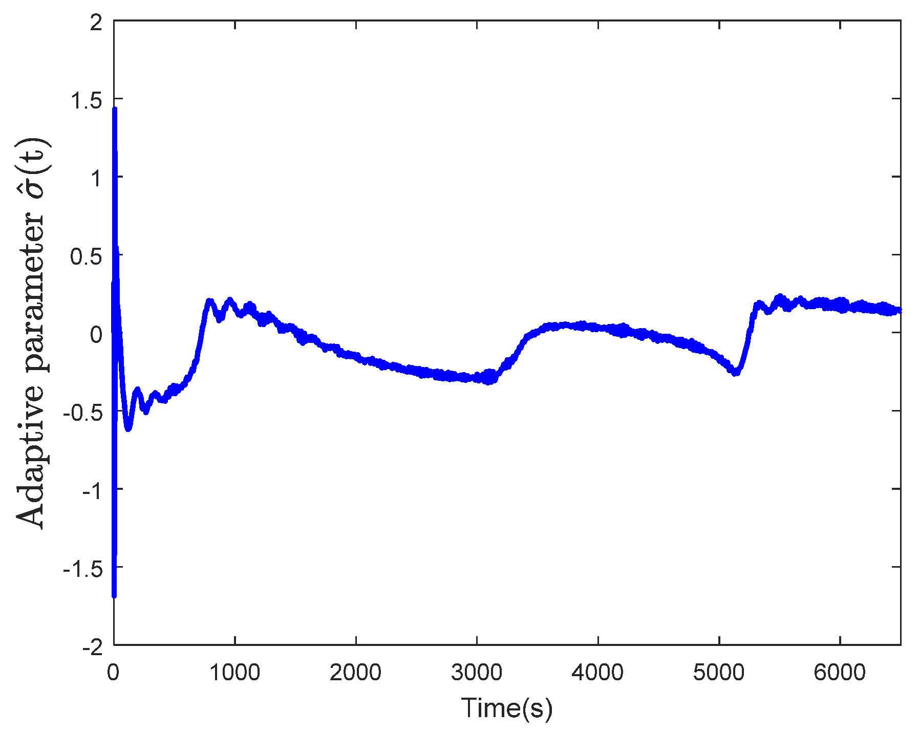
Figure 7 presents the prediction value of the adaptive parameter $\widehat{\sigma }\left(t\right)$. The value of $\widehat{\sigma }\left(t\right)$ demonstrates the uncertainty of the system and varies with the states of the system. As shown in Figure 7, the geometrical change of the path can be reflected in $\widehat{\sigma }\left(t\right)$, which has different slow-varying values at different tracking stages according to the path. The system uncertainty caused by the curve path is captured by $\widehat{\sigma }\left(t\right)$ in this way. It also shows that $\widehat{\sigma }\left(t\right)$ tends to exhibit a chattering phenomenon at the initial time and each turning point. The sudden change of the states adds large uncertainty to the system and may cause the chattering of $\widehat{\sigma }\left(t\right)$. In some sense, the chattering is inevitable in most adaptive control methods. However, the $L_1$ adaptive control has a fast adaption speed, and the value of $\widehat{\sigma }\left(t\right)$ can become stable after a very short time, which guarantees the good performance of the path-following subsystem in the long term.

.

Figure 8 shows the comparison between the desired heading angle in the guidance subsystem and the actual heading angle with the $L_1$ adaptive control. As it can be seen, both of the desired and actual heading angles can reflect the geometrical change of the path. The actual heading angle cannot track the desired heading angle for all time, since the curvature of the designed curve is large and the ship’s maneuverability is poor. However, the trends of the actual and desired heading angles are consistent; in some relatively flat parts of the path, the actual heading angle can track the desired angle with considerably high accuracy, demonstrating the good control performance. There is also a chattering phenomenon in the actual heading angle at the initial time and the sudden turning points, which is caused by the chattering of $\widehat{\sigma }\left(t\right)$ entering the feedback loop. Fortunately, the performance becomes stable after a short time.

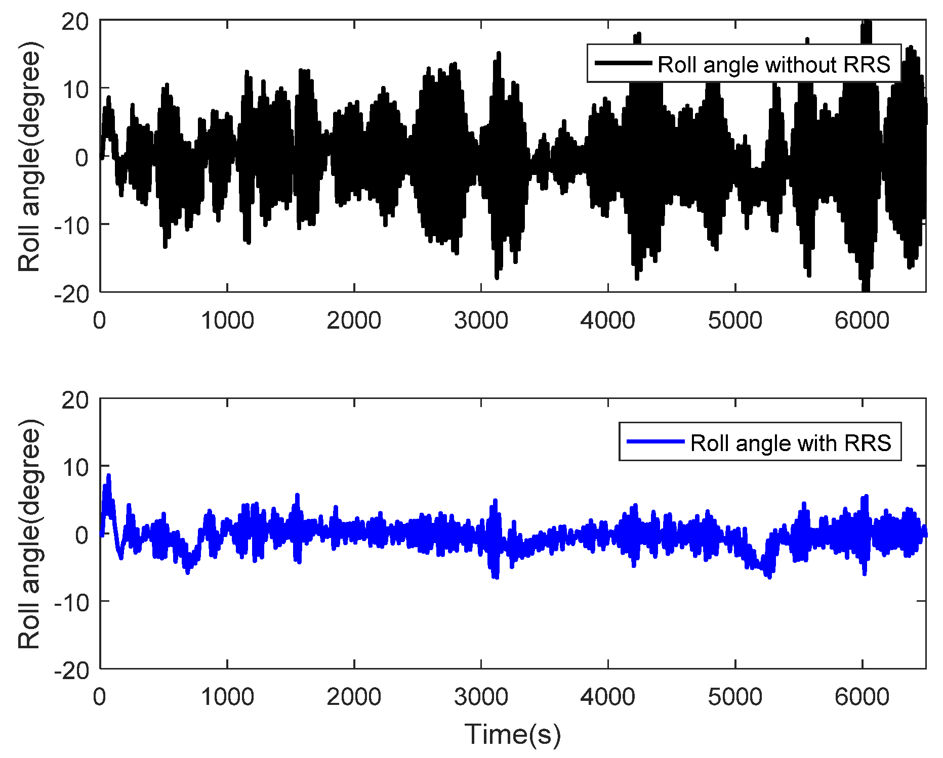
Figure 9 shows the performances of the roll reduction subsystem with and without the RRS control strategy. In these two cases, the $L_1$ adaptive control is ON in the simulation. It is easy to find out that there is a large rate of roll reduction when the subsystem has the RRS control. Without the RRS control, the roll angle is around 10° for most of the time. The peak value can reach to over 20° under the wave disturbances. However, with the RRS control the roll angle is reduced to less than 5° for most of the time. To evaluate the roll reduction performance, a so-called Roll Reduction Rate (RRR) is introduced. It is defined as [24]:

$$RRR(\%)=100\times \frac{AP-RRCS}{AP}(\%)$$

(56)

where RRCS and AP are the standard deviations with and without RRS, respectively. Under this definition, the RRR is 69.2(%) in this simulation case.

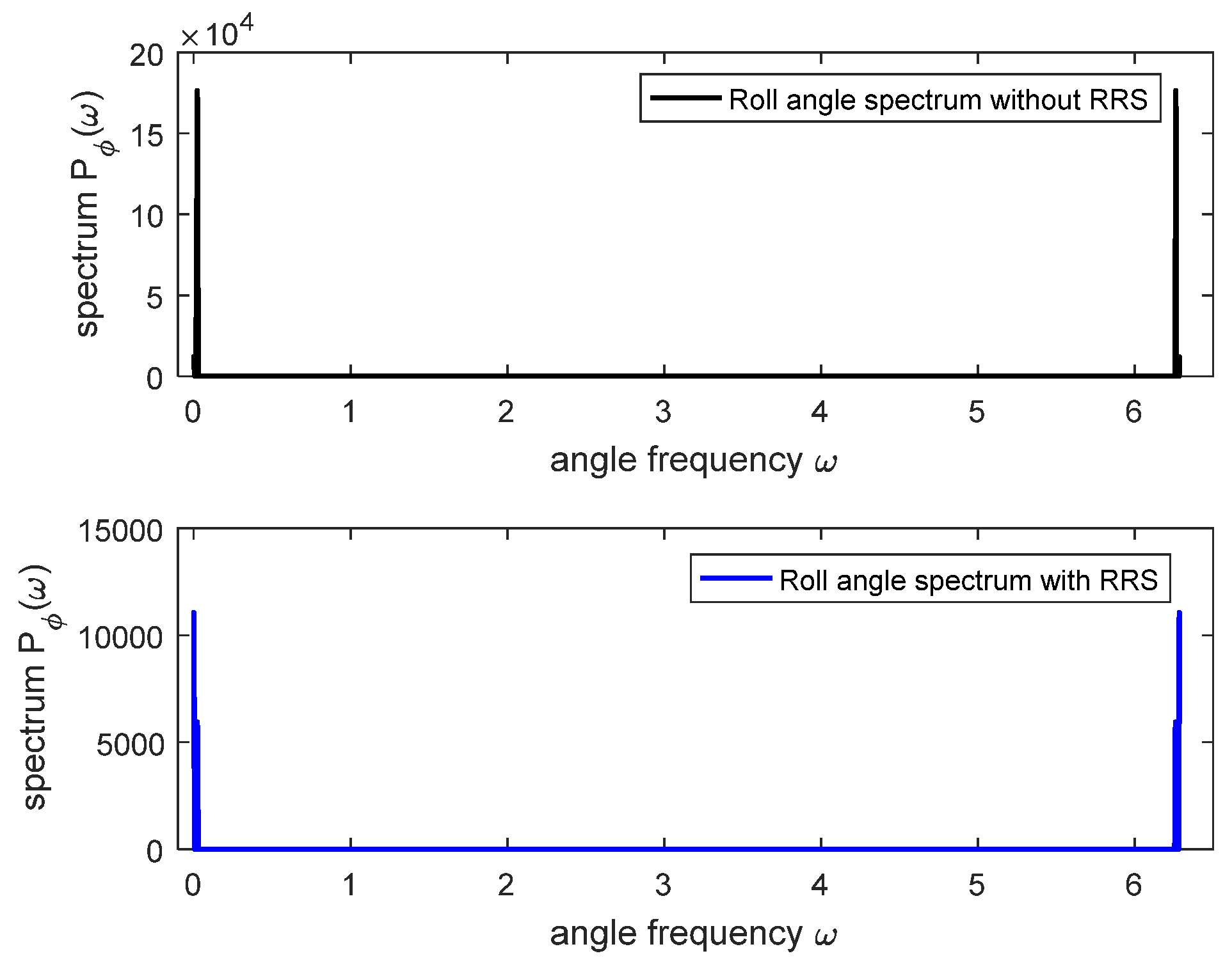
The power spectrum of the roll angle with and without RRS is presented in Figure 10. It can be seen that the amplitude without RRS is much larger than that with RRS, which validates the effectiveness of the RRS control.

Figure 11 shows the rudder commands in the slow path-following subsystem and the fast roll reduction subsystem. The rudder commands are of great importance in the time-scale analysis, because enough large input bandwidth separation gaps should be kept to guarantee the control performances of different subsystems. The upper subfigure of Figure 11 presents the rudder command in the roll reduction subsystem. It can be seen that a rudder input of a much higher frequency is needed in the roll reduction control. The lower subfigure of Figure 11 shows the rudder command in the path-following subsystem. Except for the chattering at the initial time, the rudder input is of low frequency and shows a smooth and mild change. At the turning point C, which has the maximum curvature on the path, there is a relatively large rudder command to give a sudden turning motion of the ship. It shows that there is a large enough bandwidth separation gap to guarantee that the control performance of a subsystem is not interfered with by the control input in the other subsystem. It should be noted that some rudder commands are beyond the rudder saturation and rate limits, and these commands are filtered out by the control law. Fortunately, most of the rudder commands are within the limits, which guarantees the effectiveness of the control input.

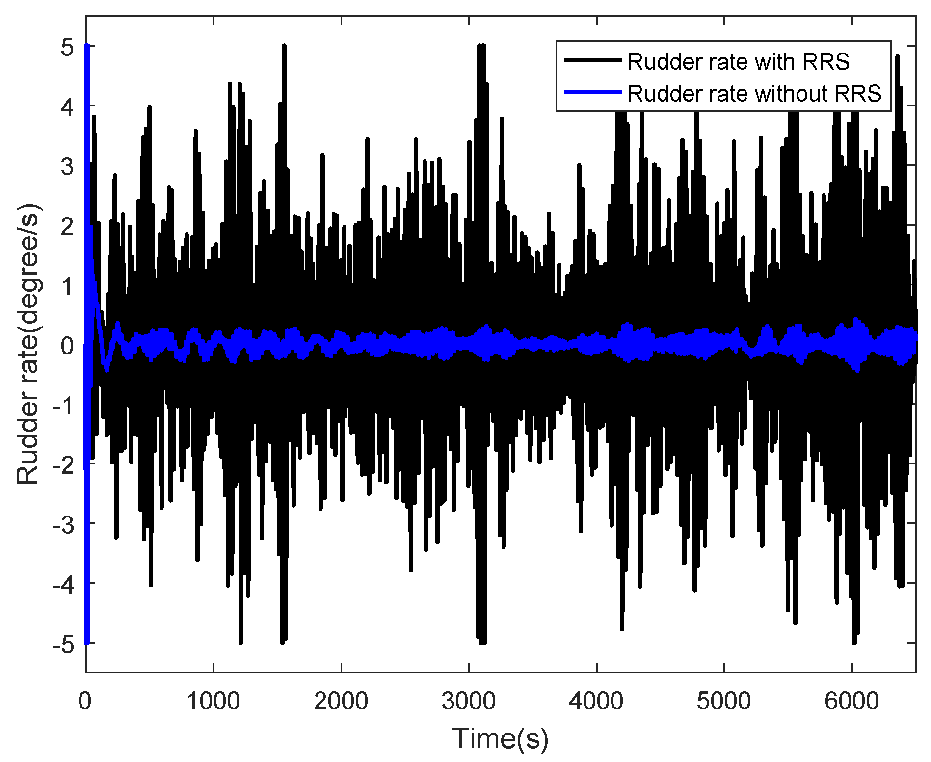
Figure 12 shows the rudder rates with and without RRS. It can be seen that the amplitude of the rudder rate with RRS is much larger than that without RRS, indicating that the good performance in roll reduction is at the expense of rapid steering.

To demonstrate whether the RRS control in the fast subsystem affects the path-following performance, a comparison of the path-following performances with and without the RRS control is conducted. The results are presented in Figure 13, where the black solid line is the performance with RRS control and the red dashed line is the performance without RRS control. It can be seen that they almost overlap with each other, indicating that the RRS control has very little influence on the path-following performance.

Figure 14 demonstrates the influence of the $L_1$ adaptive control strategy on the roll reduction performance. It shows that the roll reduction performance is apparently affected by the $L_1$ adaptive control. The roll angles are a little smaller when the adaptive control is ON, and the performance curve without adaptive control is more periodic than that with adaptive control. This is mainly due to the fact that the control performances of the slow path-following subsystem in these two cases are very different. Without the $L_1$ adaptive control, there exists a periodic overshooting as shown in Figure 4, which results in the quasi-periodic properties of the roll motion as shown in the upper subfigure of Figure 14. While in the case with the $L_1$ adaptive control, the path-following performance is more stable and milder, and thus has a very limited interference to the roll reduction subsystem. It shows that the path-following performance may greatly affect the roll reduction performance. Thus, it is desirable to pay more attention to the control design of the slow path-following subsystem. Fortunately, the $L_1$ adaptive control can help to reduce the roll motion to some extent.

5. Conclusions

In this paper, the time-scale decomposition techniques based on the singular perturbation method are used to separate the 4-DoF ship motion system into two subsystems of different time scales: the slow path-following subsystem and the fast roll reduction subsystem. The path-following performance and the rudder roll stabilization (RRS) performance are the two control objectives, with the former as the primary control objective and the latter as the secondary one. The control laws for the two subsystems are designed separately, with the coupling effects between the subsystems being taken into account. To guarantee a large enough input bandwidth separation gap, the $L_1$adaptive control is adopted in the path-following subsystem to give a robust, stable and adaptive control performance. A PD controller is used in the roll reduction subsystem.

A widely used nonlinear 4-DoF maneuvering motion model of a container ship is adopted for the simulation study. The results show that in the slow subsystem, the path-following performance is much better when the $L_1$ adaptive control is in use. The adaptive parameter can successfully capture the system uncertainty and provide a fast adaption speed. Most importantly, the $L_1$ adaptive control strategy gives a low-frequency control input in the path-following subsystem under the wave disturbances, thus guarantees the input bandwidth separation. In the fast subsystem, the Roll Reduction Rate (RRR) can reach about 70%. The mutual interference effects of the two subsystems are also evaluated. It shows that the RRS control has very little interference in the path-following control. On the other hand, the $L_1$ adaptive control has some positive influence on the roll reduction performance.

However, it should be noted that in the present study, the effects of the heave and pitch motions in the vertical plane are neglected in the analysis and control law design. In reality, a ship sailing in waves will definitely have 6-DoF oscillating motions including heave and pitch motions. Although the present study focuses on the control problem of path-following in the horizontal plane with roll reduction at the same time, for a more practical application, it is desirable to clarify in a further study the extent to which the control performances are affected by the heave and pitch motions by using a 6-DoF maneuvering motion model for simulation study.

Moreover, the RRS control may face the issue of the overuse of steering gear if the proposed control strategy is implemented on a real ship, and the rudder rate is relatively much larger than that in the traditional course-keeping problem, which will cause the rudder to be more vulnerable to damage. Therefore, it should be used only in some emergency situations, such as when the ship encounters severe wave disturbances which may cause dangerous roll motions. In the future, a study on the factor of steering gear and the stability analysis should be conducted to create a better tradeoff between the roll reduction and operation of the steering gear when using the RRS control strategy.

References

1. Treakle, T.W.; Mook, D.T.; Liapis, S.I.; Nayfeh, A.H. A time-domain method to evaluate the use of moving weights to reduce the roll motion of a ship. Ocean Eng. 2000, 27, 1321–1343. [Google Scholar] [CrossRef]
2. Gawad, A.F.A.; Ragab, S.A.; Nayfeh, A.H.; Mook, D.T. Roll stabilization by anti-roll passive tanks. Ocean Eng. 2001, 28, 457–469. [Google Scholar] [CrossRef]
3. Perez, T.; Blanke, M. Simulation of Ship Motion in Seaway; Tech. Rep. EE02037; Department of Electrical and Computer Engineering, The University of Newcastle: Newcastle, NSW, Australia, 2002. [Google Scholar]
4. Townsend, N.C.; Murphy, A.J.; Shenoi, R.A. A new active gyrostabilizer system for ride control of marine vehicles. Ocean Eng. 2007, 34, 1607–1617. [Google Scholar] [CrossRef]
5. Surendran, S.; Lee, S.K.; Kim, S.Y. Studies on an algorithm to control the roll motion using active fins. Ocean Eng. 2007, 34, 542–551. [Google Scholar] [CrossRef]
6. Källström, C.G. Control of yaw and roll by rudder/fin stabilization system. In Proceedings of the 6th International Ship Control Systems Symposium, Ottawa, ON, Canada, 26–30 October 1981. [Google Scholar]
7. Van der Klugt, P.G.M. Rudder Roll Stabilization. Ph.D. Thesis, Delft University of Technology, Delft, The Netherlands, 1987. [Google Scholar]
8. Källström, C.G.; Wessel, P.; Sjölander, S. Roll reduction by rudder control. In Proceedings of the 13th STAR (Ship Technology and Research) Symposium, Pittsburgh, PA, USA, 8–10 June 1988. [Google Scholar]
9. Blanke, M.; Haals, P.; Andreasen, K.K. Rudder roll damping experience in Denmark. In Proceedings of the IFAC Workshop on Control Applications in Marine Systems, CAMS’89, Lyngby, Denmark, 28–30 August 1989. [Google Scholar]
10. Van Amerongen, J.; Van der Klugt, P.G.M.; Van Nauta Lemke, H.R. Rudder roll stabilization for ships. Automatica 1990, 26, 679–690. [Google Scholar] [CrossRef]
11. Blanke, M.; Christensen, A.C.S. Rudder-roll damping autopilot robustness to sway-yaw-roll couplings. In Proceedings of the 10th Ship Control Systems Symposium, Ottawa, ON, Canada, 25–29 October 1993. [Google Scholar]
12. Lauvdal, T.; Fossen, T.I. Rudder roll stabilization of ships subject to input rate saturation using a gain scheduled control law. In Proceedings of the IFAC Conference on Control Applications in Marine Systems, CAMS’98, Fukuoka, Japan, 27–30 October 1998; IFAC Proceedings Volumes. Volume 31, pp. 111–116. [Google Scholar] [CrossRef]
13. Perez, T. Control System Design for Autopilots with Rudder Roll Stabilisation. In Ship Motion Control: Course Keeping and Roll Stabilisation Using Rudder and Fins; Springer: London, UK, 2005. [Google Scholar] [CrossRef]
14. Perez, T.; Blanke, M. Ship roll damping control. Annu. Rev. Control 2012, 36, 129–147. [Google Scholar] [CrossRef] [Green Version]
15. Ren, R.Y.; Zou, Z.J.; Wang, X.G. A two-time scale control law based on singular perturbations used in rudder roll stabilization of ships. Ocean Eng. 2014, 88, 488–498. [Google Scholar] [CrossRef]
16. Fossen, T.I. Guidance and Control of Ocean Vehicles; John Wiley & Sons: New York, NY, USA, 1994. [Google Scholar]
17. Cowley, W.; Lambert, T. Sea trials on a roll stabilizer using the ship’s rudder. In Proceedings of the 4th Ship Control Systems Symposium, The Hague, The Netherlands, 27–31 October 1975. [Google Scholar]
18. Blanke, M.; Adrian, J.; Larsen, K.E.; Bentsen, J. Rudder roll damping in coastal region sea conditions. In Proceedings of the 5th IFAC Conference on Manoeuvring and Control of Marine Craft, Aalborg, Denmark, 23–25 August 2000; IFAC Proceedings Volumes. Volume 33, pp. 39–44. [Google Scholar] [CrossRef]
19. Grimble, M.J.; Katebi, M.R.; Zhang, Y. H∞-based ship fin-rudder roll stabilization design. In Proceedings of the 10th Ship Control Systems Symposium, Ottawa, ON, Canada, 25–29 October 1993. [Google Scholar]
20. Crossland, P. The effect of roll-stabilisation controllers on warship operational performance. Control Eng. Pract. 2003, 11, 423–431. [Google Scholar] [CrossRef]
21. Fang, M.C.; Luo, J.H. On the track keeping and roll reduction of the ship in random waves using different sliding mode controllers. Ocean Eng. 2007, 34, 479–488. [Google Scholar] [CrossRef]
22. Li, Z.; Sun, J.; Oh, S. Path following for marine surface vessels with rudder and roll constraints: An MPC approach. In Proceedings of the 2009 American Control Conference, St. Louis, MO, USA, 10–12 June 2009. [Google Scholar] [CrossRef]
23. Liu, C.; Sun, J.; Zou, Z.J. Integrated Line of Sight and Model Predictive Control for path following and roll motion control using rudder. J. Ship Res. 2015, 59, 99–112. [Google Scholar] [CrossRef]
24. Lauvdal, T.; Fossen, T.I. Nonlinear rudder-roll damping of non-minimum phase ships using sliding mode control. In Proceedings of the 1997 European Control Conference, Brussels, Belgium, 1–4 July 1997. [Google Scholar]
25. Stoustrup, J.; Niemann, H.H.; Blanke, M. Roll damping by rudder control—A new H∞ approach. In Proceedings of the 3rd IEEE Conference on Control Applications, Glasgow, UK, 24–26 August 1994. [Google Scholar] [CrossRef]
26. Cao, C.; Hovakimyan, N. Design and analysis of a novel L1 adaptive controller, Part 1: Control signal and asymptotic stability. In Proceedings of the 2006 American Control Conference, Minneapolis, MN, USA, 14–16 June 2006. [Google Scholar] [CrossRef]
27. Breu, D.A.; Fossen, T.I. L1 adaptive and extremum seeking control applied to roll parametric resonance in ships. In Proceedings of the 9th IEEE International Conference on Control and Automation, Santiago, Chile, 19–21 December 2011. [Google Scholar] [CrossRef]
28. Ren, R.Y.; Zou, Z.J.; Wang, X.G. L1 adaptive control used in path following of surface ships. In Proceedings of the 33rd Chinese Control Conference, Nanjing, China, 28–30 July 2014. [Google Scholar] [CrossRef]
29. Sørensen, M.E.N.; Breivik, M. Comparing nonlinear adaptive motion controllers for marine surface vessels. In Proceedings of the 10th IFAC Conference on Manoeuvring and Control of Marine Craft, Copenhagen, Denmark, 24–26 August 2015. [Google Scholar] [CrossRef]
30. Breivik, M.; Fossen, T.I. Guidance-based path following for autonomous underwater vehicles. In Proceedings of the OCEANS 2005 MTS/IEEE, Washington, DC, USA, 18–23 September 2005. [Google Scholar] [CrossRef]
31. Son, K.H.; Nomoto, K. On the coupled motion of steering and rolling of a high-speed container ship. Nav. Arch. Ocean Eng. 1982, 20, 73–83. [Google Scholar] [CrossRef]
32. Kokotovic, P.; Khalil, H.K.; O’Reilly, J. Singular Perturbation Methods in Control: Analysis and Design; Academic Press: London, UK, 1986. [Google Scholar] [CrossRef] [Green Version]
33. Esteban, S.; Gordillo, F.; Aracil, J. Three-time scale singular perturbation control and stability analysis for an autonomous helicopter on a platform. Int. J. Robust Nonlin. 2013, 23, 1360–1392. [Google Scholar] [CrossRef]
34. Fossen, T.I. Handbook of Marine Craft Hydrodynamics and Motion Control; John Wiley & Sons: New York, NY, USA, 2011. [Google Scholar] [CrossRef]
35. Kaminer, I.; Yakimenko, O.; Dobrokhodov, V.; Pascoal, A.; Hovakimyan, N.; Cao, C.; Young, A.; Patel, V. Coordinated path following for time-critical missions of multiple UAVs via L1 adaptive output feedback controllers. In Proceedings of the AIAA Guidance, Navigation and Control Conference and Exhibit, Hilton Head, SC, USA, 20–23 August 2007. [Google Scholar] [CrossRef] [Green Version]
36. Pomet, J.B.; Praly, L. Adaptive nonlinear regulation: Estimation from the Lyapunov equation. IEEE Trans. Automat. Contr. 1992, 37, 729–740. [Google Scholar] [CrossRef] [Green Version]
37. Cao, C.; Hovakimyan, N. Guaranteed transient performance with L1 adaptive controller for systems with unknown time-varying parameters and bounded disturbances: Part I. In Proceedings of the 2007 American Control Conference, New York, NY, USA, 9–13 July 2007. [Google Scholar] [CrossRef]
38. O’Brien, J.F. Multi-path nonlinear dynamic compensation for rudder roll stabilization. Control Eng. Pract. 2009, 17, 1405–1414. [Google Scholar] [CrossRef]
Figure 1. Overall scheme of the time-scale analysis for the control system of 4-DoF ship motion.
Jmse 09 01024 g001
Figure 2. Path-following control strategy.
Jmse 09 01024 g002
Figure 3. Guidance-based path-following scheme.
Jmse 09 01024 g003
Figure 4. Path-following performances with and without the L 1 adaptive control.
Jmse 09 01024 g004
Figure 5. Tangential and cross errors with and without L 1 adaptive control.
Jmse 09 01024 g005
Figure 6. Rudder angles with and without the L 1 adaptive control.
Jmse 09 01024 g006
Figure 7. Adaptive parameter σ ^ ( t ) .
Jmse 09 01024 g007
Figure 8. Desired heading angle and actual heading angle.
Jmse 09 01024 g008
Figure 9. Roll reduction performance with and without RRS.
Jmse 09 01024 g009
Figure 10. Power spectrum of roll angle with and without RRS.
Jmse 09 01024 g010
Figure 11. Rudder commands in the slow subsystem and the fast subsystem.
Jmse 09 01024 g011
Figure 12. Rudder rate with and without RRS.
Jmse 09 01024 g012
Figure 13. Path-following performances with and without RRS control.
Jmse 09 01024 g013
Figure 14. Roll reduction performances with and without L 1 adaptive control.
Jmse 09 01024 g014