Real-Time Management of Vessel Carbon Dioxide Emissions Based on Automatic Identification System Database Using Deep Learning

Abstract

In this study, we propose an effective method using deep learning to strengthen real-time vessel carbon dioxide emission management. We propose a method to predict real-time carbon dioxide emissions of the vessel in three steps: (1) convert the trajectory data of the fixed time interval into a spatial–temporal sequence, (2) apply a long short-term memory (LSTM) model to predict the future trajectory and vessel status data of the vessel, and (3) predict the carbon dioxide emissions. Automatic identification system (AIS) database of a liquefied natural gas (LNG) vessel were selected as the sample and we reconstructed the trajectory data with a fixed time interval using cubic spline interpolation. Applying the interpolated AIS data, the carbon dioxide emissions of the vessel were calculated based on the International Towing Tank Conference (ITTC) recommended procedures. The experimental results are twofold. First, it reveals that vessel emissions are currently underestimated. This study clearly indicates that the actual carbon dioxide emissions are higher than those reported. The finding offers insight into how to accurately measure the emissions of vessels, and hence, better execute a greenhouse gases (GHGs) reduction strategy. Second, the LSTM model has a better trajectory prediction performance than the recurrent neural network (RNN) model. The errors of the trajectory endpoint and carbon dioxide emissions were small, which shows that the LSTM model is suitable for spatial–temporal data prediction with excellent performance. Therefore, this study offers insights to strengthen the real-time management and control of vessel greenhouse gas emissions and handle those in a more efficient way.

1. Introduction

1.1. Greenhouse Gases (GHGs) of Vessels

With global warming progressing worldwide, each government’s emission management for greenhouse gases (GHGs) is becoming more meticulous. GHG emissions from vessels are receiving increasing attention, especially in port cities, since vessels have become a major source of polluting emissions. Most governments have introduced emission tax rates to reduce the GHG emissions of vessels, especially emissions of carbon dioxide (CO₂), which is one of the most important greenhouse gases.

Since automatic identification system (AIS) database store the detailed real-time trajectory data of vessels, we can use longitude, latitude, speed over ground (SOG) and course over ground (COG) to accurately, and in real-time, estimate the carbon dioxide emissions while the vessel is sailing. Many studies have been carried out to estimate vessel inventories using AIS data. Mabunda et al. [1] estimated a ship emission inventory near the strait of Gibraltar. Winther et al. [2] implemented emission inventory estimation in the Arctic though a S-AIS (satellite automatic identification system). The International Maritime Organization [3] implemented full-scale vessel emission inventory analysis using AIS data. Coello et al. [4] estimated an emission inventory from a UK fishing fleet, and Yao et al. [5] estimated vessel emission inventories in an estuary of the Yangtze River. Wang et al. [6] used the Ship Traffic Emissions Assessment Model (STEAM2) to estimate the fuel consumption of a vessel, though wave and wind resistance were not considered and the average speed had insufficient accuracy. Kim et al. [7] considered that the accuracy of the calculation could be improved by solving the problem of an unstable AIS data interval.

1.2. Vessel Trajectory Prediction in Deep Learning

Generally, vessel trajectory data can be represented as a set of multi-dimensional spatial–temporal sequences {($p_1,a_1,t_1$), ($p_2,a_2,t_2$), ($p_3, a_3,t_3$),…, ($p_n,a_n,t_n$)}, where $p_i$ is the position (longitude, latitude), $a_i$ is the data attribute (SOG, COG) and $t_i$ is the recording time of the AIS data.

Traditional trajectory prediction methods are linear prediction methods, but linear methods have limitations when it comes to constructing the kinematics equations of the vessel. Some traditional methods apply Gaussian-based models. Laxhammar et al. [8] proposed a Gaussian mixture model that combines multiple probability distributions to model vessel trajectories. Its disadvantage, however, was in determining the number and quantity of Gaussian components; few Gaussian components made it difficult to describe the vessel’s trajectory, and too many were prone to overfitting. Zhao et al. [9] proposed an improved Kalman filter algorithm with system noise estimation to predict the vessel’s trajectory; however, this method of setting parameters was complicated and difficult to reproduce. In addition, the marine environment had a great influence on the trajectory of vessels, which made research difficult.

Considering the inefficiency of linear relationships for different spatial–temporal data, as discussed in previous studies, we opted to use the neural network method to fit the relationship between the historical trajectory data and the next-time data. Deep learning is an algorithm that uses artificial neural networks as a framework to perform characterization learning on data. It can automatically learn the information in the data, and can learn the essential characteristics of the dataset. As a subset of machine learning methods, deep learning automatically extracts data features, which reduces the manual extraction workload and improves prediction efficiency.

Some scholars have applied deep learning to AIS data prediction. Quan et al. [10] established the recurrent neural network-long short-term memory (RNN-LSTM) model to predict vessel trajectory. Nguyen et al. [11] used the sequence-to-sequence model to predict vessel trajectory, while the encoder and decoder used long short-term memory (LSTM). However, the vessel trajectory data were spatial–temporal sequence data that had both temporal and spatial correlation. The SOG of the vessel will affect the distance the vessel travels, and the COG of the vessel will affect the position of the vessel. Therefore, some scholars proposed using the convolutional layer to extract the spatial characteristics of the trajectory data, and then used the LSTM model to analyze the temporal characteristics. This also achieved precise prediction results. For example, Ljunggren et al. [12] used convolutional networks of different sizes to learn spatial–temporal sequences in trajectory features, separate the different features in the data and finally, synthesize a feature to perform trajectory prediction. Wang and Liu [13] proposed a convolutional neural network model combined with LSTM, studying the spatial structure and temporal characteristics of vessel trajectory data simultaneously; the prediction effect was better than using the convolutional neural network alone, but the prediction error was not overwhelming compared to the LSTM model. There are also studies that examine the accuracy of machine learning methodologies on real datasets in vessels [14,15].

Existing studies suggest that the LSTM model is a suitable algorithm for vessel trajectory prediction applications. However, studies predicting emissions applying reconstructed trajectory data in deep-learning models have been scarce. This study aims to fill the research gap.

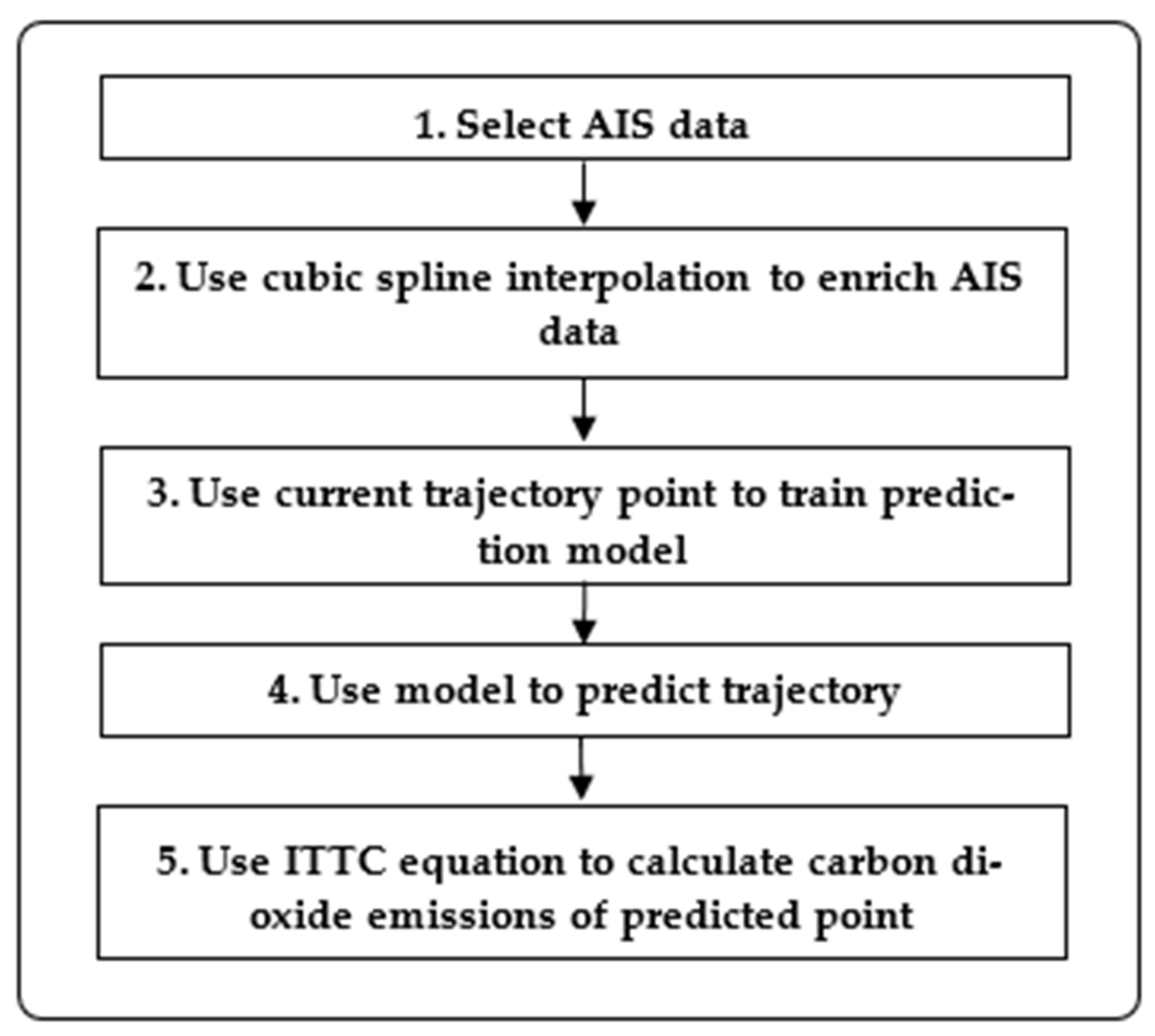
1.3. The Motivation of the Study

The motivation of this study is to strengthen the real-time management of vessel carbon dioxide emissions and to control vessel GHG emissions in a more efficient way. To achieve that, we propose a method that can accurately grasp the current emissions of the ship and predict the future emissions status. We consider that the incompleteness of the AIS trajectory data will affect the accuracy of the vessel carbon dioxide emissions estimation. As such, we propose using the cubic spline interpolation method to enrich the vessel trajectory. With this method, we can estimate the vessel carbon dioxide emissions every 1 s to improve the estimation accuracy. Thereafter, we use the LSTM model to learn the historical SOG characteristics and trajectory characteristics of vessels, to predict the spatial–temporal distribution of vessels’ future carbon dioxide emissions.

Deep learning can learn the basic characteristics of the data from a small number of samples through a deep non-linear network structure, which is suitable for rapid analysis of vessel data in the marine environment, so we chose deep learning. To improve the validity of the prediction data, we emphasized a real-time and short-term nature. Figure 1 outlines the flow of this study.

The rest of the paper is structured as follows. Section 2 describes the formation of the cubic spline interpolation model for reconstructing trajectory data, the LSTM model for prediction and the CO₂ emission estimation model. Section 3 discusses the experiments and results. Section 4 summarizes the work and the prospects for future studies.

2. Equations of the Model

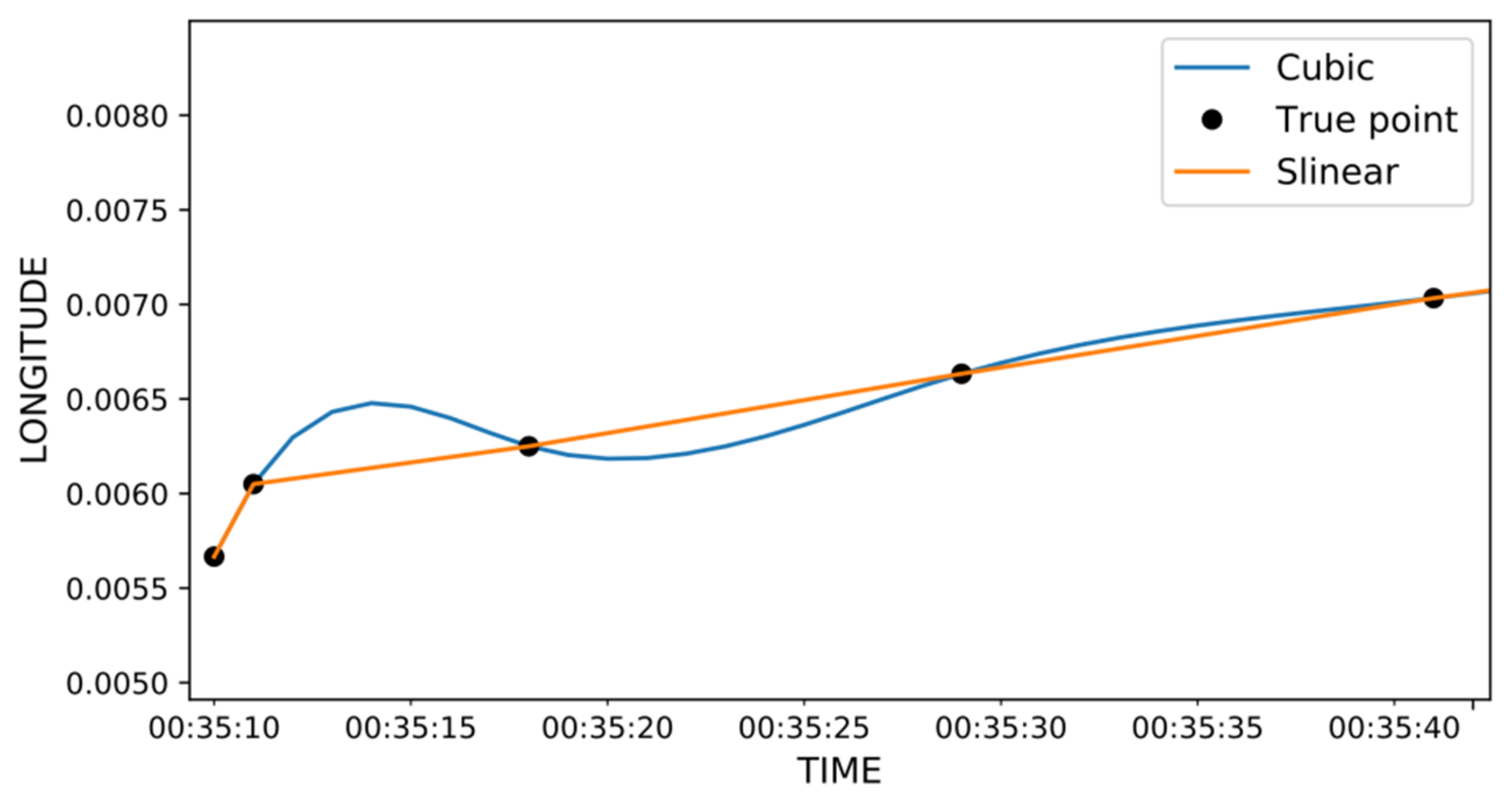
2.1. Cubic Spline Interpolation Model

Due to incorrect operation of the AIS system by shore and vessel personnel, information transmission failure between AIS and the shore base, subjective and objective factors such as the random failure of the AIS system itself or the problem of artificial improper maintenance, we need to select a method of interpolation and repair the trajectory to obtain more accurate and complete vessel trajectory information. Compared with the linear interpolation model, the non-linear interpolation model is more in line with the actual sailing state of the ship; especially near the coast, the ship cannot always keep a straight line sailing, but will adjust the course according to different sea conditions. Therefore, we select the method of cubic spline interpolation to smooth the vessel trajectory.

We suppose that the interval of trajectory data is [a, b], divided [a, b] into n intervals, as [($x_0, x_1$), ($x_1, x_2$), $\cdots$, ($x_{n-1}, x_n$)], $x_0=a, x_n=b$, where the function expression for each interval is S(x). Cubic spline means that the curve of each interval is a cubic equation $S_i\left(x\right)$ that meets the interpolation conditions $S\left(x_i\right)=y_i$ and meets the condition of a smooth curve where $S_i\left(x\right)$, $S_i{}^{\prime }\left(x\right)$, ${S_i}^{″}\left(x\right)$ are a continuous function. The solved equation (Bartels et al. [16]) is as follows:

$$S_i\left(x\right)=a_i+b_i\left(x-x_i\right)+c_i{\left(x-x_i\right)}^2+d_i{\left(x-x_i\right)}^3$$

(1)

$${S_i}^{\prime }\left(x\right)=b_i+2c_i\left(x-x_i\right)+3d_i{\left(x-x_i\right)}^2$$

(2)

$${S_i}^{″}\left(x\right)=2c_i+6d_i\left(x-x_i\right)$$

(3)

where $S_i\left(x\right)$ is the cubic spline model expression, and $a_i,b_i,c_i,d_i$ are the parameters to be solved.

Accordingly, $S_i\left(x\right)$ must meet interpolation conditions $S\left(x_i\right)=y_i$ and Equations (1)–(3). Then, we can obtain the equation as follows:

$$a_i=y_i$$

(4)

$$h_i=x_{i+1}-x_i$$

(5)

$$a_i+b_i{h}_i+c_i{h}_i{}^2+d_i{h}_i{}^3=y_{i+1}$$

(6)

According to continuous function conditions,

$$S_i^{″}\left(x_{i+1}\right)=S_{i+1}^{″}\left(x_{i+1}\right)$$

(7)

$$S_i^{‴}\left(x_{i+1}\right)=S_{i+1}^{‴}\left(x_{i+1}\right)$$

(8)

We can obtain the equation as follows:

$$b_i+2h_i{c}_i+3h_i^2{d}_i=b_{i+1}$$

(9)

$$2c_i+6h_i{d}_i=2c_{i+1}$$

(10)

$$d_i=\frac{m_{i+1}-m_i}{6h_i}\left(m_i=2c_i\right)$$

(11)

Inputting Equations (4), (10) and (11) into Equation (6), we can obtain the equation as follows:

$$b_i=\frac{y_{i+1}-y_i}{h_i}-\frac{h_i}{2}{m}_i-\frac{h_i}{6}\left(m_{i+1}-m_i\right)$$

(12)

By inputting Equations (4) and (10)–(12) into Equation (9), we can obtain the equation as follows:

$$h_i{m}_i+2\left(h_i+h_{i+1}\right)m_{i+1}+h_{i+1}{m}_{i+2}=6\left[\frac{y_{i+2}-y_{i+1}}{h_{i+1}}-\frac{y_{i+1}-y_i}{h_i}\right]$$

(13)

We build linear equations with $m$ as the unknown ($m_0=0, m_n=0$):

$$\left[\begin{array}{cccccc}1& 0& 0& 0& \cdots & 0\\ h_0& 2\left(h_0+h_1\right)& h_1& 0& \cdots & 0\\ 0& h_1& 2\left(h_1+h_2\right)& h_2& \cdots & 0\\ 0& 0& h_2& 2\left(h_1+h_2\right)& h_3& ⋮\\ ⋮& ⋮& \ddots & \ddots & \ddots & 0\\ 0& 0& 0& h_{n-2}& 2\left(h_{n-2}+h_{n-1}\right)& h_{n-1}\\ 0& 0& 0& 0& 0& 1\end{array}\right]\left[\begin{array}{c}{m}_0\\ m_1\\ m_2\\ m_3\\ ⋮\\ m_n\end{array}\right]=6\left[\begin{array}{c}0\\ \frac{y_2-y_1}{h_1}-\frac{y_1-y_0}{h_0}\\ \frac{y_3-y_2}{h_2}-\frac{y_2-y_1}{h_1}\\ ⋮\\ \frac{y_n-y_{n-1}}{h_{n-1}}-\frac{y_{n-1}-y_{n-2}}{h_{n-2}}\\ 0\end{array}\right]$$

(14)

We can calculate $m_0, m_1,\cdots , m_n$ from Equation (14) and use it to calculate $a_i,b_i,c_i,d_i$ and know the function expression for each interval to enrich the vessel trajectory data.

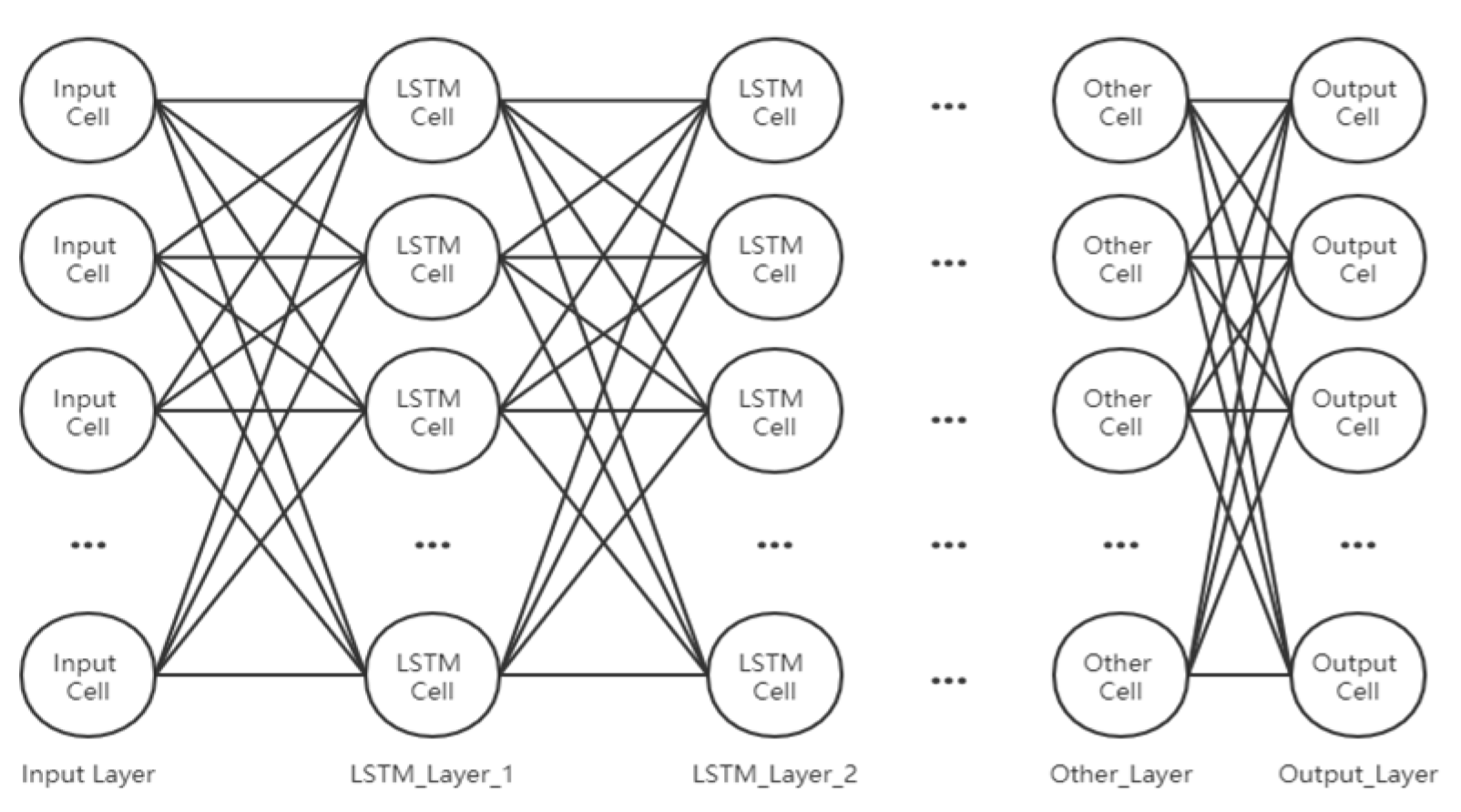
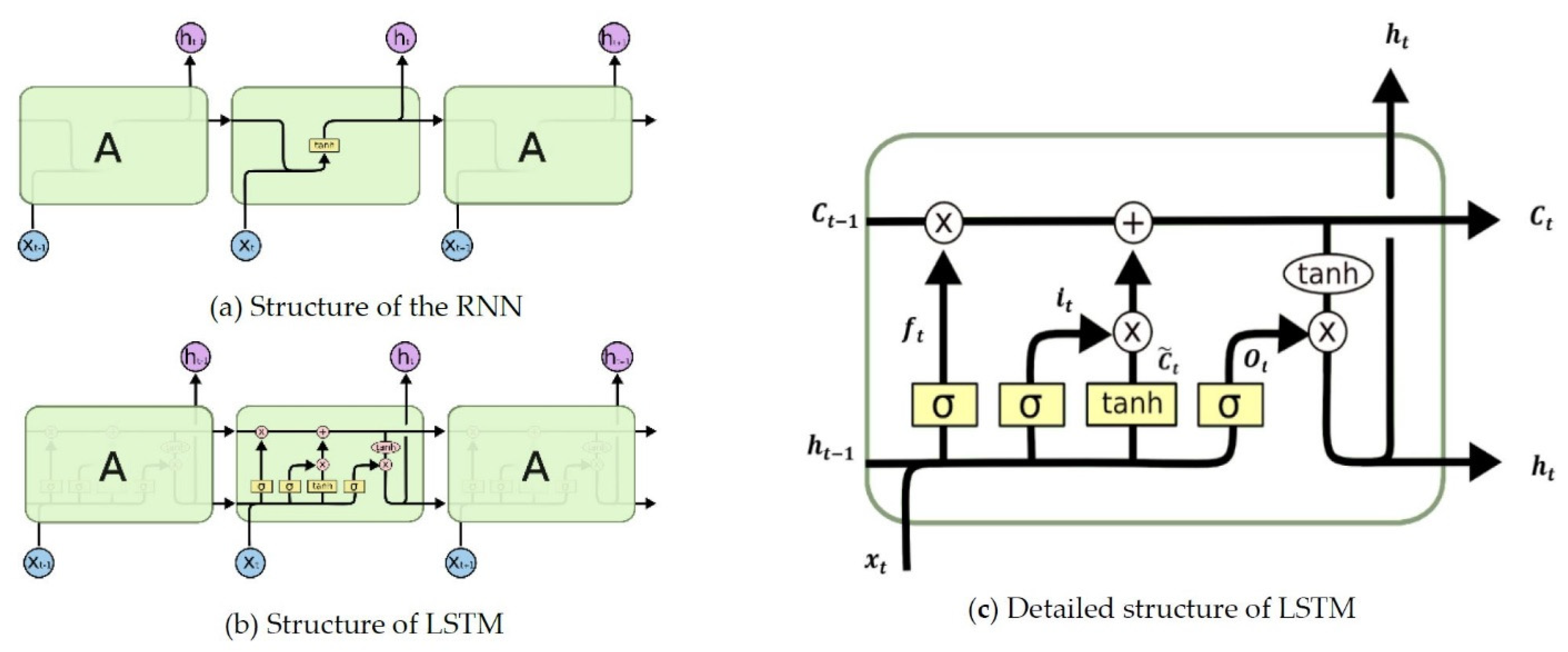
2.2. Long Short-Term Memory Model

The LSTM model (Hochreiter et al. [17]) is a variant of the recurrent neural network (RNN). The RNN cannot learn longer histories’ data, resulting in a gradient decline or even disappearance at further time steps. To solve this problem, the LSTM model introduces storage units and unit states to control information transfer based on the RNN.

There are four gates (forget gate, input gate, update gate and output gate) in the storage unit of the LSTM model. The input gate controls the addition of new information. The forget gate can forget information that needs to be discarded and retain the useful information of the past. The update gate can update data. The output gate causes the storage unit to output only information related to the current time step. These four gate structures perform matrix multiplication and non-linear summing in the memory cells so that the memory does not decay in constant iterations.

As shown in Figure 2, the structure of LSTM neural network consists of three layers: input layer, hidden layer (LSTM_Layer_1 and Other Layer) and output layer. Figure 3a shows the structure of the RNN. Its cell contains only one activation function, and the cells are only linked in order. Figure 3b is the structure of LSTM. Its cell is more complex than the RNN. It needs four gate calculations to output to the next cell. Figure 3c is an enlarged view of Figure 3b.

Forget Gate: For time t, the state $h_{t-1}$ at the previous time and the current training data $x_t$ can get $f_t$ through the forget gate; the formula is as follows:

$$f_t=\mathsf{\sigma }\left(W_f·\left[x_t,h_{t-1}\right]+b_f\right)$$

(15)

Input Gate: ${\tilde{C}}_t$ decides the amount that can be added to the cell state in the tanh network layer, and $i_t$ outputs a number between 0 and 1 through the Sigmoid network layer to decide which status values to update; the formula is as follows:

$$\widetilde{C_t}=tanh\left(W_c·\left[x_t,h_{t-1}\right]+b_c\right)$$

(16)

$$i_t=\mathsf{\sigma }\left(W_i·\left[x_t,h_{t-1}\right]+b_i\right)$$

(17)

Update Gate: Updates old state $C_{t-1}$ to new state $C_t$. This gate retains long-term and short-term memory in different proportions of the cell; the formula is as follows:

$$C_t=i_t\ast \widetilde{C_t}+f_t\ast C_{t-1}$$

(18)

Output Gate: The third sigmoid network layer determines parts of the output cell state, combined with Equation (20), to obtain the output value of the cell; the formula is as follows:

$$o_t=\mathsf{\sigma }\left(W_o·\left[x_t,h_{t-1}\right]+b_o\right)$$

(19)

$$h_t=o_t\ast {\theta }_h\left(C_t\right)$$

(20)

where $f_t$: forget gate, $\widetilde{C_t}$: input cell, $i_t$: input gate, $C_t$: update gate, $o_t$: output gate, σ: sigmoid activation function, W: weights for different gates, $x_t$: input value at time t, $h_{t-1}$: output value at the previous moment, and b: bias term for different gates.

2.3. $C{O}_2$ Emission Estimation Model

In this study, we adopted the ITTC recommended procedure [19,20] to estimate vessel resistance. It is necessary to derive the total resistance first. Total resistance can be denoted as:

$$R_T=\frac{1}{2}{C}_T\rho S{V}^2$$

(21)

where $R_T$: total resistance, $C_T$: total resistance coefficient, $\rho$: density of water, S: wetted surface of the hull, V: SOG.

$C_T$, the total resistance coefficient, can denoted as:

$$C_T=C_F+C_A+C_{AA}+C_R$$

(22)

where $C_F$: frictional resistance coefficient, $C_A$: incremental resistance coefficient, $C_{AA}$: air resistance coefficient, $C_R$: residual resistance coefficient.

Based on calculated total resistance of the vessel, an estimation of the required power for the vessel to sail at speed V in a calm sea condition can be calculated by considering the components of the propulsion efficiencies. Installed power is the power required to tow the vessel with speed V in a calm sea. Service power can be derived from:

$$P_I=\frac{R_{T}V}{\left({\eta }_T{\eta }_D\right)}+m$$

(23)

where $P_I$: installed power, ${\eta }_T$: transmission efficiency,${\eta }_D$: quasi-propulsive coefficient, m: sea margin.

Fuel oil consumption is calculated by using the specific fuel oil consumption (SFOC) as shown in

Table 1. Specific fuel oil consumption (SFOC) and distribution of engine age of vessels included in automatic identification system (AIS) data.

Engine Age	Slow-Speed Diesel (SSD) Engine	Medium-Speed Diesel (MSD) Engine	High-Speed Diesel (HSD) Engine
Before 1983	205	215	225
1984–2000	185	195	205
Post–2001	175	185	195

from Smith et al. [21]. Table 1 shows the value of the SFOC for each diesel engine type with engine age. As the vessel engine becomes older, the efficiency of the engine decreases and the advent of technology makes a newer engine more efficient.

The marine liquefied natural gas (LNG) ${\mathrm{CO}}_2$ emissions factor is 2.75. So, the ${\mathrm{CO}}_2$ emission estimation model can be denoted as:

$$E_i={{\displaystyle \sum }}^{}{P}_I\times SFOC\times 2.75\times T$$

(24)

where $E_i$, the total ${\mathrm{CO}}_2$ emissions, is calculated by summing the carbon dioxide emissions at each trajectory point; T is the time interval of each track point.

3. Experiments and Results

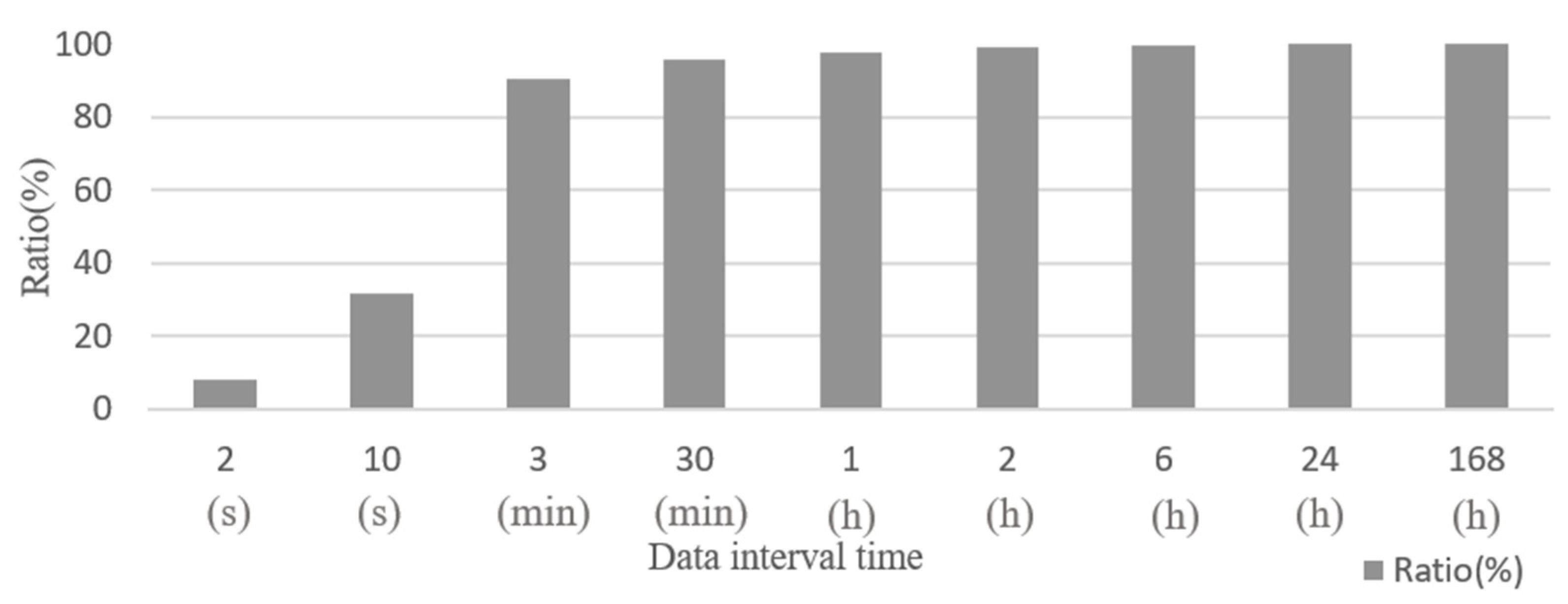
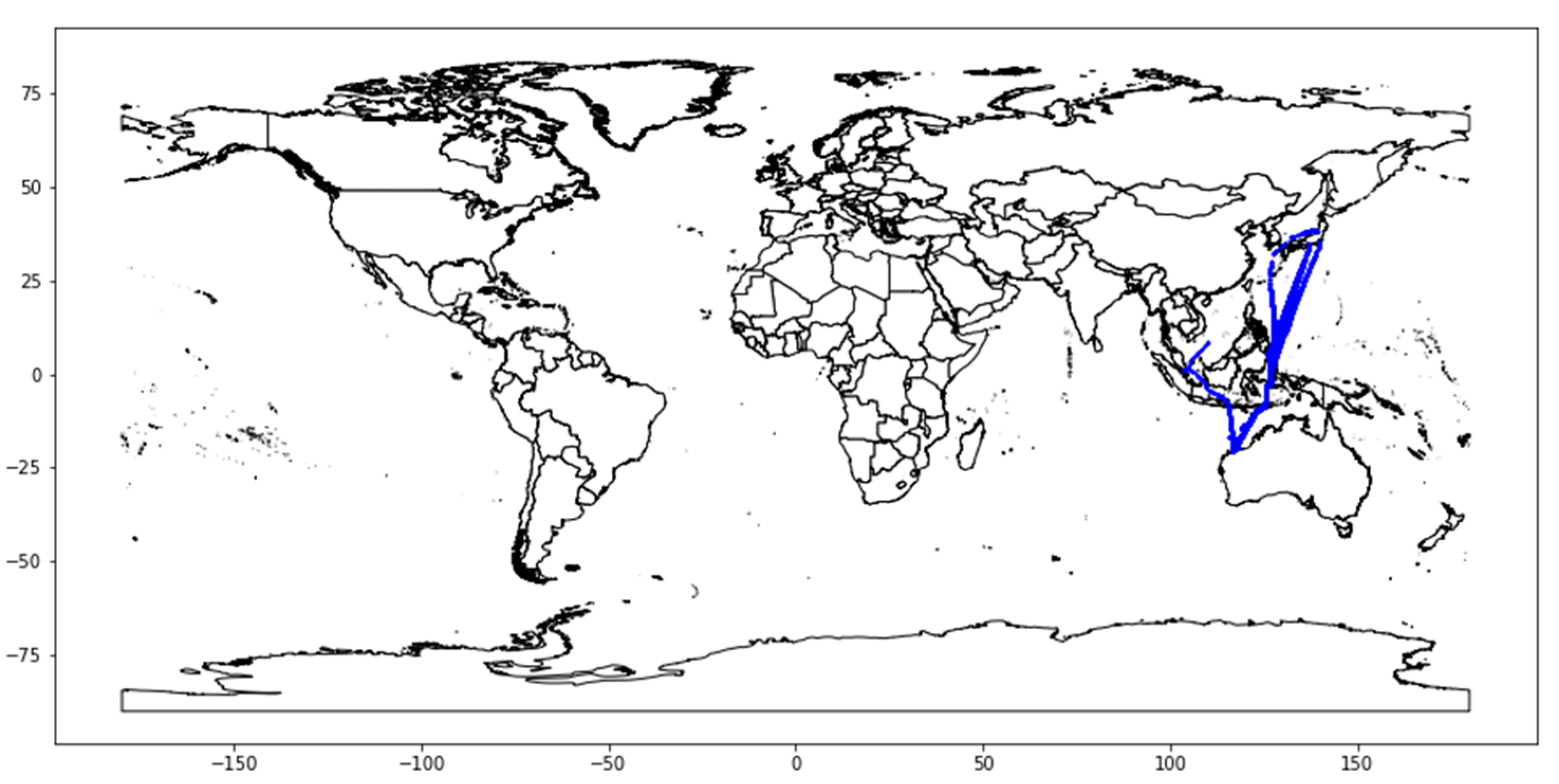
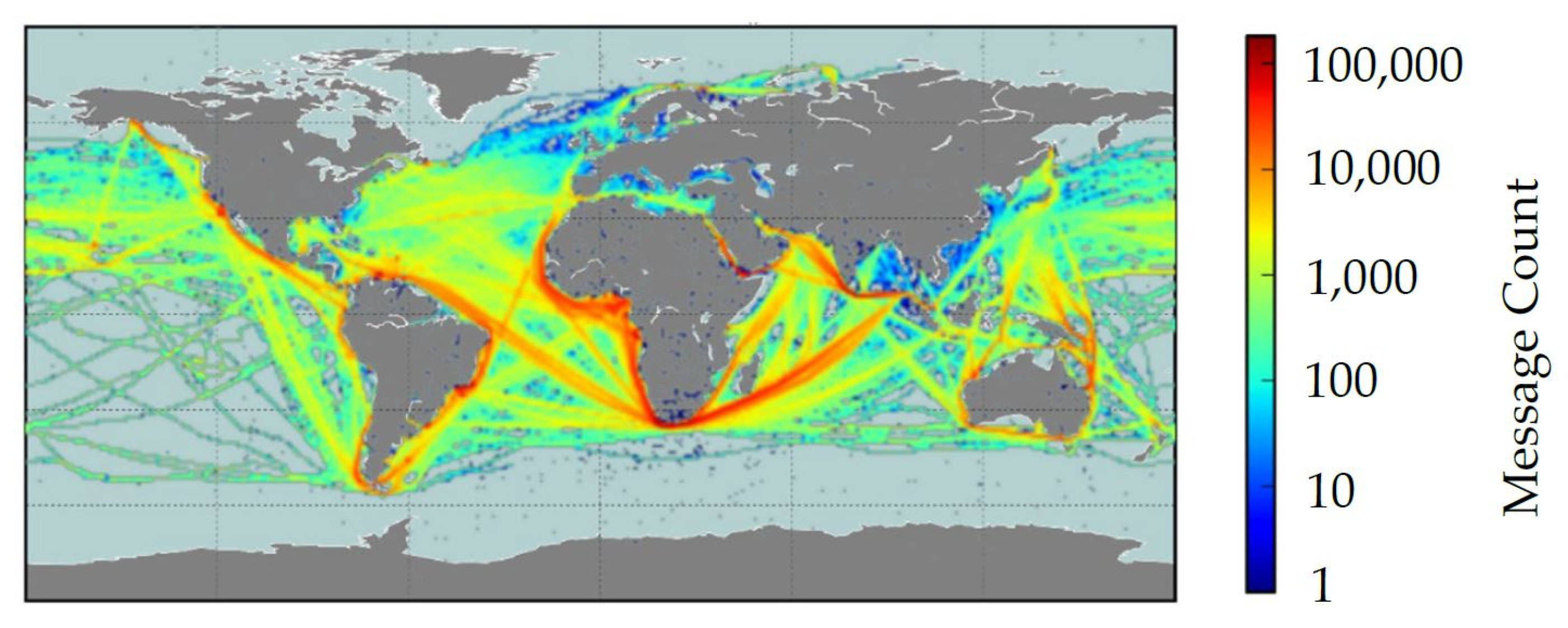
3.1. Automatic Identification System (AIS) Dataset Analysis

This study used AIS data of an LNG vessel provided by exactEarth, as shown in Figure 4. The time period was from 1 January 2016 to 30 June 2016, and number of messages was about 50 million. It included vessel names, callsigns, maritime mobile service identities (MMSIs), vessel types, vessel cargos, vessel classes, lengths, widths, flag countries, destinations, estimated times of arrival (ETAs), draughts, longitudes, latitudes, SOGs, COGs, rates of turn (ROTs), headings, navigation (nav) statuses, source, times, main vessel types and sub vessel types.

The AIS data used this research took a comma-separated values (CSV) form. Every datum was divided by day based on Greenwich Mean Time (GMT). A total of 182 days were included, so the complete data of the vessel were divided into 182 small datasets. This was inconvenient, so we used MySQL to build a trajectory database combining the 182 small datasets into a large dataset.

This trajectory dataset mainly included: MMSI, longitude, latitude, SOG, COG and time.

In the original dataset, we found that the average time interval of each piece of AIS data in

Table 2. Summary statistics of data interval.

Items	Hour	Minutes	Seconds
Count (number)	9,072,291	9,072,291	9,072,291
Mean	0.14	8.68	520.52
25%	0.00	0.10	6.00
50%	0.00	0.28	17.00
75%	0.01	0.70	42.00

was 520.52 s. Furthermore, 25% of the data had an interval time within 6 s, 50% were within 17 s, and 75% were within 42 s. According to Figure 5, we also found that more than 90% of the data had a time interval of more than 30 min. Only about 8% of the data had a time interval of 2 s. This may be because AIS data collected through satellites show longer data collecting intervals when the vessel was sailing in areas with high traffic compared to areas with less traffic.

3.2. Interpolation Calculation

After database analysis, taking the data integrity and continuity as the principle, we extracted the LNG vessel trajectory data of MMSI 310028000 from the trajectory database as a sample to illustrate the feasibility of the model. The vessel trajectory over six months is shown in Figure 6. The vessel travels mainly between Japan and Australia; the IMO number is “8913174”, built in 1992.

The focus of this research was to grasp the carbon dioxide emissions of vessels in real-time. We chose to use vessel data from 5 January 2016 over 00:35:10–00:59:40 for analysis. The reason for the selection was that the AIS data has relatively larger data points during the period, which could minimize the workload of trajectory data reconstruction. In addition, the trajectory trend is a straight line instead of a curve, which is more appropriate for simplicity. The total time interval was 26 min, and there were 23 trajectory data points, as shown in

Table 3. Partial sample data.

MMSI	Time	Longitude	Latitude	SOG	COG
310028000	00:35:10	118.6957	−17.0403	15.9	24.7
310028000	00:35:11	118.6961	−17.0395	15.8	25.1
310028000	00:35:18	118.6963	−17.0391	15.9	25.1
310028000	00:35:29	118.6966	−17.0383	15.8	25
310028000	00:35:41	118.697	−17.0375	15.8	24.8
310028000	00:35:48	118.6972	−17.0371	15.8	25.2

. For example, we found that the data intervals were different: 1 s, 7 s, 11 s, 12 s, 7 s from 00:35:10 to 00:35:48. Therefore, this study proposes using the cubic spline interpolation method to resample the data at one second intervals.

We used Equations (1)–(14) to calculate the trajectory interpolation. Taking longitude as an example,$x_i=longitud{e}_i$. The partial calculation results are shown in Figure 7. We found that the line connecting the original data points was no longer a simple straight line (orange color), but had become a curve (blue color), which was more in line with the actual situation. In terms of the actual geographic location, we could see the restored trajectory after interpolation calculation from Figure 8, where the yellow point is the trajectory point of the vessel at 00:59:40, the red point is the trajectory point on 5 January, the orange point is on other days in January and the green points are interpolation points.

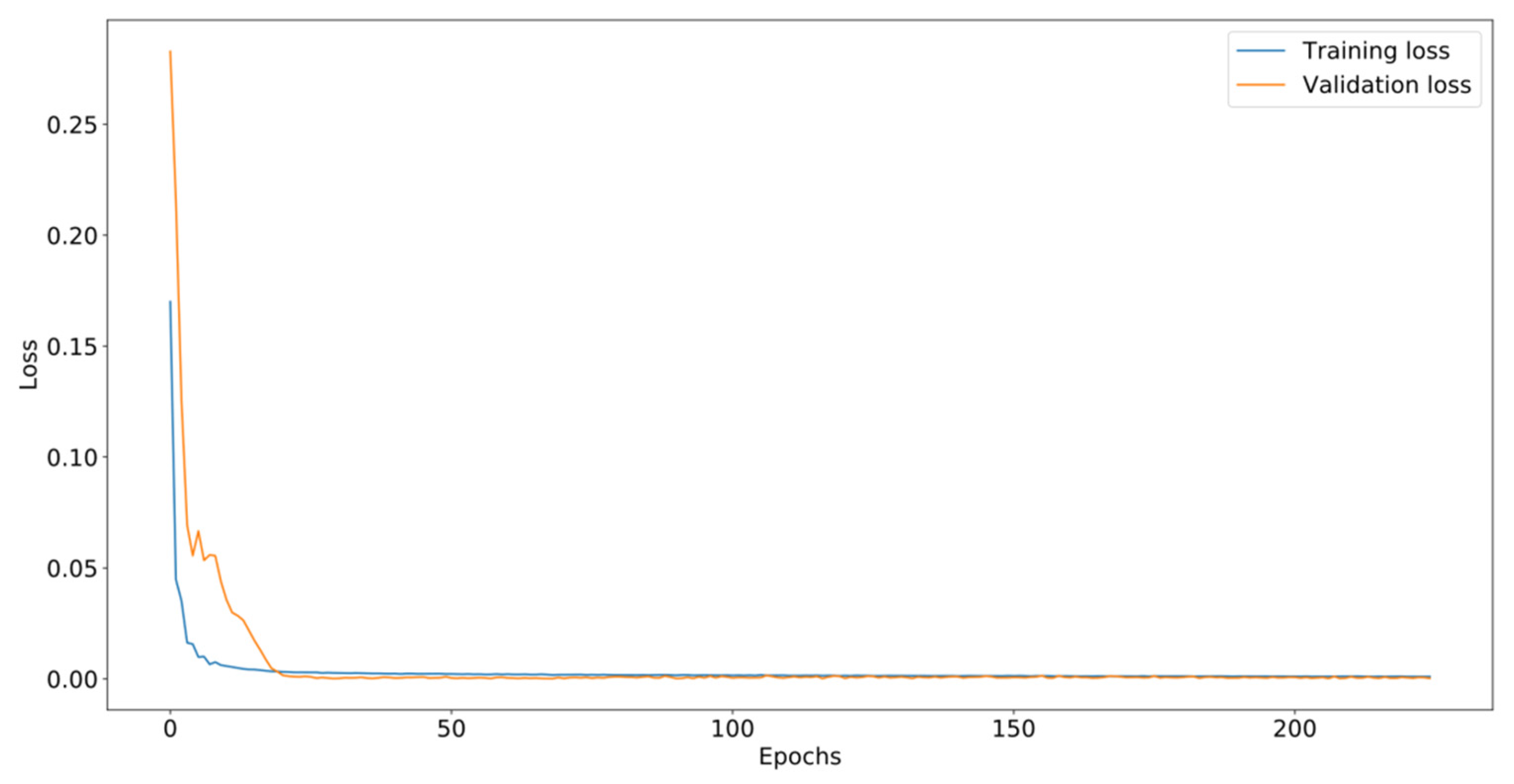
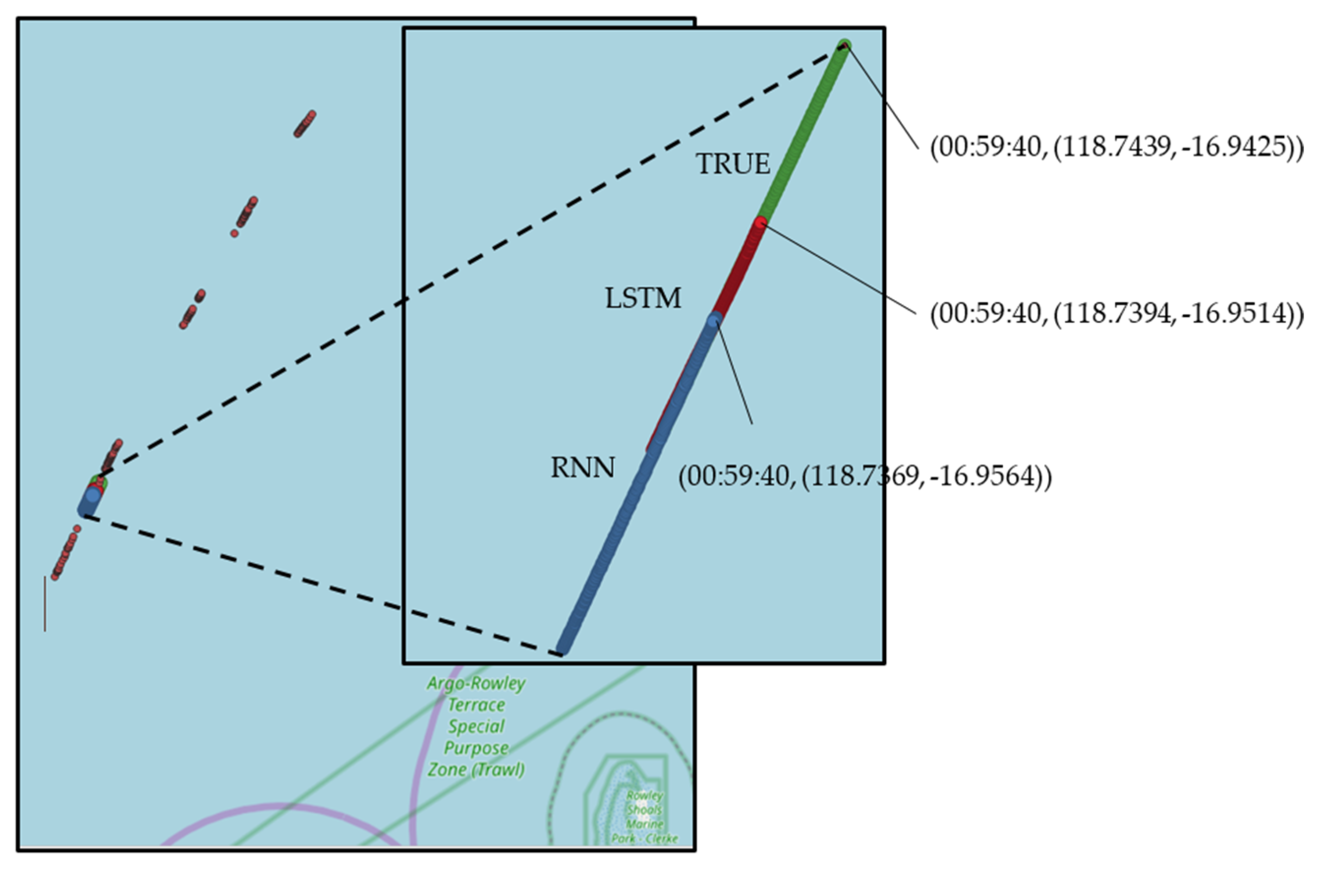
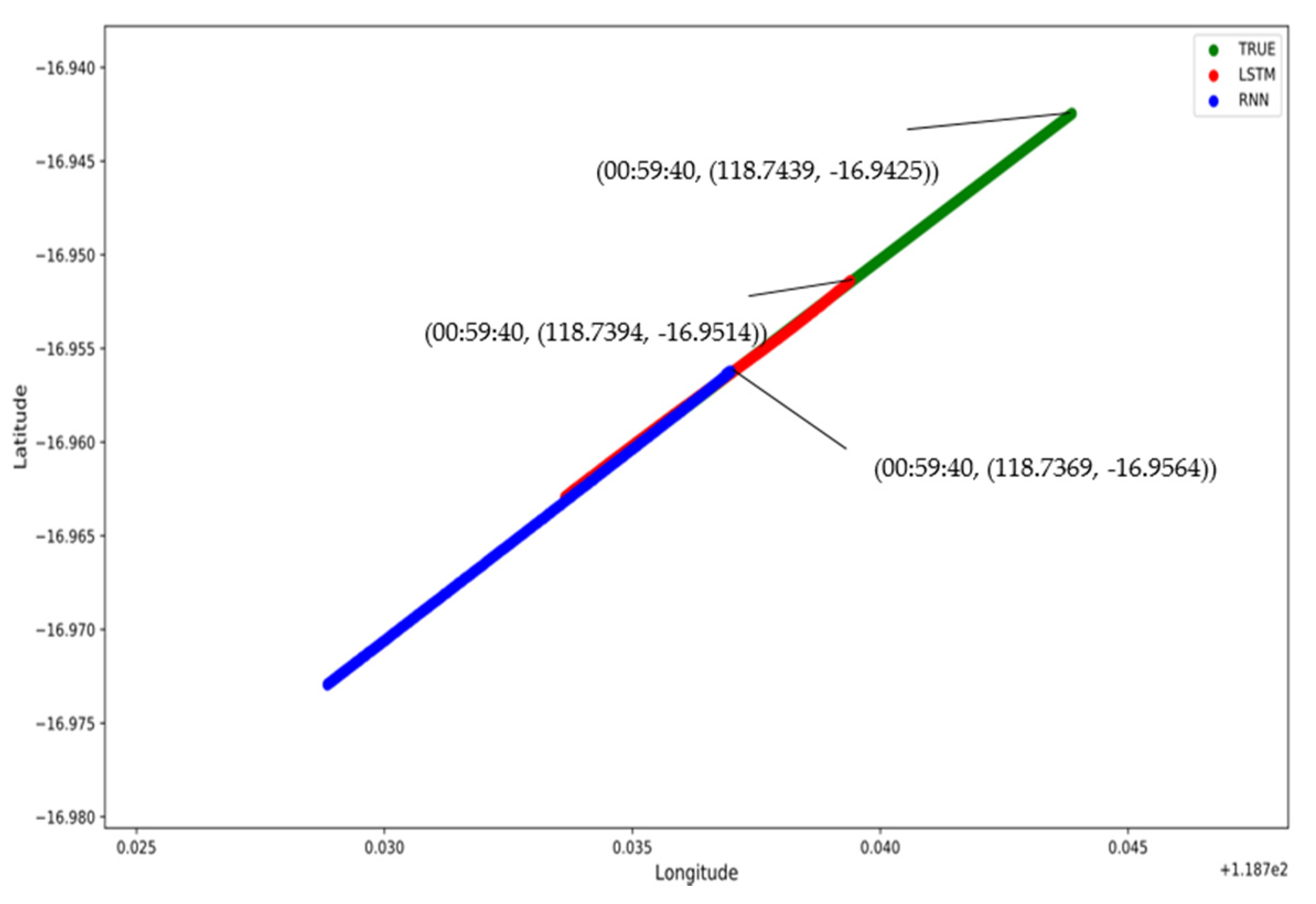
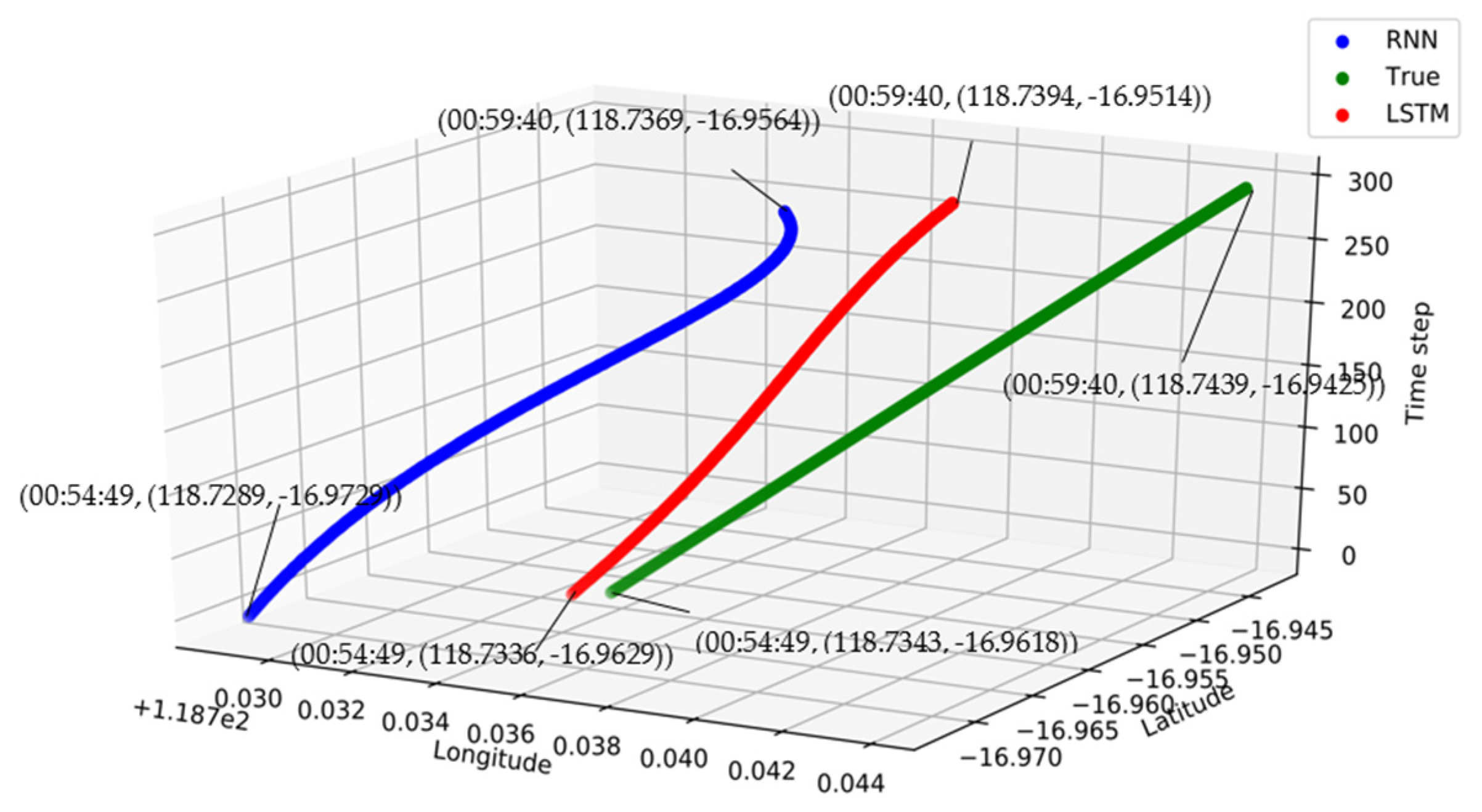
3.3. Vessel Trajectory Prediction

The recurrent neural network is a typical framework for deep learning; it can be used to deal with spatial–temporal sequence problems. The characteristics are that the output of the current moment depends on the calculation result of the previous moment and that the timing is strong. The LSTM model is an improvement on the recurrent neural network as it also analyzes historical calculation results that are much older, automatically removes invalid historical calculation results, and remembers useful historical calculation results by introducing gating functions. The timeliness is stronger than the recurrent neural network.

As described in Section 1.2, for a vessel, its trajectory characteristics at time t could be expressed as $Y_{\left(t\right)}=$ {($p_1,a_1,t_1$),($p_2,a_2,t_2$),($p_3, a_3,t_3$),…,($p_n,a_n,t_n$)}; we could use this as an input value of the LSTM model. The number of data after the interpolation calculation changed from 23 to 1472. The experimental environment for this study was the DELL OptiPlex 7050 desktop computer, the CPU was Intel(R) Core (TM) i7-7700 CPU @3.60GHz, the memory was 16.0 GB, the operating system was Windows10 Pro, the program development environment was PyCharm (JetBrains, s.r.o., Prague, Czech Republic) in python 3.7 and we used an LSTM model provided by Keras (Chollet, F., & others, Retrieved from https://github.com/fchollet/keras (accessed on 20 July 2021)). After experiments and manual adjustment of parameters, the optimal parameters of the LSTM model in this study were finally determined. As shown in

Table 4. LSTM model parameters.

Items	Parameters	Items	Parameters
Base Learning Rate	0.001	LSTM_layer_1	256
Optimizer	Adaptive moment estimation	LSTM_layer_2	128
Epoch	125	Dropout_layer _1	128
Batch size	138	Dense_layer _1	128
Loss function	Mean square error	Dropout_layer _2	128
Activation_1	Tanh	Dense_layer _2	4
Activation_2	Linear	Kernel_initializer	Orthogonal
Train set	938	Validation set	235
Test set	293	-	-

, the time required to run the model once was 195 s.

The loss function is shown in Figure 9. We used 938 pieces of data to train the LSTM model, and finally, 235 pieces of data were used to verify the prediction effect. At an equal time (00:59:40), the predicted trajectory point of the LSTM model differed from the actual trajectory point by 0.593 nm, which was in line with expectations.

The prediction results are shown in Figure 10, and we further plot these in 2D (Figure 11) and 3D (Figure 12) graphs for visualization.

As Figure 10 shows, the trajectories predicted by the two models roughly coincided with the actual trajectories. In Figure 11 and Figure 12, the green, red and blue lines indicate the trajectory points of the vessel during the period of study, where the green line indicates the true trajectory point, the red point indicates the trajectory point predicted by the LSTM model and the blue point represents trajectory point predicted by the RNN model. The trajectory point predicted by the LSTM (118.7394, −16.9514) is closer to the true value (118.7439, −16.9425) than the trajectory point predicted by the RNN model (118.7369, −16.9564).

In Figure 11, we intercepted the prediction result from original trajectory to visualize the differences. Three trajectories had the same start point (the first orange point at the lower left in Figure 10) but the predicted endpoints were different. The LSTM model has a smaller error (0.593 nautical miles or 1.097 km) than that of the RNN model (0.928 nautical miles or 1.718 km). This can be observed in Figure 12 where the trajectory predicted by the RNN was more concentrated at the end point, causing the trajectories to overlap, while the LSTM model did not have this defect. The time step was the time difference from 00:54:49 (in seconds).

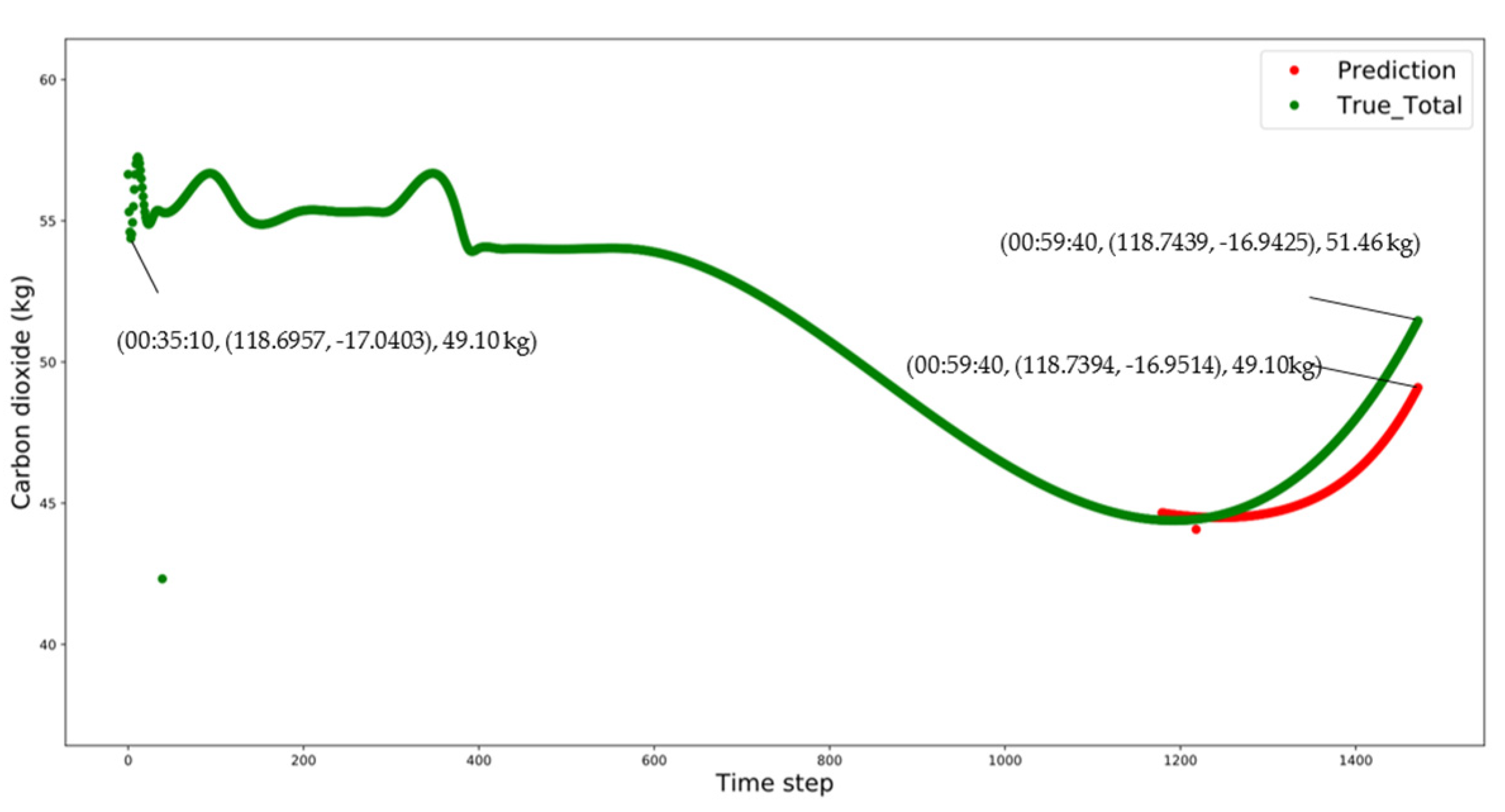
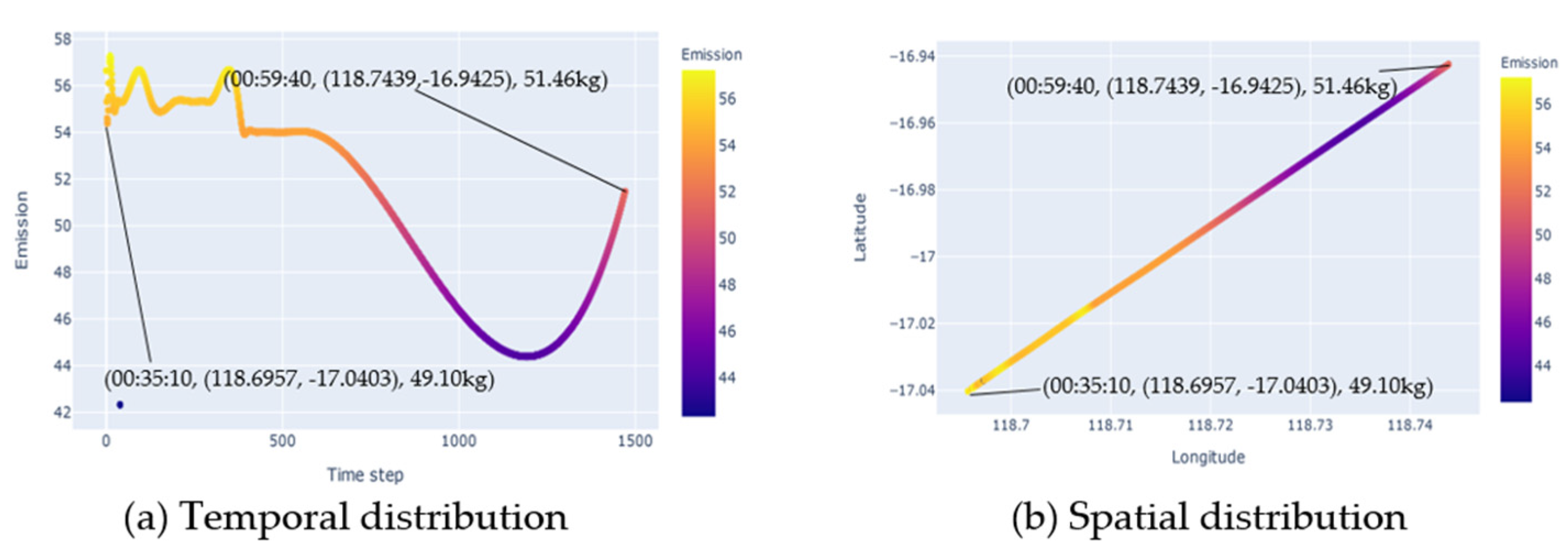
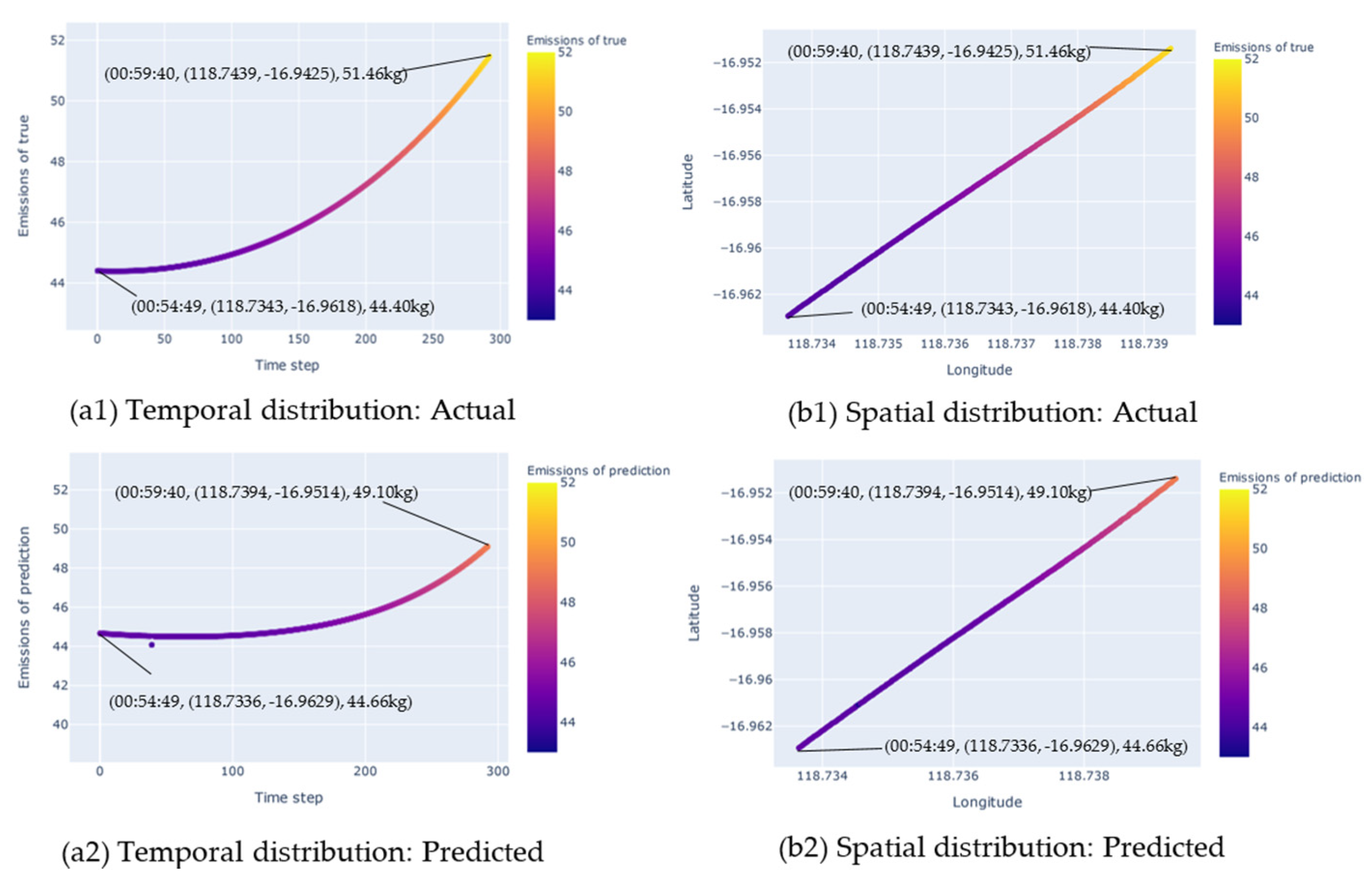
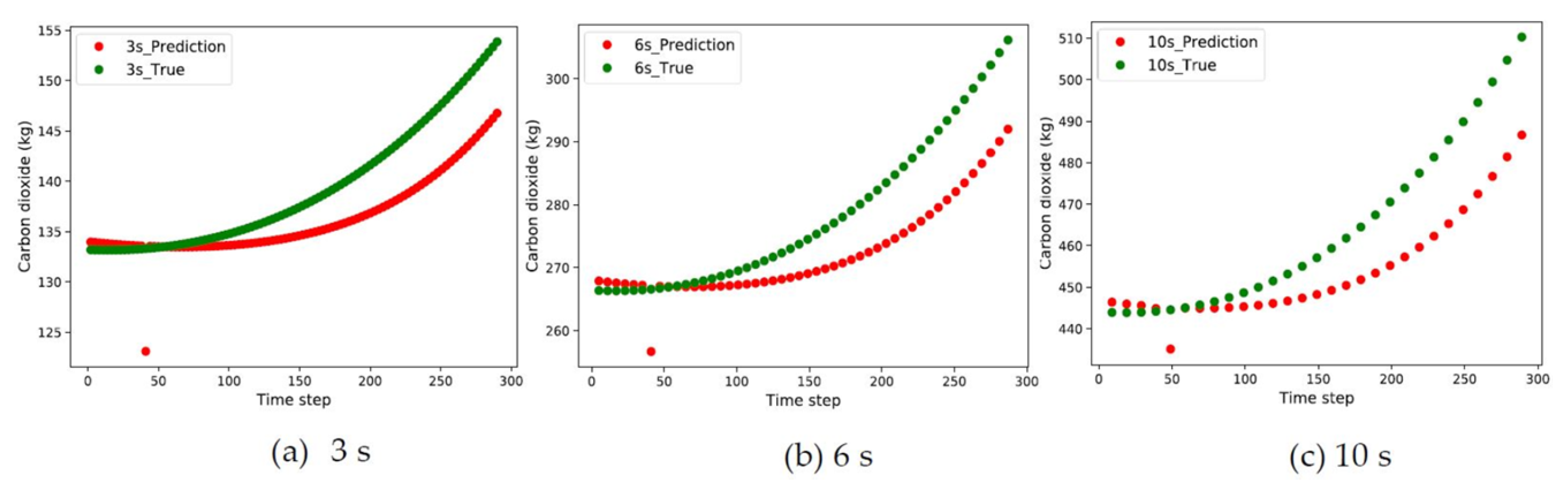
3.4. Carbon Dioxide Estimation

We first calculated the carbon dioxide emissions of the vessel without interpolation by the ITTC; using Equation (24), we could determine the emissions of the vessel at 00:35:10–00:59:40 to be 47,169 kg for the period of study. The carbon dioxide emissions after interpolation totaled 74,926 kg for the same period. This was 27,757 kg more carbon dioxide emissions than determined by traditional estimation methods. Our proposed model was able to interpolate more time intervals, and hence, improve the accuracy of the vessel carbon dioxide emissions. Observing the vessel carbon dioxide emissions from a spatial–temporal perspective, they go down first and then up (Figure 13 and Figure 14).

Next, we used the trajectories predicted by the LSTM model to estimate the carbon dioxide emissions, to obtain the spatial–temporal distribution of future carbon dioxide emissions from vessels. With the vessel emissions per second obtained, we calculated that the cumulative carbon dioxide emissions from vessels during 00:54:49–00:59:41 were 13,315 kg. We predicted that the highest value would be reached in this area (118.7439, −16.9425).

The predicted carbon dioxide emissions (13,315 kg) and the true emissions (13,616 kg) gave an error of 301 kg. A heat map is shown of the spatial–temporal distribution of carbon dioxide emissions from vessels every second in specific section from 00:54:49 to 00:59:40 in Figure 15. Observing the vessel carbon dioxide emissions from a time perspective, the actual and predicted values increased during this period. We found that the growth rate of the predicted value was slower than the growth rate of the true value. At 00:59:41, the error was 2.36 kg (51.46–49.10 kg).

Moreover, it was found that the vessel emissions in the future would continue to increase. The deceleration trend indicated that the vessel would accelerate to the northeast in the future. On the other hand, because we had the data of the carbon dioxide emissions of the vessel in seconds, we could re-establish any time interval to reduce the number of vessel trajectory points if needed. That practice is useful for calculating a larger number of vessel carbon emission trajectories, for example, to calculate the carbon dioxide emissions of the vessel in 3 s, 6 s or 10 s intervals (Figure 16). We can see from Figure 16 that the larger the number of time steps, the faster increase of carbon dioxide emissions, which also indicates that the SOG of the vessel was accelerating. At the same time, the number of trajectory points decreased as the time interval decreased, and the vessel carbon dioxide emissions represented by each track point gradually increased, but the overall trajectory trend remained the same.

4. Conclusions

In this study, we proposed a method to interpolate AIS data and estimate vessel emissions based on predicted vessel trajectories using deep learning models. The results suggest that the carbon dioxide emissions are underestimated. The method can be applied to monitor a vessel’s carbon dioxide emissions and trajectory in real time, and to provide vessels with early warning services relating to carbon dioxide emissions monitoring.

The contributions of the study are fourfold. Firstly, it has novelty in interpolating AIS data points with a non-linear model. AIS data sometimes have time intervals that are too long due to equipment issues and/or human reasons, which limits the accuracy of the vessels’ carbon dioxide emissions estimation based on AIS data. To overcome the problem, this study proposes a cubic spline interpolation model to resample missing AIS data points. The repaired trajectories of the vessel (Figure 8) maintain the same trend as the original trajectory in smooth curves, which represent the actual situation well when compared to the traditional linear models in previous studies. Through the interpolation, we could successfully obtain AIS data with a time interval of one second.

Secondly, it reveals that vessel emissions are currently underestimated. In the study, by applying the repaired trajectory data of the vessel (1472 pieces of data), we estimated the carbon dioxide emissions of the vessel to be 74,926 kg. Compared to the emissions calculated from the original trajectory data (23 pieces of data), a 27,757 kg increase of carbon dioxide emissions was identified. This clearly indicates that the actual carbon dioxide emissions are higher than those reported. The finding offers insight into how to accurately measure the emissions of vessels, and hence, better execute a GHG reduction strategy.

Thirdly, it validated the performance of two deep-learning algorithms in predicting vessel trajectories. We conducted prediction with two deep-learning algorithms, LSTM and RNN. The results confirm that the LSTM model performs better. We used the predicted SOG to predict the future carbon dioxide emissions of the vessel. The error was as small as 301 kg, which shows that the LSTM model was suitable for spatial–temporal data prediction with excellent performance.

Fourthly, it offers an alternative solution to predict vessel trajectories when AIS data is not retrievable. The model can also be used to estimate vessel emissions when AIS data are not available on occasions such as the shutdown of AIS for artificial reasons (including active or passive) or when the collection of AIS data fails in certain time periods.

At present, the method has limitations since it has only been tested in cases where the vessel trajectory is not comprehensive. It is unclear about the interpolation effect and trajectory prediction effect on curved trajectories, which need further research with several cases considering the computational time in the future. Future studies may also verify different artificial neural network (ANN) models such as the feedforward neural network (FFNN) or 1D convolutional neural networks (1D-CNN), which may work well on time-series data [14].

References

1. Mabunda, A.; Astito, A.; Hamdoune, S. Estimating Carbon Dioxide and Particulate Matter Emissions from Ships using Automatic Identification System Data. Int. J. Comput. Appl. 2014, 88, 27–31. [Google Scholar]
2. Winther, M.; Christensen, J.H.; Plejdrup, M.S.; Ravn, E.S.; Eriksson, O.F.; Kristensen, H.O. Emission inventories for ships in the arctic based on satellite sampled AIS data. Atmos. Environ. 2014, 91, 1–14. [Google Scholar] [CrossRef]
3. International Maritime Organization (IMO). MEPC 75/7/15: Reduction of GHG Emissions from Ships: Fourth IMO GHG Study 2020—Final Report; International Maritime Organization (IMO): London, UK, 2020. [Google Scholar]
4. Coello, J.; Williams, I.; Hudson, D.A.; Kemp, S. An AIS-based approach to calculate atmospheric emissions from the UK fishing fleet. Atmos. Environ. 2015, 114, 1–7. [Google Scholar] [CrossRef]
5. Yao, X.; Mou, J.; Chen, P.; Zhang, X. Ship emission inventories in estuary of the Yangtze River using terrestrial AIS data. TransNav 2016, 10, 633–640. [Google Scholar] [CrossRef] [Green Version]
6. Wang, Z.H.; Wang, W.X.; Shi, X. AIS data-based ship emission estimation model and real ship verification. J. Shanghai Marit. Univ. 2019, 40, 12–16. [Google Scholar]
7. Kim, H.; Watanabe, D.; Toriumi, S.; Hirata, E. Spatial Analysis of an Emission Inventory from Liquefied Natural Gas Fleet Based on Automatic Identification System Database. Sustainability 2021, 13, 1250. [Google Scholar] [CrossRef]
8. Laxhammar, R.; Falkman, G.; Sviestins, E. Anomaly detection in sea traffic—A comparison of the Gaussian Mixture Model and the Kernel Density Estimator. In Proceedings of the 12th International Conference on Information Fusion, Seattle, WA, USA, 6–9 July 2009; pp. 756–763. [Google Scholar]
9. Zhao, S.B.; Tang, C.; Liang, S.; Wang, D. Track prediction of vessel in controlled waterway based on improved Kalman filter. J. Comput. Appl. 2012, 32, 3247–3250. [Google Scholar] [CrossRef]
10. Quan, B.; Yang, B.; Guo, C.; Li, Q. Prediction Model of Ship Trajectory Based on LSTM. Comput. Sci. 2018, 45, 126–131. [Google Scholar]
11. Nguyen, D.D.; Le Van, C.; Ali, M.I. Vessel trajectory prediction using sequence-to-sequence models over spatial grid. In Proceedings of the 12th ACM International Conference on Distributed and Event-based Systems, Hamilton, New Zealand, 25–29 June 2018; pp. 258–261. [Google Scholar]
12. Ljunggren, H. Using Deep Learning for Classifying Ship Trajectories. In Proceedings of the 21st International Conference on Information Fusion (FUSION), Cambridge, UK, 10–13 July 2018; pp. 2158–2164. [Google Scholar]
13. Wang, L.L.; Liu, J. Ship behavior recognition method based on multi-scale convolution. J. Comput. Appl. 2019, 39, 3691–3696. [Google Scholar]
14. Theodoropoulos, P.; Spandonidis, C.C.; Themelis, N.; Giordamlis, C.; Fassois, S. Evaluation of Different Deep-Learning Models for the Prediction of a Ship’s Propulsion Power. J. Mar. Sci. Eng. 2021, 9, 116. [Google Scholar] [CrossRef]
15. Theodoropoulos, P.; Spandonidis, C.C.; Giordamlis, C.; Fassois, S. Stability and Safety of Ships and Ocean Vehicles Enhancing vessel ’s operational safety using Convolutional Neural Networks and Big Data techniques. In Proceedings of the 1st International Conference on the Stability and Safety of Ships and Ocean Vehicles (STAB&S), Online, Glasgow, UK, 6–11 June 2021. [Google Scholar]
16. Bartels, R.; Beatty, J.; Barsky, B. Hermite and Cubic Spline Interpolation: Chapter 3. In An Introduction to Splines for Use in Computer Graphics and Geometric Modelling; Morgan Kaufmann: Burlington, MA, USA, 1995; pp. 9–17. [Google Scholar]
17. Hochreiter, S.; Schmidhuber, J. Long Short-Term Memory. Neural Comput. 1997, 9, 1735–1780. [Google Scholar] [CrossRef] [PubMed]
18. Olah, C. Understanding LSTM Networks. 2015. Available online: https://colah.github.io/posts/2015-08-Understanding-LSTMs/ (accessed on 7 August 2021).
19. International Towing Tank Conference. ITTC—Recommended Procedures and Guidelines; Procedure 7.5-02-02-01, Revision 04; ITTC Association: Zürich, Switzerland, 2017. [Google Scholar]
20. Molland, A.F.; Turnock, S.R.; Hudson, D.A. Ship Resistance and Propulsion: Practical Estimation of Ship Propulsive Power, 2nd ed.; Cambridge University Press: Cambridge, UK, 2017. [Google Scholar]
21. Smith, T.W.P.; Jalkanen, J.P.; Anderson, B.A.; Corbett, J.J.; Faber, J.; Hanayama, S.; O’Keeffe, E.; Parker, S.; Johansson, L.; Aldous, L.; et al. Third IMO GHG Study 2014; International Maritime Organization: London, UK, 2015. [Google Scholar]
Figure 1. Flow chat of this study.
Jmse 09 00871 g001
Figure 2. Structure of long short-term memory (LSTM) neural network.
Jmse 09 00871 g002
Figure 3. Structure of recurrent neural network (RNN) and LSTM cells. Source: adapted from Olah [18] with permission from Olah, C., 2021.
Jmse 09 00871 g003
Figure 4. Heat map of data.
Jmse 09 00871 g004
Figure 5. Distribution of data interval time.
Jmse 09 00871 g005
Figure 6. Distribution of sample vessel trajectory.
Jmse 09 00871 g006
Figure 7. Distribution of longitude interpolation.
Jmse 09 00871 g007
Figure 8. Geographical distribution of trajectory interpolation.
Jmse 09 00871 g008
Figure 9. Training and validation loss of LSTM model.
Jmse 09 00871 g009
Figure 10. Geographical distribution of predicted results.
Jmse 09 00871 g010
Figure 11. Coordinate distribution of true trajectory and predicted trajectory results (2D).
Jmse 09 00871 g011
Figure 12. Spatial–temporal distribution of true trajectory and predicted trajectory results (3D).
Jmse 09 00871 g012
Figure 13. Temporal distribution of total true and predicted results in comparison.
Jmse 09 00871 g013
Figure 14. Spatial–temporal distribution of total true results.
Jmse 09 00871 g014
Figure 15. Spatial-temporal distribution of true and predicted results for specific section.
Jmse 09 00871 g015
Figure 16. Spatial distribution of true and predicted carbon dioxide emissions with time intervals.
Jmse 09 00871 g016