
Numerical Study of the Dynamic Stall Effect on a Pair of Cross-Flow Hydrokinetic Turbines and Associated Torque Enhancement Due to Flow Blockage


Abstract
:1. Introduction
2. Blockage Effect on a Single Turbine
2.1. Materials and Methodology
2.1.1. Turbine Geometry
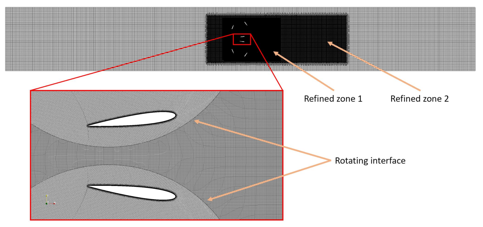
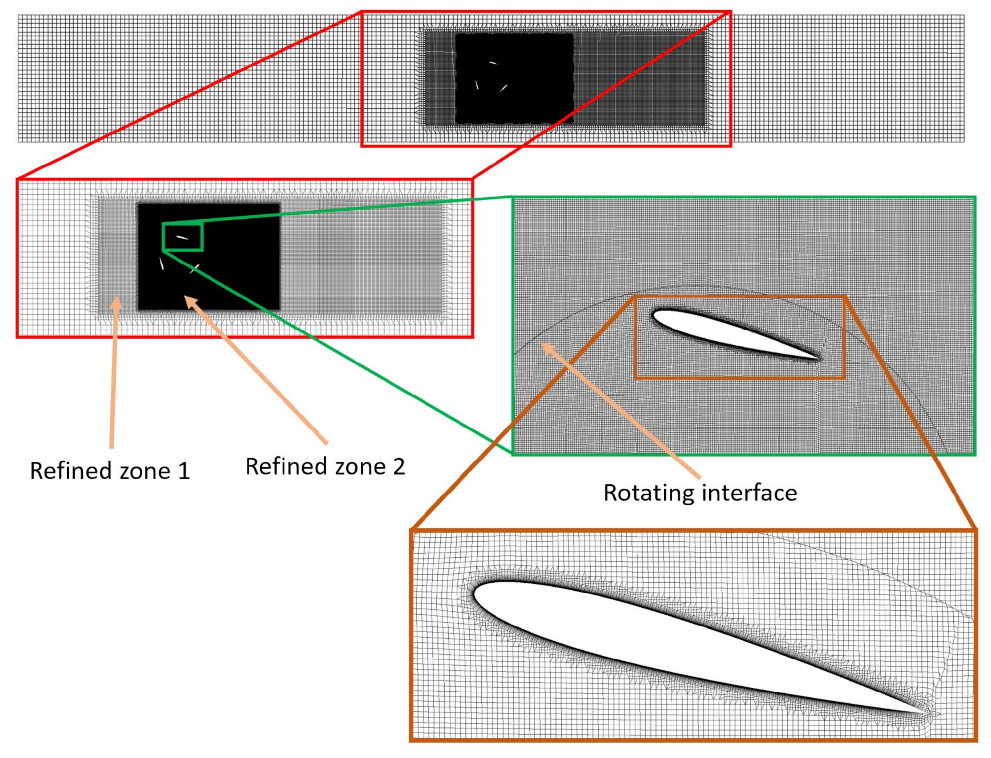
2.1.2. Pre-Processing
2.1.3. Turbulence Model, Boundary Conditions, and Numerical Schemes
2.2. Sensitivity Analysis
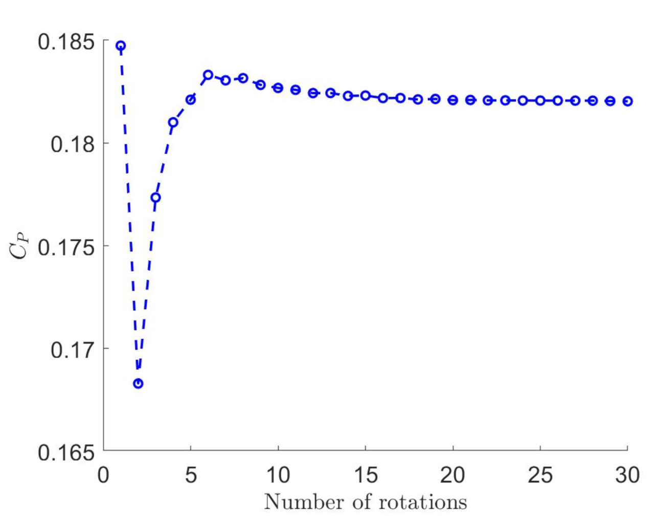
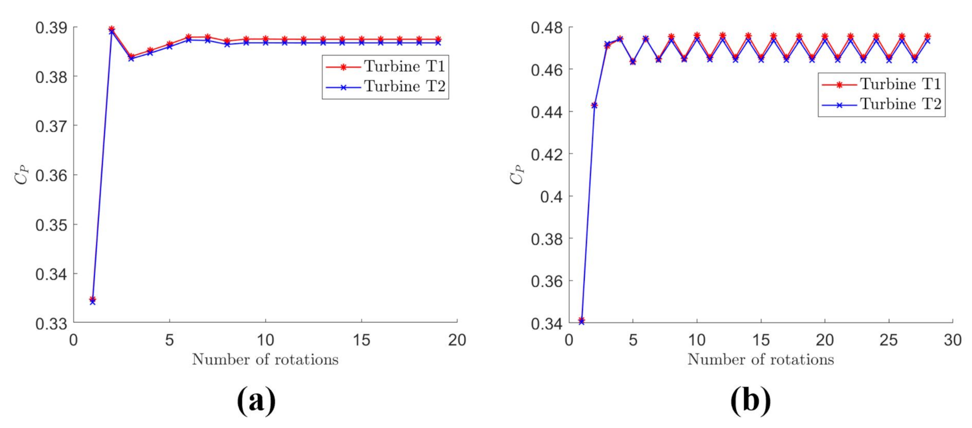
2.2.1. Convergence Criterion
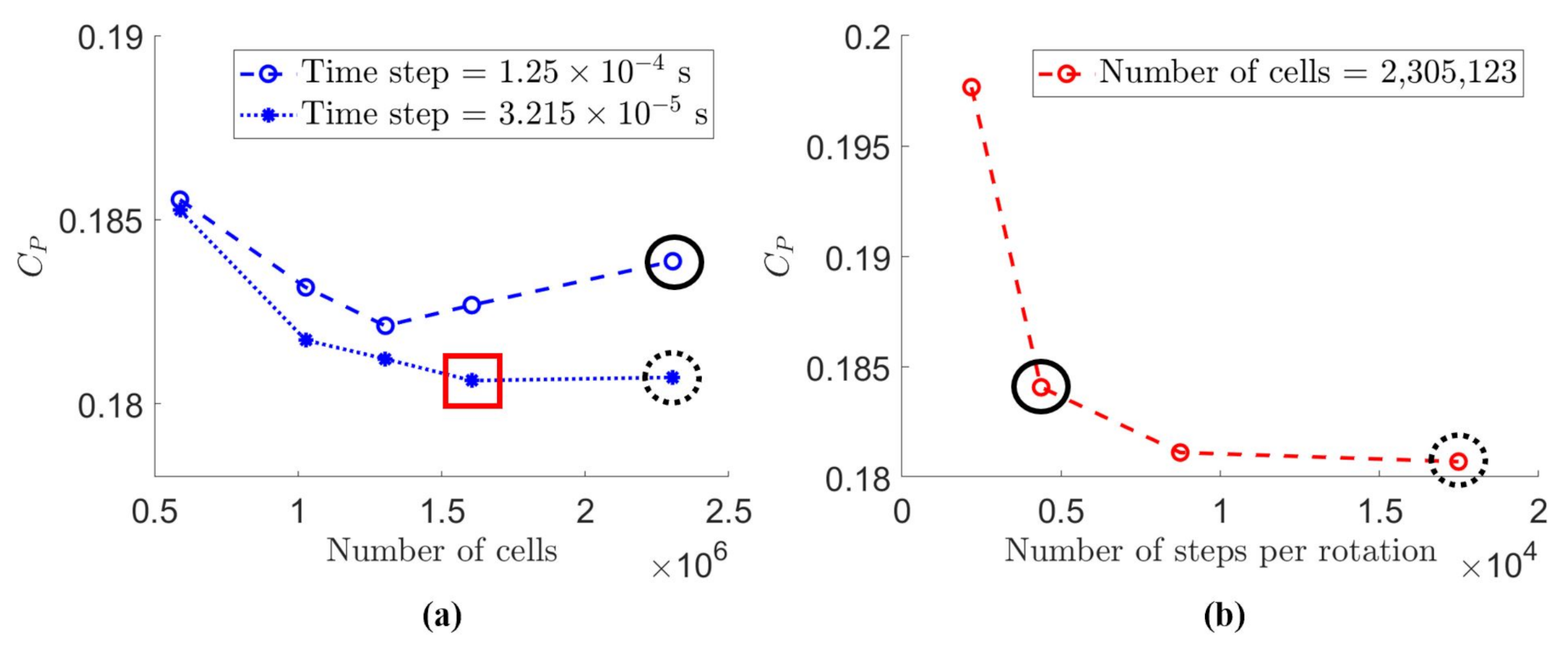
2.2.2. Iterative Spatial and Temporal Sensitivity Analysis
2.3. Results and Discussion
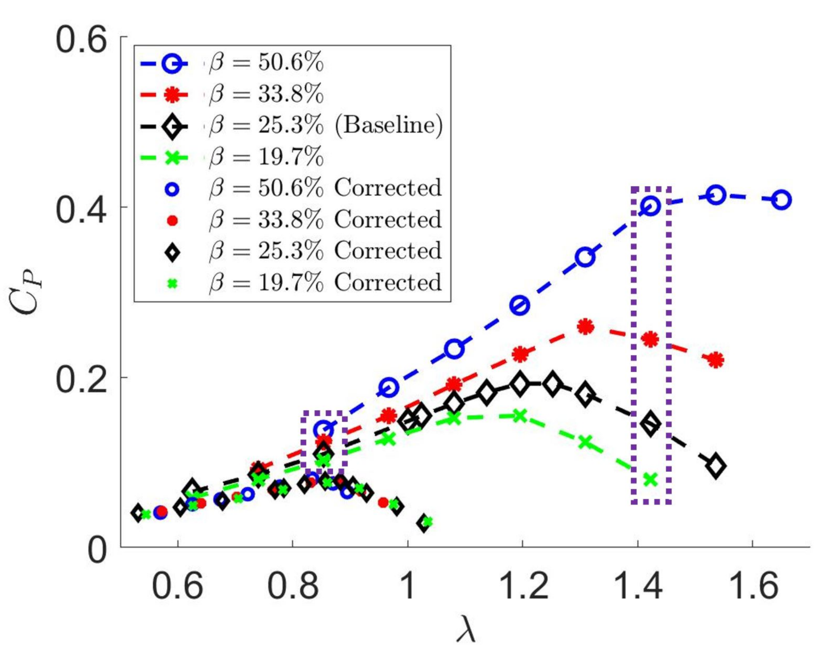
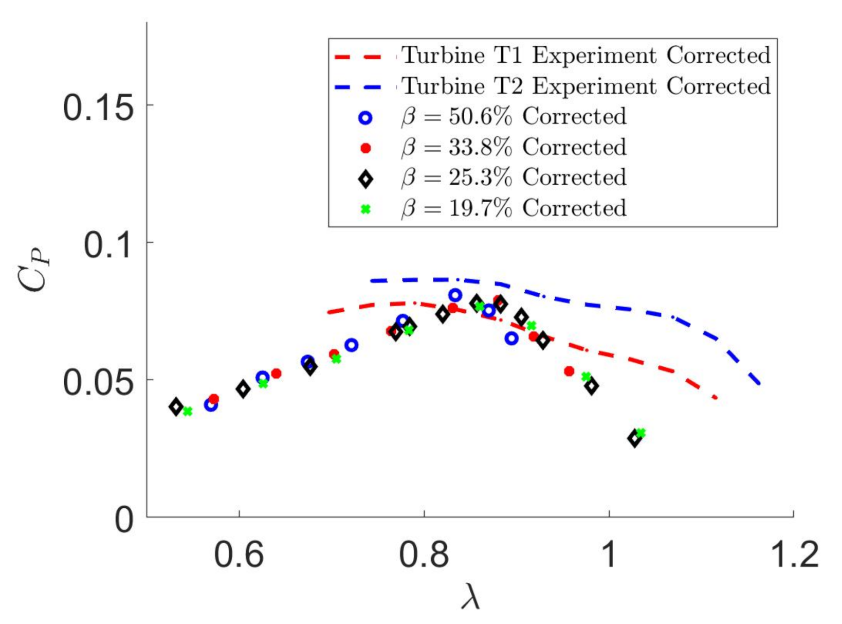
2.3.1. Comparison with Experimental Results
2.3.2. The Laboratory Frame of Reference
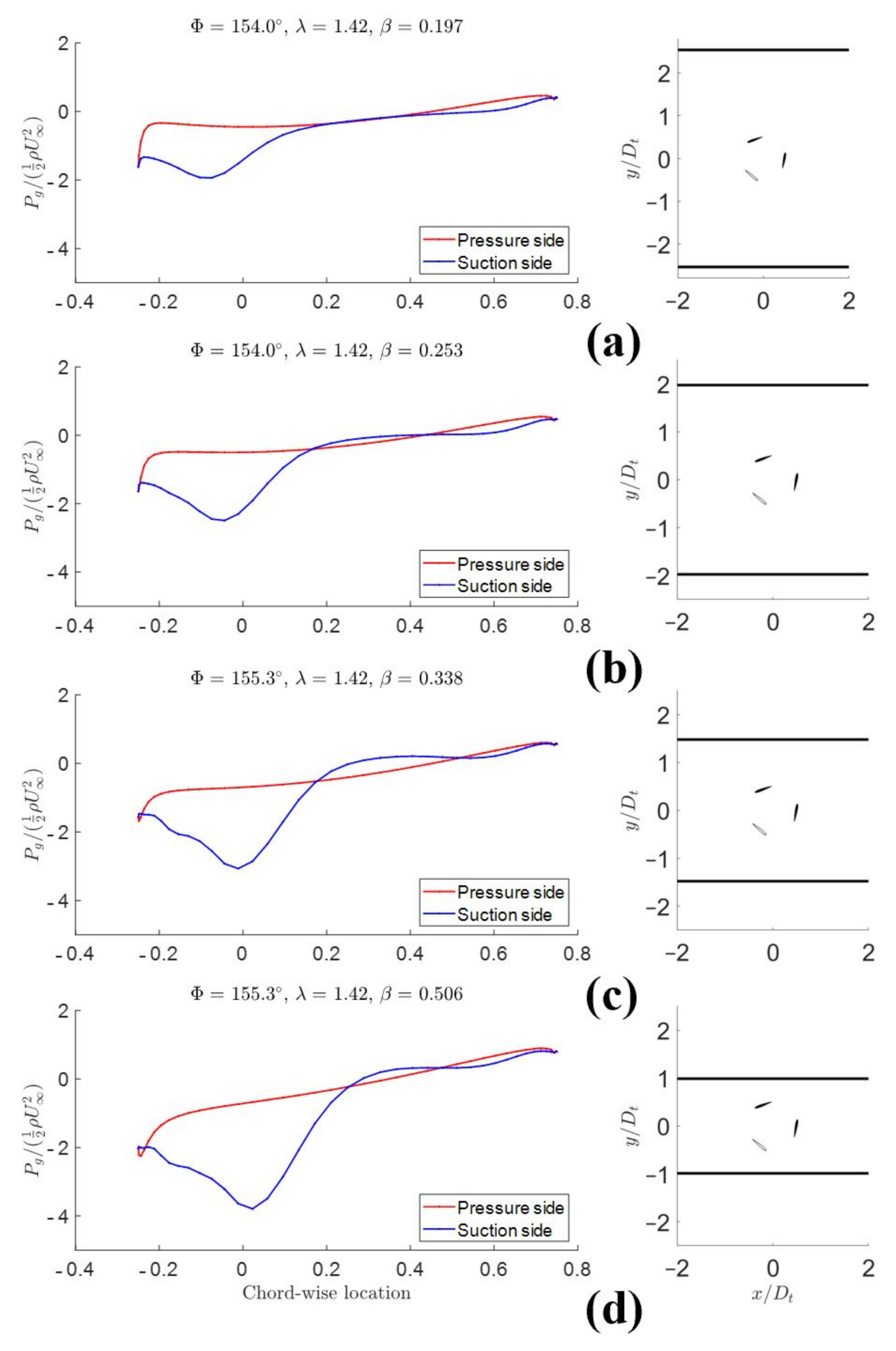
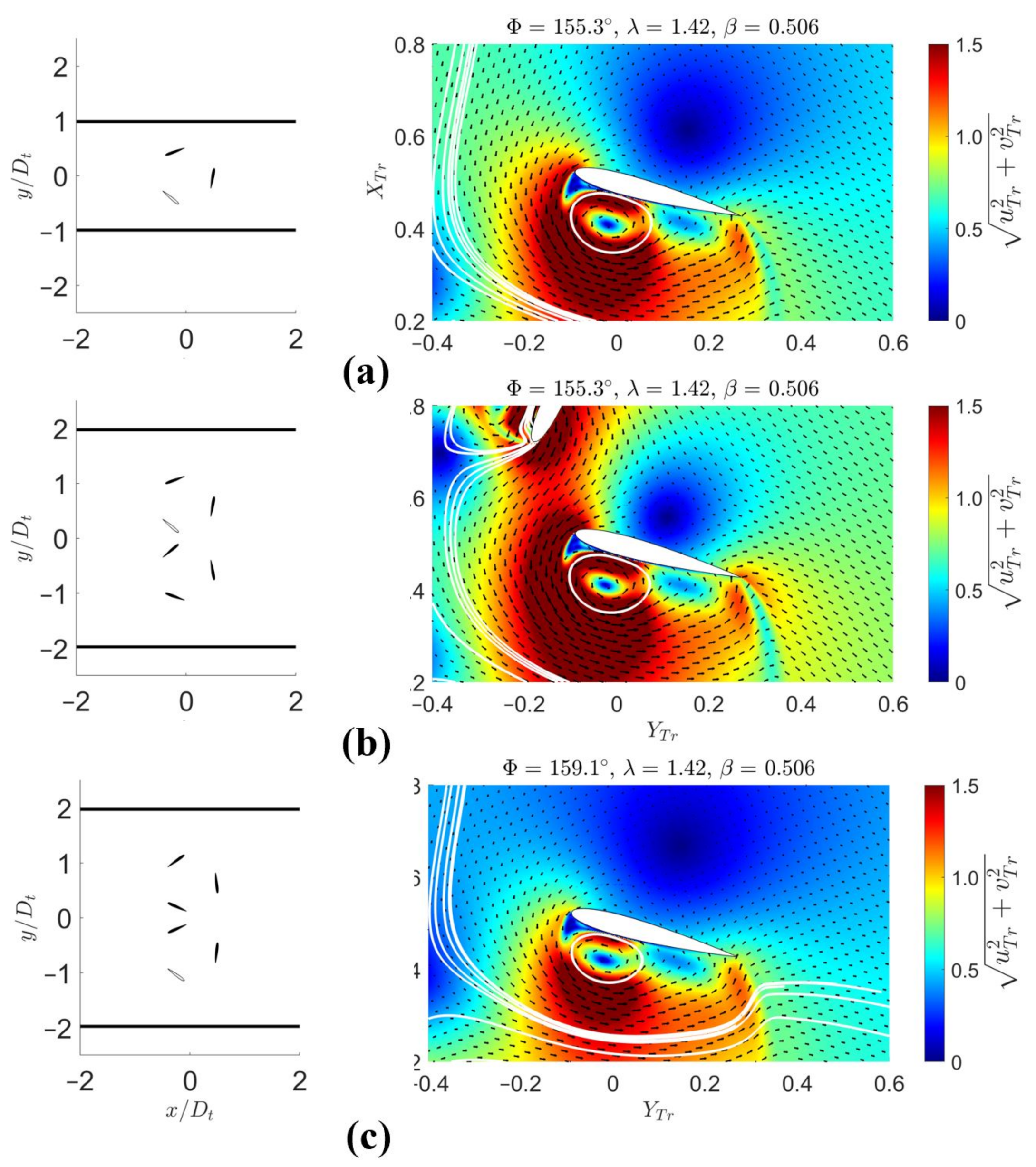
2.3.3. The Blade Frame of Reference
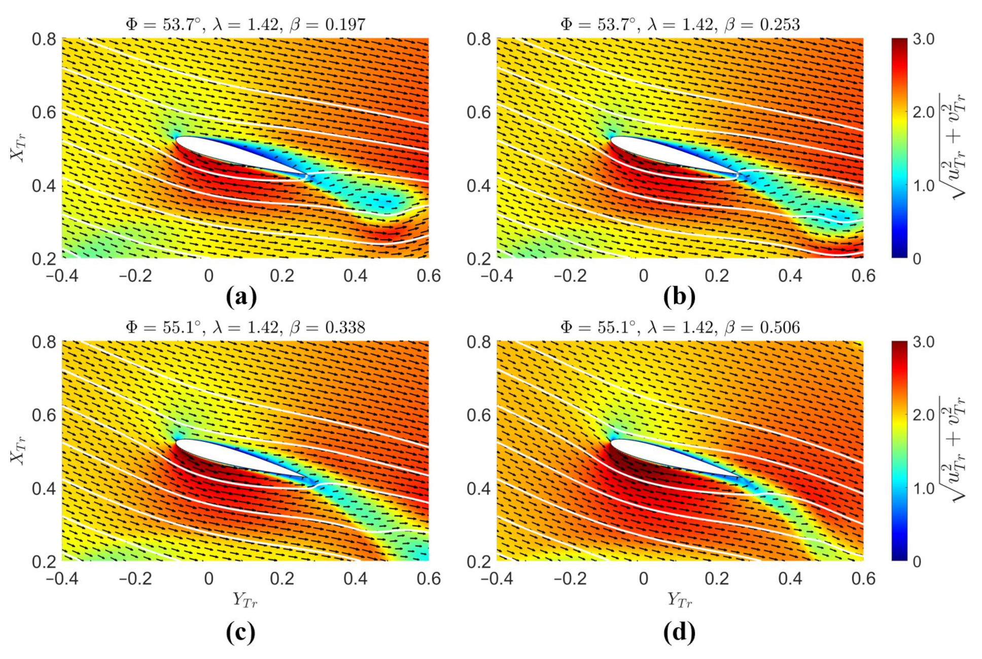
- (1)
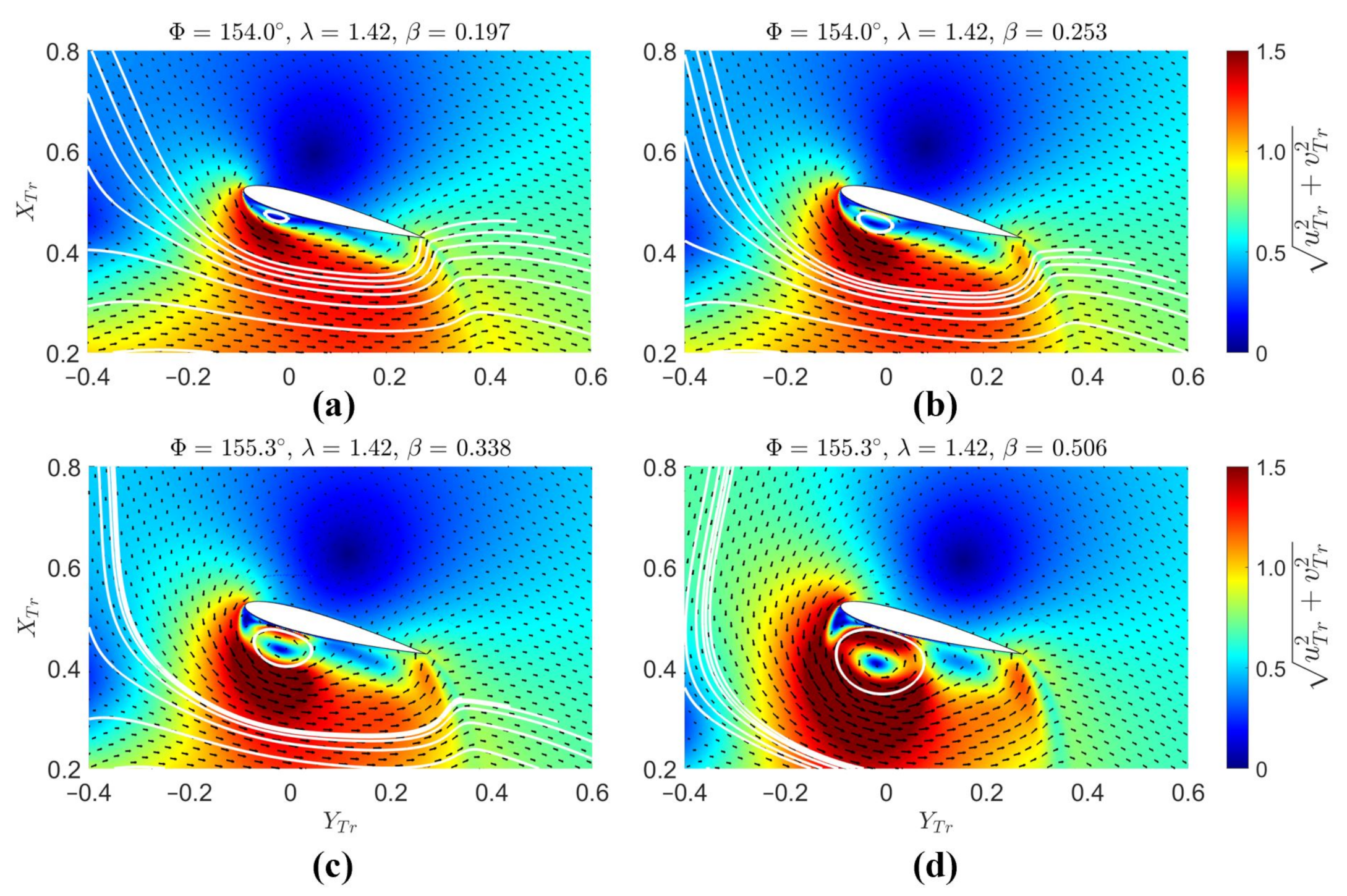
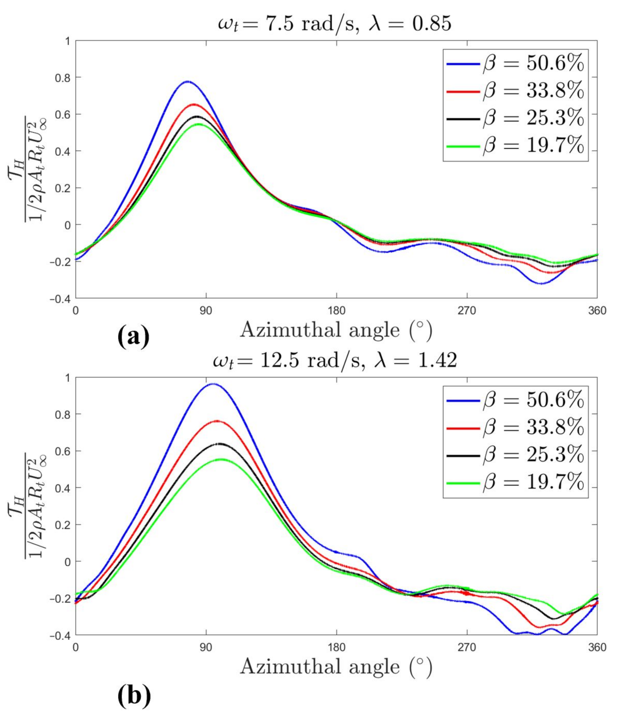
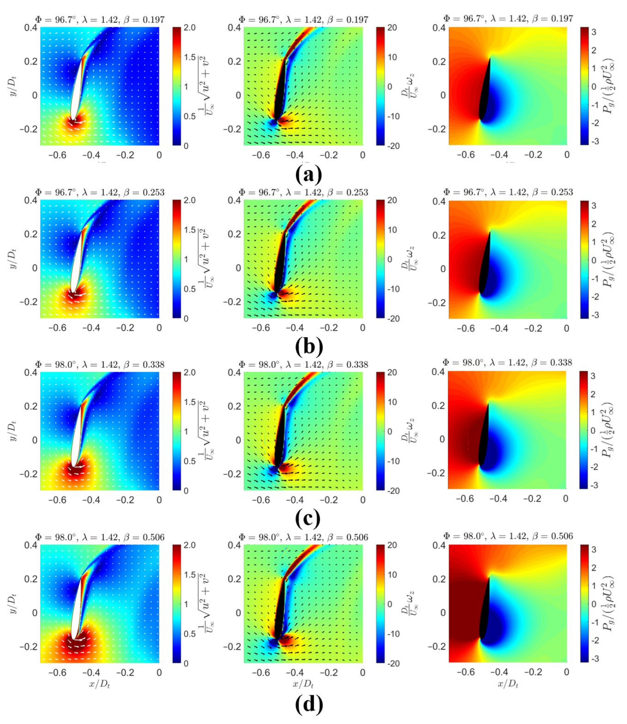
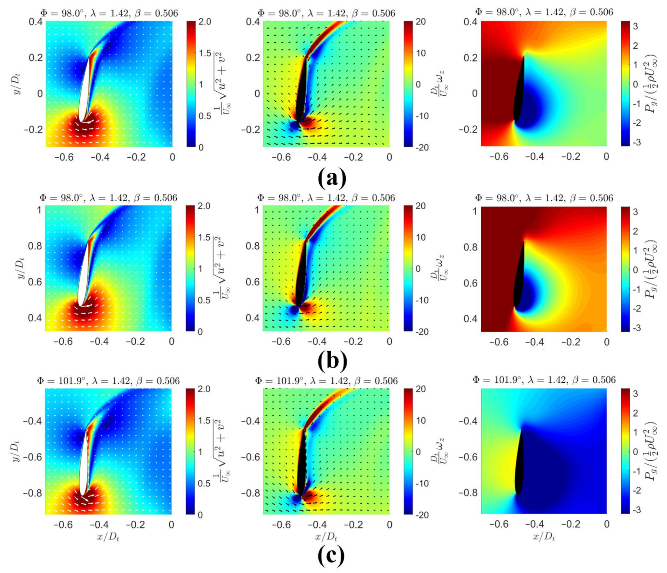
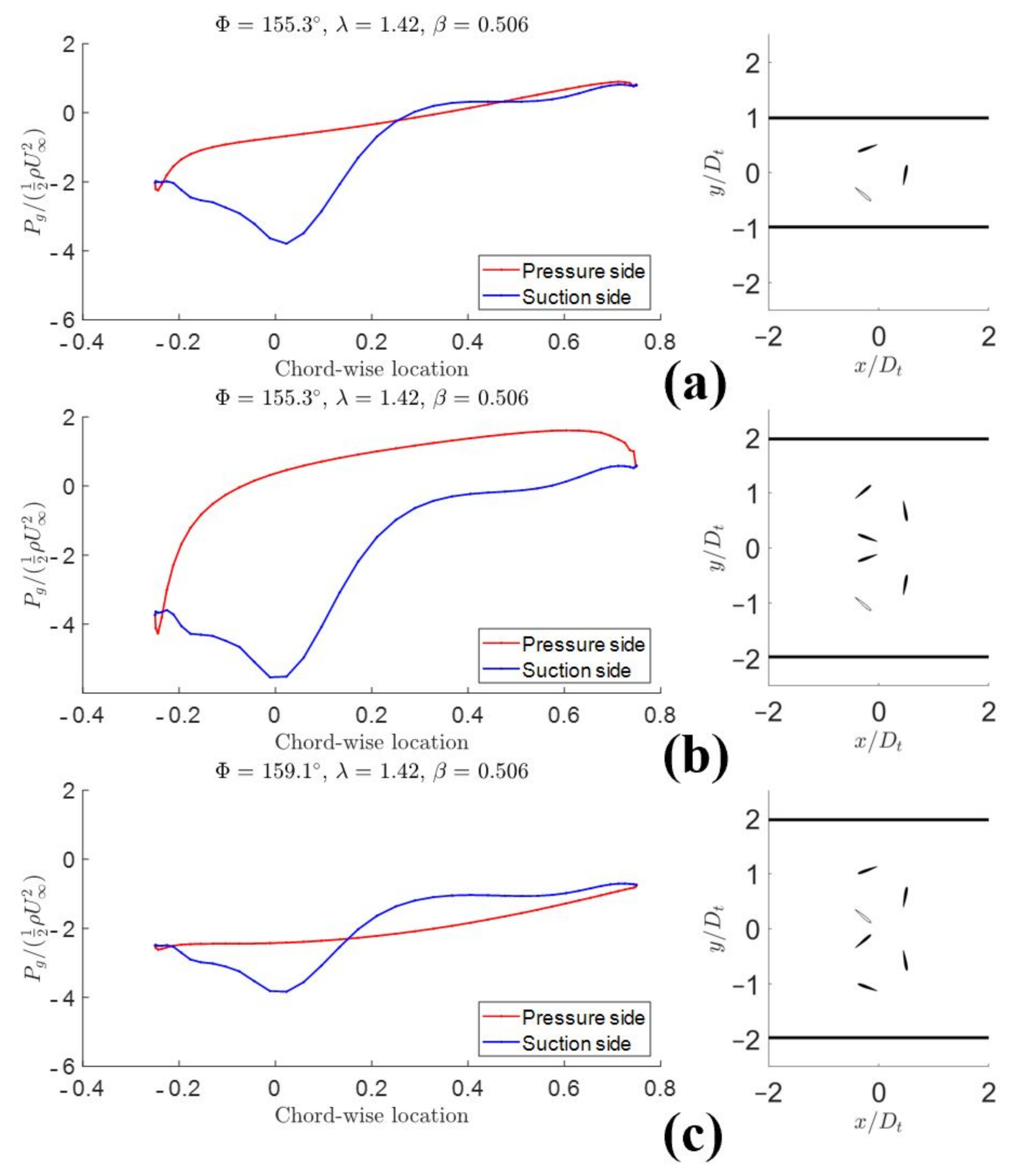
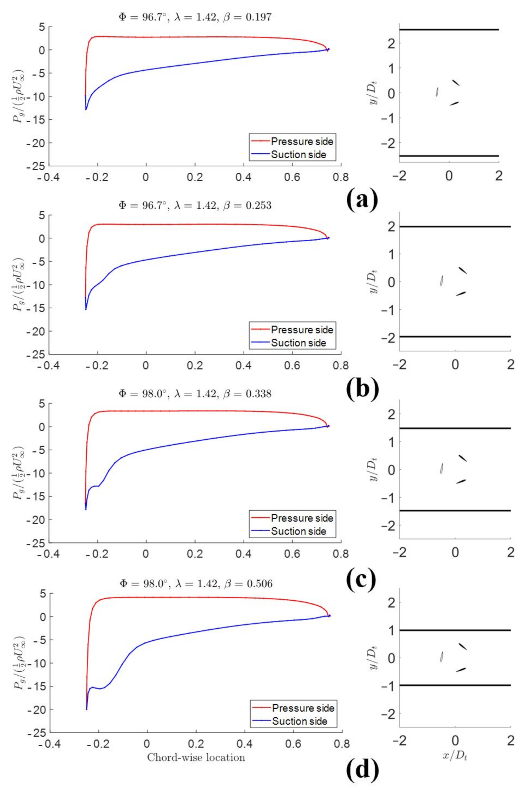
- Before the maximum point, the torque generation was due the attached fast flow on the inner of the blade, which created an associated low pressure region and suction force. As the azimuthal angle increased, the relative angle between the incoming flow and the blade chord also increased and resulted in higher lift and torque. Higher blockage ratio created faster flow on the suction side and smaller area of the blade wake.
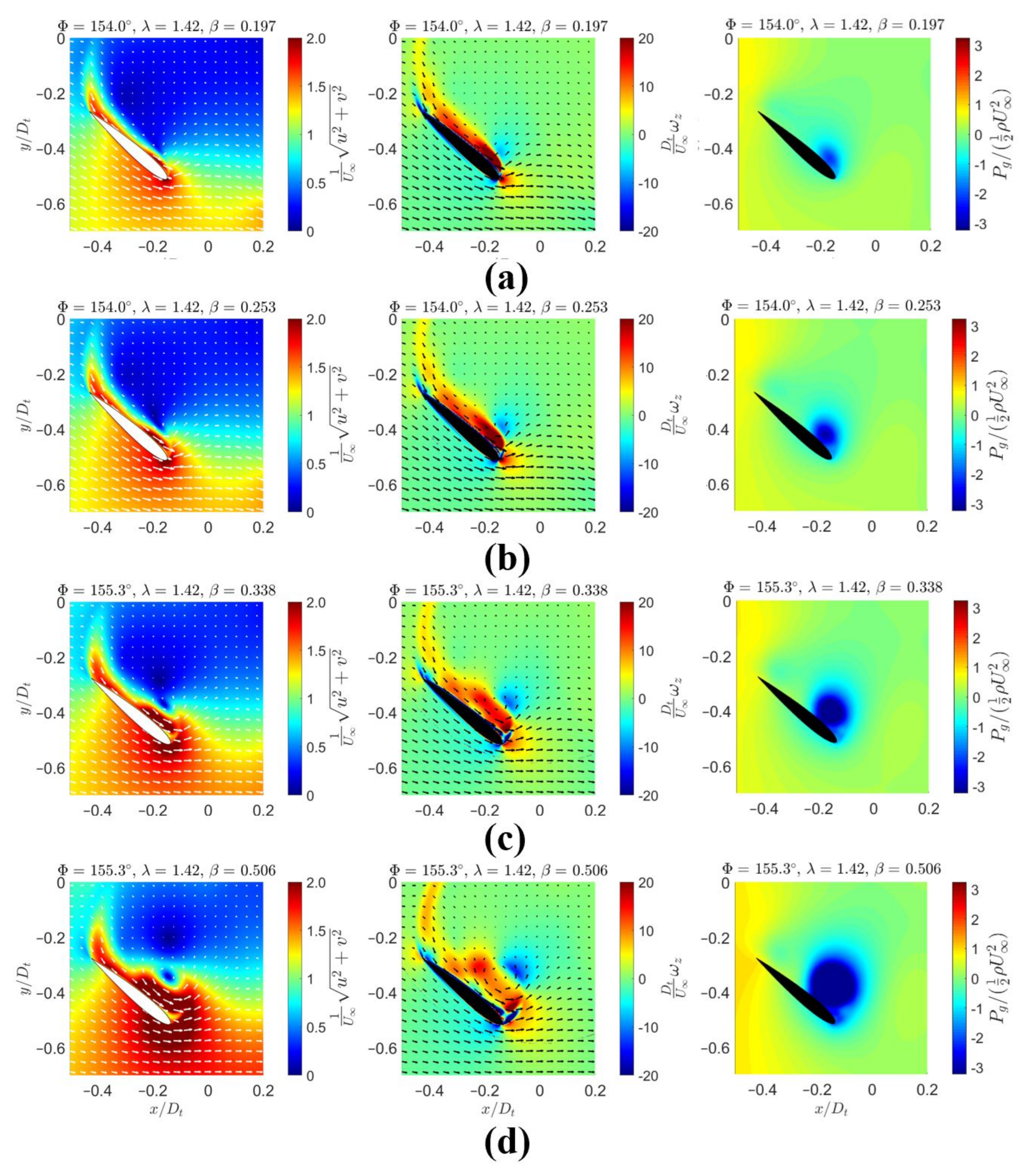
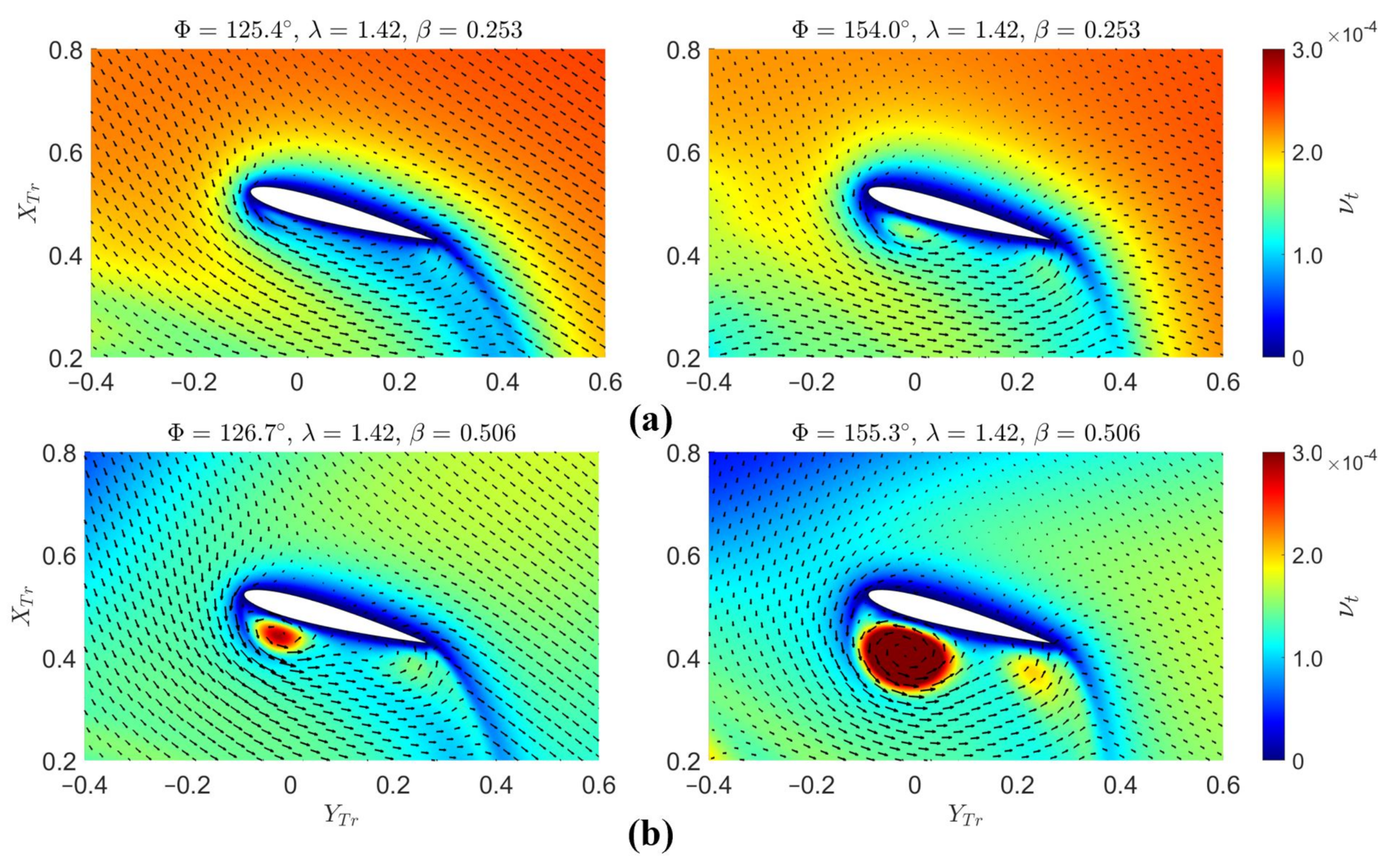
- (2)
- After reaching the maximum torque, the blade experienced the dynamic stall effect and the lift force was maintained by a vortex shed from the leading edge and attached on the suction side. Higher blockage ratio created a bigger and stronger vortex, which maintained higher lift and torque.

3. Twin Turbine Configurations
3.1. Materials and Methodology
3.1.1. System Geometry
3.1.2. Simulation Setup
3.2. Results and Discussion
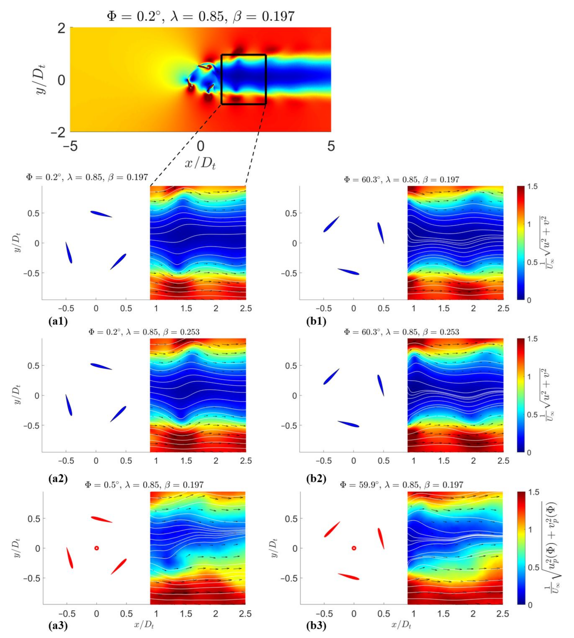
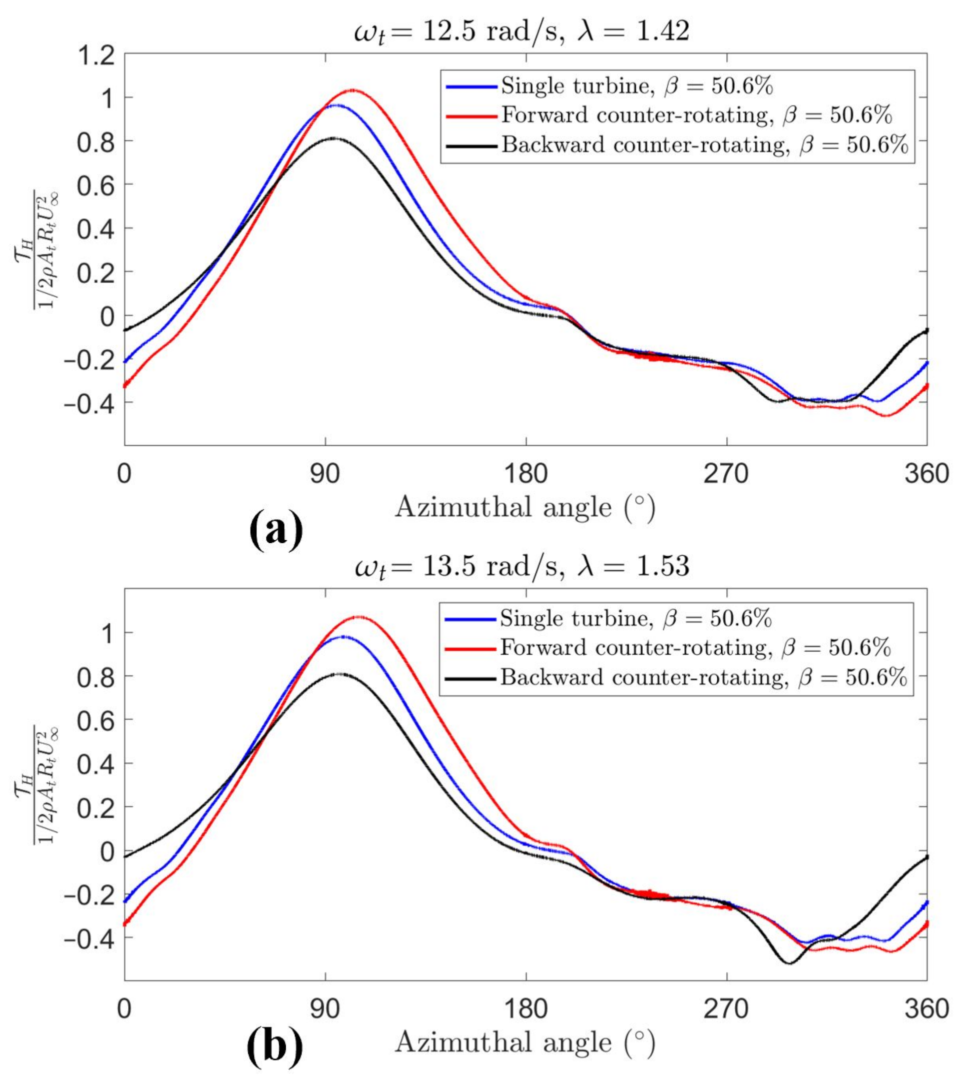
3.2.1. The Laboratory Frame of Reference
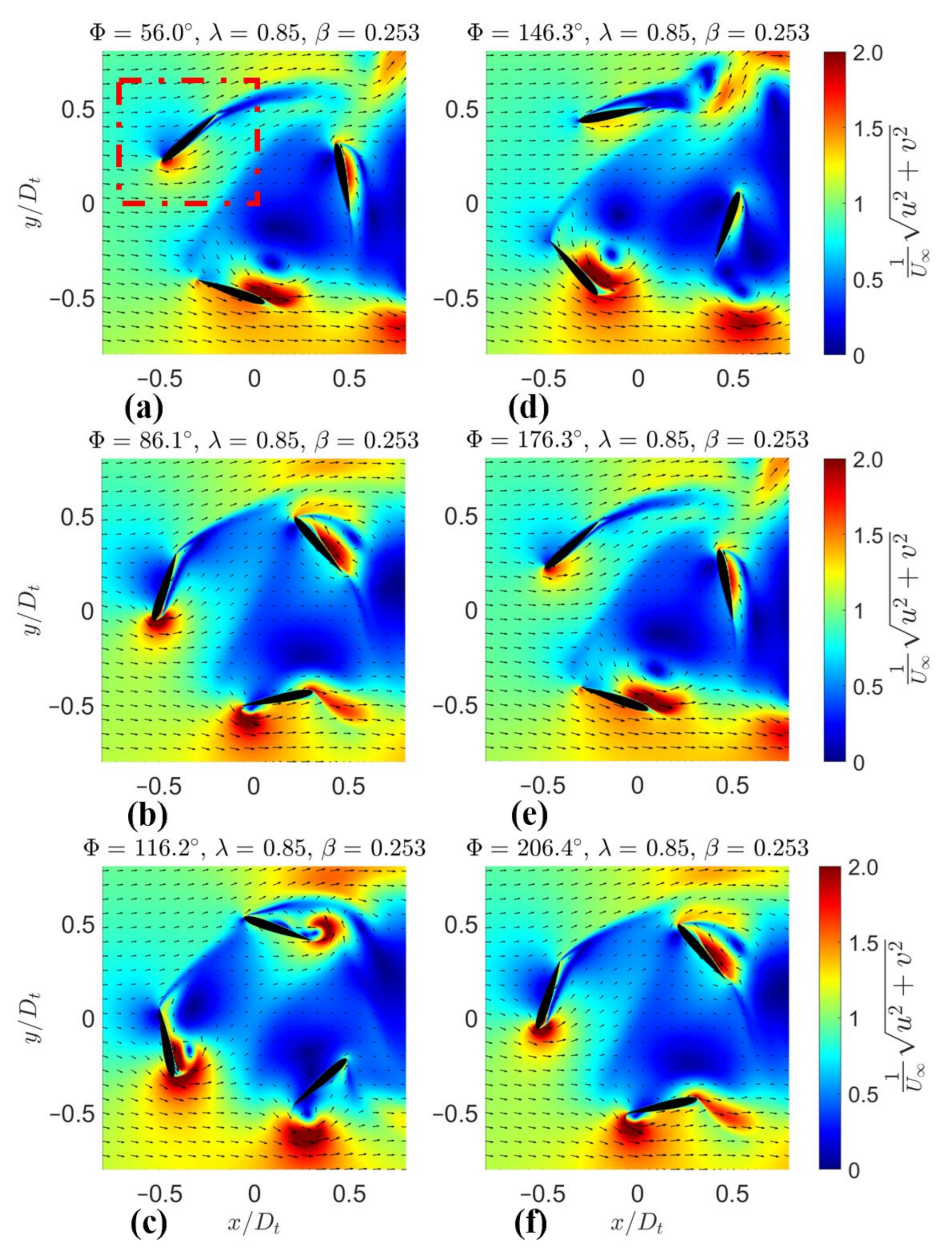
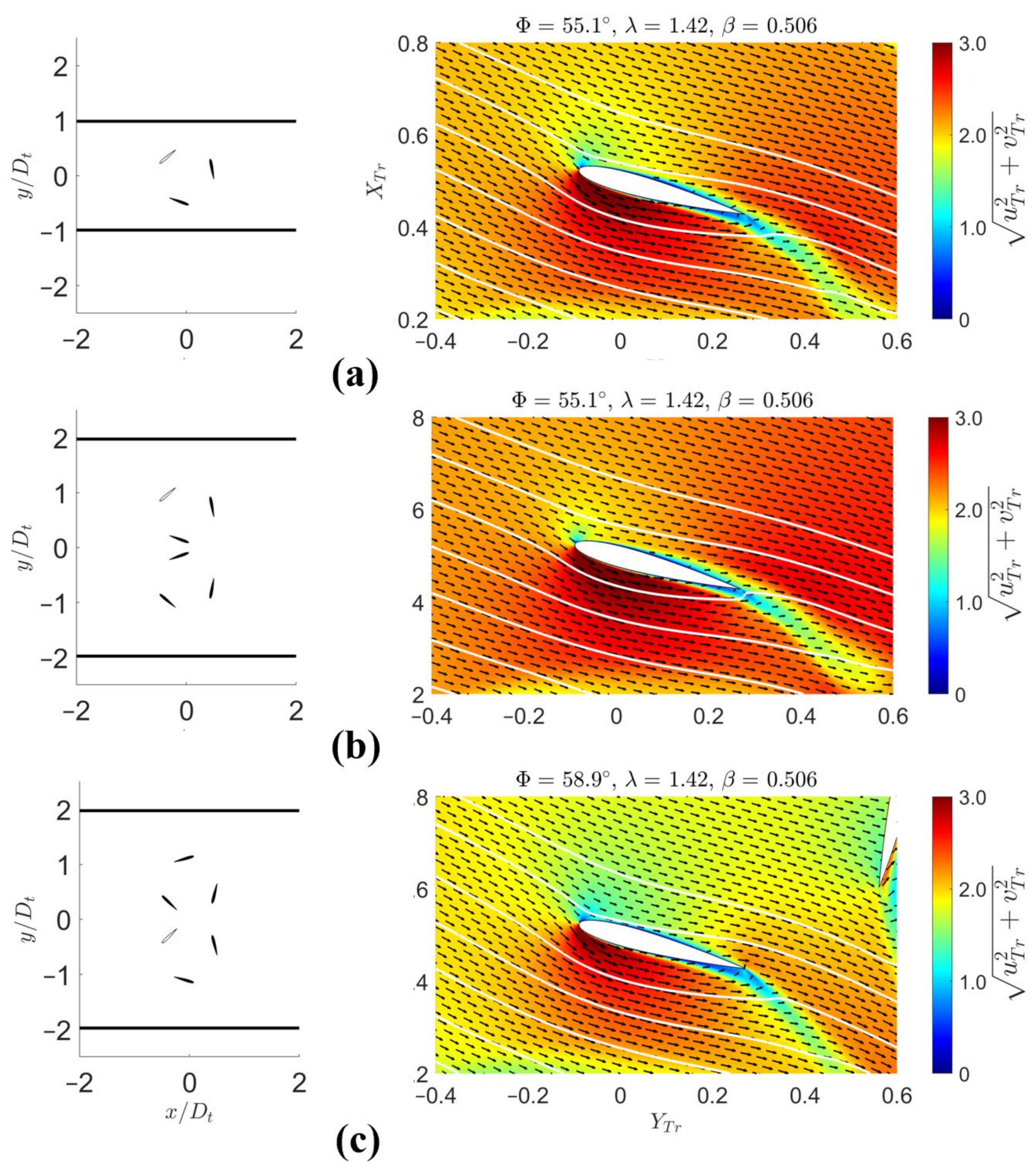
3.2.2. The Blade Frame of Reference
4. Summary and Conclusions
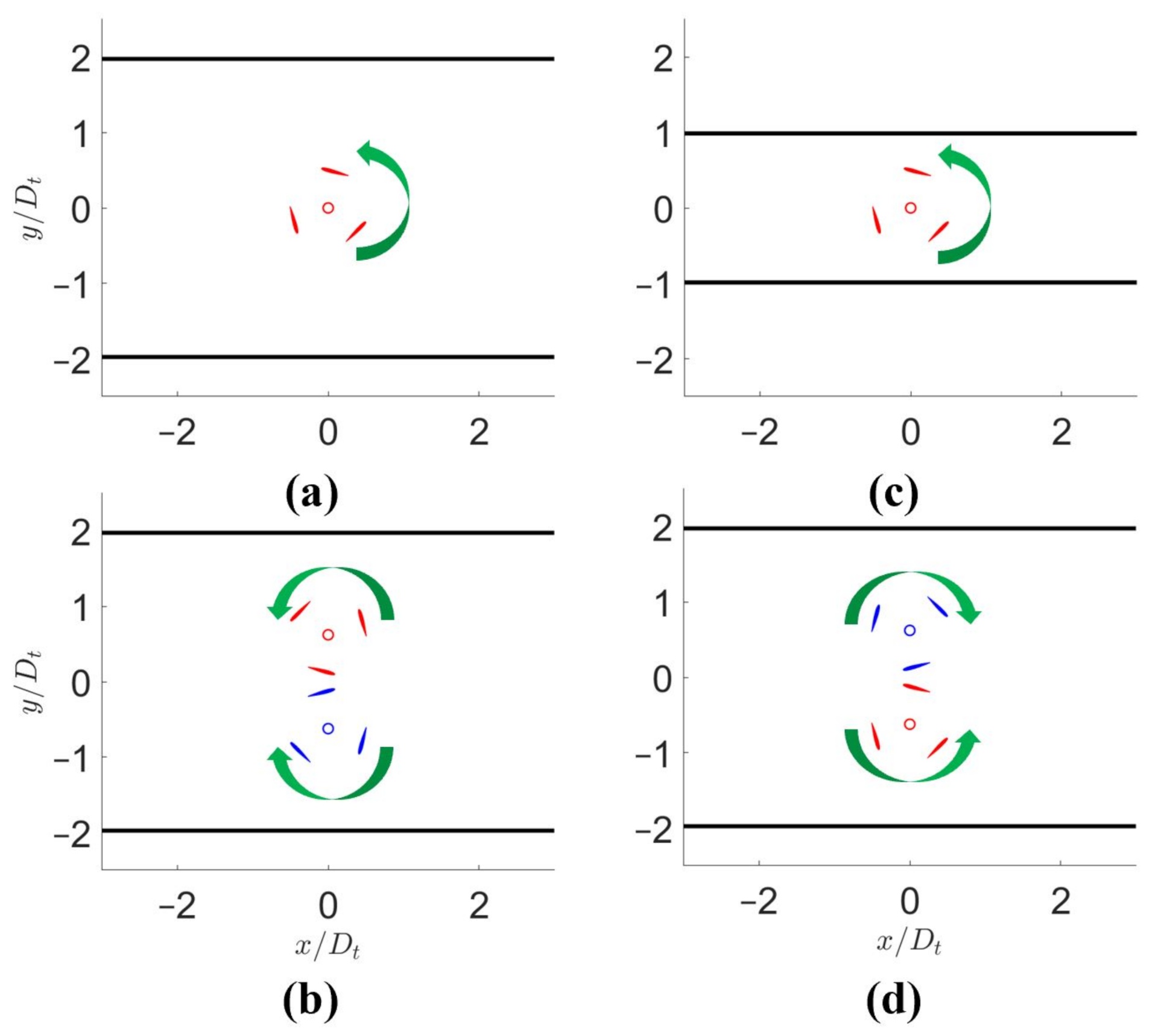
- (1)
- At the same blockage ratio, moving the turbine closer a fixed wall created positive impact on the positive torque phase.
- (2)
- Placing a moving object near the turbine could have both positive and negative impact depending on the movement direction of the object. Specifically, another turbine blade moving against the incoming freestream flow would have reduced the torque while movement in the same direction of the freestream created a stronger and bigger LEV to maintain higher hydrodynamic torque.
Author Contributions
Funding
Institutional Review Board Statement
Informed Consent Statement
Data Availability Statement
Acknowledgments
Conflicts of Interest
Abbreviations
| MHK | Marine hydrokinetic turbine; |
| VAWT | Vertical axis wind turbine; |
| PIV | Particle image velocimetry; |
| CFD | Computational fluid dynamics. |
References
- Consul, C.A.; Willden, R.H.J.; McIntosh, S.C. Blockage effects on the hydrodynamic performance of a marine cross-flow turbine. Philos. Trans. R. Soc. A Math. Phys. Eng. Sci. 2013, 371, 20120299. [Google Scholar] [CrossRef] [PubMed]
- Goude, A.; Agren, O. Simulations of a vertical axis turbine in a channel. Renew. Energy 2014, 63, 477–485. [Google Scholar] [CrossRef]
- Dossena, V.; Persico, G.; Paradiso, B.; Battisti, L.; Dell’Anna, S.; Brighenti, A.; Benini, E. An Experimental Study of the Aerodynamics and Performance of a Vertical Axis Wind Turbine in a Confined and Unconfined Environment. J. Energy Resour. Technol. 2014, 137, 051207. [Google Scholar] [CrossRef]
- Sarlak, H.; Nishino, T.; Martinez-Tossas, L.; Meneveau, C.; Sorensen, J. Assessment of blockage effects on the wake characteristics and power of wind turbines. Renew. Energy 2016, 93, 340–352. [Google Scholar] [CrossRef] [Green Version]
- Ross, H.; Polagye, B. An experimental assessment of analytical blockage corrections for turbines. Renew. Energy 2020, 152, 1328–1341. [Google Scholar] [CrossRef] [Green Version]
- Corke, T.C.; Thomas, F.O. Dynamic Stall in Pitching Airfoils: Aerodynamic Damping and Compressibility Effects. Annu. Rev. Fluid Mech. 2015, 47, 479–505. [Google Scholar] [CrossRef]
- Guillaud, N.; Balarac, G.; Goncalves, E. Large Eddy Simulations on a pitching airfoil: Analysis of the reduced frequency influence. Comput. Fluids 2018, 161, 1–13. [Google Scholar] [CrossRef] [Green Version]
- Wang, S.; Ingham, D.B.; Ma, L.; Pourkashanian, M.; Tao, Z. Numerical investigations on dynamic stall of low Reynolds number flow around oscillating airfoils. Comput. Fluids 2010, 39, 1529–1541. [Google Scholar] [CrossRef]
- Tsai, H.C. Numerical Investigation of Vertical-Axis Wind Turbines at Low Reynolds Number. Ph.D. Thesis, California Institute of Technology, Pasadena, CA, USA, 2016. [Google Scholar]
- Guillaud, N.; Balarac, G.; Goncalves, E.; Zanette, J. Large Eddy Simulations on Vertical Axis Hydrokinetic Turbines and flow phenomena analysis. IOP Conf. Ser. Earth Environ. Sci. 2016, 49, 102010. [Google Scholar] [CrossRef] [Green Version]
- Guilbot, M.; Barre, S.; Balarac, G.; Bonamy, C.; Guillaud, N. A numerical study of Vertical Axis Wind Turbine Performances in Twin-Rotor Configurations. J. Phys. Conf. Ser. 2020, 1618, 052012. [Google Scholar] [CrossRef]
- Dabiri, J. Potential order-of-magnitude enhancement of wind farm power density via counter-rotating vertical-axis wind turbine arrays. J. Renew. Sustain. Energy 2011, 3, 043104. [Google Scholar] [CrossRef] [Green Version]
- Brownstein, I.D.; Wei, N.J.; Dabiri, J.O. Aerodynamically Interacting Vertical-Axis Wind Turbines: Performance Enhancement and Three-Dimensional Flow. Energies 2019, 12, 2724. [Google Scholar] [CrossRef] [Green Version]
- Jiang, Y.; Zhao, P.; Stoesser, T.; Wang, K.; Zhou, L. Experimental and numerical investigation of twin vertical axis wind turbines with a deflector. Energy Convers. Manag. 2020, 209, 112588. [Google Scholar] [CrossRef]
- Doan, M.; Kai, Y.; Obi, S. Twin Marine Hydrokinetic Cross-Flow Turbines in Counter Rotating Configurations: A Laboratory-Scaled Apparatus for Power Measurement. J. Mar. Sci. Eng. 2020, 8, 918. [Google Scholar] [CrossRef]
- Doan, M.; Kai, Y.; Takuya, K.; Obi, S. Flow Field Measurement of Laboratory-Scaled Cross-Flow Hydrokinetic Turbines: Part 1—The Near-Wake of a Single Turbine. J. Mar. Sci. Eng. 2021, 9, 489. [Google Scholar]
- Doan, M.; Takuya, K.; Obi, S. Flow Field Measurement of Laboratory-Scaled Cross-Flow Hydrokinetic Turbines: Part 2—The Near-Wake of Twin Turbines in Counter-Rotating Configurations. J. Mar. Sci. Eng. 2021, 9, 777. [Google Scholar]
- Bachant, P.; Wosnik, M. Modeling the near-wake of a vertical-axis cross-flow turbine with 2-D and 3-D RANS. J. Renew. Sustain. Energy 2016, 8, 053311. [Google Scholar] [CrossRef] [Green Version]
- The OpenFOAM Foundation. OpenFOAM 4.1. Available online: https://openfoam.org/version/4-1/ (accessed on 1 July 2021).
- Doan, M.N.; Alayeto, I.H.; Padricelli, C.; Obi, S.; Totsuka, Y. Experimental and computational fluid dynamic analysis of laboratory-scaled counter-rotating cross-flow turbines in marine environment. In Proceedings of the ASME 2018 5th Joint US-European Fluids Engineering Division Summer Meeting, Montreal, QC, Canada, 15 July 2018; American Society of Mechanical Engineer: New York, NY, USA, 2018; Volume 2, p. V002T14A003. [Google Scholar]
- Doan, M.N.; Alayeto, I.H.; Kumazawa, K.; Obi, S. Computational fluid dynamic analysis of a marine hydrokinetic crossflow turbine in low Reynolds number flow. In Proceedings of the ASME-JSME-KSME 2019 8th Joint Fluids Engineering Conference, San Francisco, CA, USA, 28 July–1 August 2019; American Society of Mechanical Engineer: New York, NY, USA, 2019; Volume 2, p. V002T02A067. [Google Scholar]
- Alayeto, I.H.; Doan, M.N.; Kumazawa, K.; Obi, S. Wake characteristics comparison between isolated and pair configurations of marine hydrokinetic crossflow turbines at low Reynolds numbers. In Proceedings of the ASME-JSME-KSME 2019 8th Joint Fluids Engineering Conference, San Francisco, CA, USA, 28 July–1 August 2019; American Society of Mechanical Engineer: New York, NY, USA, 2019; Volume 1, p. V001T01A037. [Google Scholar]
- Rezaeiha, A.; Montazeriab, H.; Blockenab, B. On the accuracy of turbulence models for CFD simulations of vertical axis wind turbines. Energy 2019, 180, 838–857. [Google Scholar] [CrossRef]
- Spalart, P.; Allmaras, S. A one-equation turbulence model for aerodynamic flows. Rech. Aerosp. 1992, 1, 5–12. [Google Scholar]
- Balduzzi, F.; Bianchini, A.; Maleci, R.; Ferrara, G.; Ferrari, L. Critical issues in the CFD simulation of Darrieus wind turbines. Renew. Energy 2016, 85, 419–435. [Google Scholar] [CrossRef]
- Bianchini, A.; Balduzzi, F.; Bachant, P.; Ferrara, G.; Ferrari, L. Effectiveness of two-dimensional CFD simulations for Darrieus VAWTs: A combined numerical and experimental assessment. Energy Convers. Manag. 2017, 136, 318–328. [Google Scholar] [CrossRef]
- Bahaja, A.; Molland, A.; Chaplin, J.; Battena, W. Power and thrust measurements of marine current turbines under various hydrodynamic flow conditions in a cavitation tunnel and a towing tank. Renew. Energy 2007, 32, 407–426. [Google Scholar] [CrossRef]
- Kinsey, T.; Dumas, G. Impact of channel blockage on the performance of axial and cross-flow hydrokinetic turbines. Renew. Energy 2007, 103, 239–254. [Google Scholar] [CrossRef]
- Adhikari, R.C.; Vaz, J.; Wood, D. Cavitation Inception in Crossflow Hydro Turbines. Energies 2016, 9, 237. [Google Scholar] [CrossRef] [Green Version]
- Da Silva, P.A.S.F.; Shinomiya, L.D.; de Oliveira, T.F.; Vaz, J.R.P.; Mesquita, A.L.A.; Junior, A.C.P.B. Design of Hydrokinetic Turbine Blades Considering Cavitation. Energy Procedia 2015, 75, 277–282. [Google Scholar] [CrossRef] [Green Version]


| Parameter | Symbol | Value (Unit) |
|---|---|---|
| Blade chord | c | 2.54 (cm) |
| Solidity | 0.39 (-) | |
| Reynolds number (diameter based) | 20,000 (-) | |
| Water density | 998 (kg/m) | |
| Freestream velocity | 0.3 (m/s) | |
| Blockage ratio | 0.197/0.253/0.338/0.506 (-) |
| Case | Total Number of Cells | ||
|---|---|---|---|
| 1 | 222 | 30 | 588,649 |
| 2 | 296 | 40 | 1,026,883 |
| 3 | 333 | 45 | 1,304,364 |
| 4 | 370 | 50 | 1,605,068 |
| 5 | 444 | 60 | 2,305,123 |
| Case | Note | |
|---|---|---|
| T1 Experiment | 19.7% | —Optimal power output |
| Numerical Model 1 | 19.7% | Same blockage ratio as the experiment |
| Numerical Model 2 | 25.3% | Same physical dimensions as the experiment |
| Case | Difference from the Baseline | ||
|---|---|---|---|
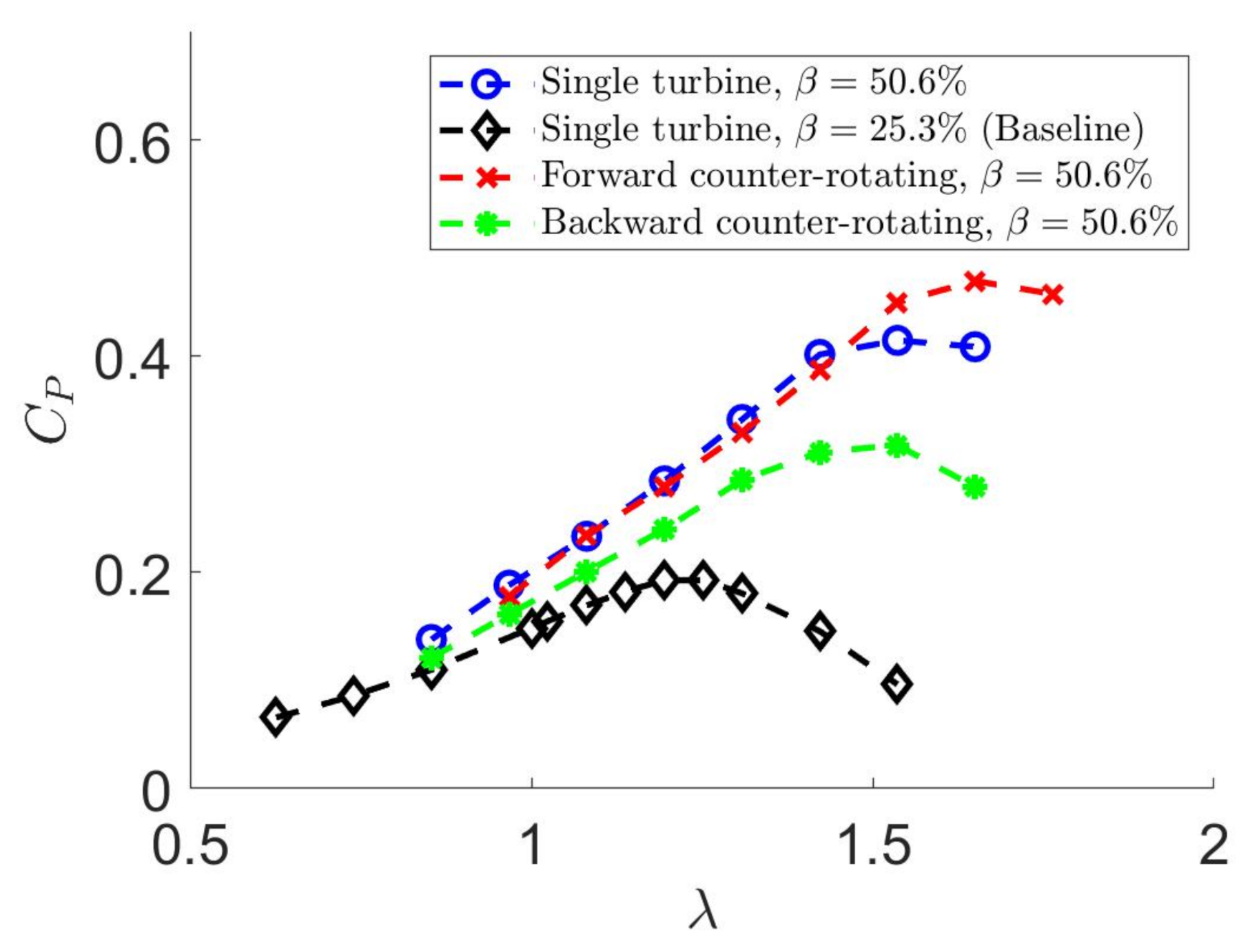
| Single turbine, (baseline) | 1.25 | 0.19 | N/A |
| Single turbine, | 1.53 | 0.41 | 115% |
| Forward counter-rotating | 1.65 | 0.47 | 144% |
| Backward counter-rotating | 1.53 | 0.32 | 65.7% |
Publisher’s Note: MDPI stays neutral with regard to jurisdictional claims in published maps and institutional affiliations. |
© 2021 by the authors. Licensee MDPI, Basel, Switzerland. This article is an open access article distributed under the terms and conditions of the Creative Commons Attribution (CC BY) license (https://creativecommons.org/licenses/by/4.0/).
Share and Cite
Doan, M.N.; Obi, S. Numerical Study of the Dynamic Stall Effect on a Pair of Cross-Flow Hydrokinetic Turbines and Associated Torque Enhancement Due to Flow Blockage. J. Mar. Sci. Eng. 2021, 9, 829. https://doi.org/10.3390/jmse9080829
Doan MN, Obi S. Numerical Study of the Dynamic Stall Effect on a Pair of Cross-Flow Hydrokinetic Turbines and Associated Torque Enhancement Due to Flow Blockage. Journal of Marine Science and Engineering. 2021; 9(8):829. https://doi.org/10.3390/jmse9080829
Chicago/Turabian StyleDoan, Minh N., and Shinnosuke Obi. 2021. "Numerical Study of the Dynamic Stall Effect on a Pair of Cross-Flow Hydrokinetic Turbines and Associated Torque Enhancement Due to Flow Blockage" Journal of Marine Science and Engineering 9, no. 8: 829. https://doi.org/10.3390/jmse9080829
APA StyleDoan, M. N., & Obi, S. (2021). Numerical Study of the Dynamic Stall Effect on a Pair of Cross-Flow Hydrokinetic Turbines and Associated Torque Enhancement Due to Flow Blockage. Journal of Marine Science and Engineering, 9(8), 829. https://doi.org/10.3390/jmse9080829