Inversion of Initial Field Based on a Temperature Transport Adjoint

Abstract

The setting of initial values is one of the key problems in ocean numerical prediction, with the accuracy of sea water temperature (SWT) simulation and prediction greatly affected by the initial field quality. In this paper, we describe the development of an adjoint assimilation model of temperature transport used to invert the initial temperature field by assimilating the observed data of sea surface temperature (SST) and vertical temperature. Two ideal experiments were conducted to verify the feasibility and validity of this method. By assimilating the “observed data”, the mean absolute error (MAE) between the simulated temperature data and the “observed data” decreased from 1.74 °C and 1.87 °C to 0.13 °C and 0.14 °C, respectively. The spatial distribution of SST difference and the comparison of vertical data also indicate that the regional error of vertical data assimilation is smaller. In the practical experiment, the monthly average temperature field provided by World Ocean Atlas 2018 was selected as background filed and optimized by assimilating the SST data and Argo vertical temperature observation data, to invert the temperature field at 0 a.m. on 1 December 2014 in the South China Sea. Through data assimilation, MAE was reduced from 1.29 °C to 0.65 °C. In terms of vertical observations data comparison and SST spatial distribution, the temperature field obtained by inversion is in good agreement with SST and Argo observations.

1. Introduction

As one of the few semi-closed deep-sea basins, the South China Sea (SCS) which is located in the southeast of Asia, is a sensitive area of air-sea interaction. Sea water temperature (SWT) is an important parameter of the state of ocean thermodynamic, which plays a key role in ocean circulation, atmospheric circulation, and air-sea interaction. Sea surface temperature (SST) is a key indicator of global climate change [1,2], as a major driving force of global climate, the response of tropical SST to global warming is important [3,4]. It directly affects the exchange of heat, momentum, and water vapor between the atmosphere and the ocean, and is an important parameter driving the global circulation, which is related to the global energy equilibrium [5,6,7,8]. The importance of SWT research and prediction is self-evident; many scholars have performed numerous studies on the numerical simulation and prediction of SST in offshore China [7,8,9,10,11].

With the improvement of the model and computer technology, the resolution and accuracy of global ocean numerical simulation are also optimized [12,13,14], but there are still some errors in the forecast results induced by the following issues. On the one hand, models have the problem of initial field uncertainty [15,16]. Unlike the prediction of storm surges and waves, the prediction of sea temperature seriously depends on the initial values. Thus, the improvement of the quality of the initial values is increasingly important. As early as the 1940s, Kolmogorov [17] pointed out that small initial errors can cause significant differences in fluid states. In order to improve the accuracy of SST prediction, the quality of the initial SST field should first be improved [18]. Peng and Xie [15] pointed out that initial conditions is one of the main sources of model error or uncertainties. Zhang et al. [19] also attributed some model deficiencies to errors in model initial conditions. How to obtain a more reasonable and accurate initial field is a key issue in ocean numerical simulation and forecast. On the other hand, numerical models cannot fully describe various physical processes in the ocean [20,21]. SWT variation is not only affected by convection and diffusion factors, but also highly correlated with sensible heat flux (SHF), latent heat flux (LHF) and solar radiation. In order to accurately simulate and forecast the SWT, the influence of the sea surface solar radiation and penetration radiation should be applied in the models [22].

With the development of remote sensing technology, various remote sensing instruments provide data with wide coverage and high spatial-temporal resolution for ocean monitoring. However, the information obtained is merely limited to the sea surface. The Argo (Array for Real-time Geostrophic Oceanography) project, launched in the 1990s, established a global real-time ocean observation data system to sample the ocean from surface down to 2000 dbar, and provided three-dimensional (3D) thermohaline data with global coverage [23]. Hosoda et al. [24] used the optimal interpolation (OI) method to construct a dataset of global monthly average temperature based on Argo float data and other observation data. Through distribution of observed points and interpolation error, it was proved to work well for global mapping. Zhou et al. [25] used Argo float data and SST data to reconstruct the 3D ocean temperature field, and an experiment was performed for the Pacific Ocean south of Japan. The reconstructed field achieved a satisfactory accuracy with a higher resolution, and more mesoscale information was found in the reconstructed field.

In order to maximize the use of observed data and reduce the error between the simulation and observation, the adjoint assimilation method is a suitable choice. The adjoint assimilation method takes the real problems to be solved as the conditional minimum problems. It is a method used to minimize the cost function which represents the error between simulation and observation data by taking equations, initial conditions, and boundary conditions as constraints [26]. Andreu-Burillo et al. [27] examined the ability of a one-dimensional SST assimilation scheme to improve the 3D structure of the temperature field in a shelf model, and proved that assimilation improved the error statistics of the modelled SST. Peng et al. [28] evaluated the role of a 4D-Var algorithm based on POM (Princeton Ocean Model) and its adjoint for storm surge simulation, by adjusting both the initial conditions and the upper boundary conditions, the storm surge simulation was improved. South China Sea Operational Oceanography Forecasting System (SCSOFS) was built to provide daily updated hydrodynamic forecasting in SCS for the future 5 days since 2013, and it also had been improved through comprehensive updates of the configurations of the physical model and data assimilation scheme [29].

In this paper, to achieve a better combination of data and model and make the simulation results more consistent with the actual temperature distribution, an adjoint assimilation model of temperature transport is established to invert the 3D initial temperature field by assimilating the satellite SST observation and the Argo observation, which provides higher quality initial value for temperature simulation and prediction.

2. Models and Method

2.1. Forward Model

According to the convection and diffusion process of and taking solar radiation and sea surface heat fluxes factors into consideration, the temperature transport equation can be expressed as:

$$\begin{array}{c}\frac{\partial T}{\partial t}+u\frac{\partial T}{\partial x}+v\frac{\partial T}{\partial y}+w\frac{\partial T}{\partial z}=\\ \frac{\partial }{\partial x}\left(A_H\frac{\partial T}{\partial x}\right)+\frac{\partial }{\partial y}\left(A_H\frac{\partial T}{\partial y}\right)+\frac{\partial }{\partial z}\left(K_H\frac{\partial T}{\partial z}\right)+{\theta }_c \end{array}$$

(1)

where T represents the SWT; u, v and w are the flow velocity in x, y and z directions; $A_H$ and $K_H$ are the temperature diffusion coefficients in horizontal and vertical directions respectively; ${\theta }_c$ represents the heat fluxes term, which can be specifically expressed as:

$${\theta }_c=\{\begin{array}{rr}\frac{\left(1-r\right)Q_z-Q_l}{{\rho }_0{C}_p},& z=0\\ \frac{r{Q}_z{e}^{-\frac{z}{h_r}}}{{\rho }_0{C}_{p}z},& z>0\end{array}$$

(2)

$Q_z$ is the net solar shortwave radiation reaching the sea surface; $Q_l$ is the heat loss from the sea surface due to long-wave radiation, SHF, and LHF. R is the separation coefficient, which represents the ratio of solar shortwave radiation energy into the deep ocean without being absorbed by the sea surface to the total solar radiation energy; $H_r$ is the e-fold scale of penetrating shortwave radiation attenuated with the depth of sea water [30,31]; $C_p$ is the specific heat capacity of seawater and ${\rho }_0$ is the density of sea water.

The open boundary condition is described as:

$$\begin{array}{c}\begin{array}{c}\frac{\partial T}{\partial t}=0,V_n\le 0\\ \\ \end{array}\\ \frac{\partial T}{\partial n}=0,V_n>0\end{array}$$

(3)

2.2. Adjoint Model

Adjoint assimilation method has been widely used in atmospheric and oceanic studies. Fan and Lv [32] used adjoint method to assimilate chlorophyll-a data from SeaWiFs through a simple NPZD model, which reproduced regional features of distribution, and the error was also smaller than that of traditional methods. Zhang et al. [33] used the adjoint method to optimize the bottom friction coefficient, which effectively improved the accuracy of regional tidal numerical simulation. Based on the marine ecological dynamics model, Wang et al. [34] studied the initial pollution filed in the Bohai Sea by adopting the adjoint method to assimilate monitoring data. Wang et al. [35] established a three-dimensional viscous sediment transport model with the adjoint assimilation method, and obtained good numerical simulation results. In addition, the adjoint assimilation method has also been applied in numerous other ecosystem dynamics and pollutant simulation studies [36,37,38,39].

The adjoint assimilation method based on Lagrange multiplier method is used to invert the temperature field in the SCS, and the cost function representing the difference between the observation and the simulation results was constructed:

$$J=\frac{1}{2}{{\displaystyle \sum }}^{ }{K}_C{(T_{i,j,k,t}-{\overline{T}}_{i,j,k,t})}^2$$

(4)

where $T_{i,j,k,t}$ and ${\overline{T}}_{i,j,k,t}$ are the simulated and the observed temperature data, respectively. $K_c$ is the weight matrix of the observation data matrix $\overline{T}$. $K_c$ is 1 where observations are available, and 0 otherwise.

The construction of the Lagrange function is as follows:

$$\begin{array}{c}L\left(T^{\ast },T\right)={{\displaystyle \int }}_{\Omega }{T}^{\ast }[\frac{\partial T}{\partial t}+u\frac{\partial T}{\partial x}+v\frac{\partial T}{\partial y}+w\frac{\partial T}{\partial z}\\ -\frac{\partial }{\partial x}\left(A_H\frac{\partial T}{\partial x}\right)-\frac{\partial }{\partial y}\left(A_H\frac{\partial T}{\partial y}\right)-\frac{\partial }{\partial z}\left(K_H\frac{\partial T}{\partial z}\right)-{\theta }_c]d\Omega +J\left(T\right)\end{array}$$

(5)

where T* represents the adjoint variable of T, according to the Lagrange multiplier method:

$$\frac{\partial L}{\partial T^{\ast }}=0$$

(6)

$$\frac{\partial L}{\partial T}=0$$

(7)

The adjoint equation can be obtained from (6):

$$\begin{array}{c}-\frac{\partial T^{\ast }}{\partial t}-\frac{\partial T}{\partial z}\left(K_H\frac{\partial T}{\partial z}\right)=\frac{\partial \left(u{T}^{\ast }\right)}{\partial x}+\frac{\partial \left(v{T}^{\ast }\right)}{\partial y}+\frac{\partial \left(w{T}^{\ast }\right)}{\partial z}\\ +\frac{\partial }{\partial x}\left(A_H\frac{\partial T^{\ast }}{\partial x}\right)+\frac{\partial }{\partial y}\left(A_H\frac{\partial T^{\ast }}{\partial y}\right)+{\theta }_c-K_c\left(T-\overline{T}\right)\end{array}$$

(8)

The gradient expression of the cost function regarding the initial temperature field can be derived from (7):

$$\begin{array}{c}\frac{\partial J}{\partial C}=\frac{\partial T^{\ast }}{\partial t}+\frac{\partial \left(u{T}^{\ast }\right)}{\partial x}+\frac{\partial \left(v{T}^{\ast }\right)}{\partial y}+\frac{\partial \left(w{T}^{\ast }\right)}{\partial z}\\ +\frac{\partial }{\partial x}\left(A_H\frac{\partial T^{\ast }}{\partial x}\right)+\frac{\partial }{\partial y}\left(A_H\frac{\partial T^{\ast }}{\partial y}\right)+\frac{\partial }{\partial z}\left(K_H\frac{\partial T^{\ast }}{\partial y}\right)\end{array}$$

(9)

3. Materials and Parameters

3.1. Data

The hydrodynamic background field (Figure 1) was provided by the Ocean General Circulation Model for the Earth Simulator (OFES), which is based on the modular ocean model (MOM3), developed at the Geophysical Fluid Dynamics Laboratory/the National Oceanic and Atmospheric Administration (GFDL/NOAA) [40].

The radiation flux data used are from a third-generation data set developed by the Japanese Ocean Flux Data Sets with Use of Remote-Sensing Observations (J-OFURO3) research project, which represents a significant improvement from older data sets (J-OFURO1, J-OFURO2) as the result of research and development conducted from several perspectives. J-OFURO3 offers data sets for surface heat, momentum, freshwater fluxes, and related parameters over the global oceans (except regions of sea ice) from 1988 to 2013. The surface flux data, based on a 0.25 grid system, have a higher spatial resolution than the 1.0° grid used in the previous studies. This data set is more accurate than the previous ones through increases in quantity of data available, improvements in quality, and improvements in analytical methods. The system provides LHF and SHF with high-resolution observations at many surface buoys [41].

The initial temperature field used in the practical experiment is obtained from the World Ocean Atlas 2018 (WOA18), which is provided by the Marine Climate Laboratory under the National Center for Environmental Information (NCEI) of the National Oceanic and Atmospheric Administration (NOAA). WOA18 is an updated reanalysis dataset of NCEL on the World Ocean Database 2018 (WOD18) and the Global Oceanographic Data Archaeology and Rescue (GODAR) project [42].

The sea surface observation data are the daily mean SST of the SCS provided by remote sensing data of the Group for High Resolution Sea Surface Temperature (GHRSST) satellite. GHRSST is daily mean SST data provided by the Global Ocean Data Assimilation Experiment (GODAE) project. Argo temperature profiles were obtained from the Argo Real Time Data Center of China.

3.2. Model Setting

The numerical computational domain was the South China Sea as shown in Figure 2, and the specific latitude and longitude range is 104° E–121.5° E, 5° N–22.5° N with a horizontal resolution of 1/4° × 1/4° and 23 vertical layers, namely 0 m, 10 m, 20 m, 30 m, 50 m, 75 m, 100 m, 150 m, 200 m, 250 m, 300 m, 400 m, 500 m, 600 m, 800 m, 1000 m, 1200 m, 1500 m, 2000 m, 2500 m, 3000 m, 4000 m, and 5000 m respectively. The simulation time was 30 days with a time step of 6 h.

If the temperature of each grid point is adjusted independently, there will be too many variables involved in the calculation, and discontinuity of temperature distribution may occur. In this work, the “independent point scheme” was used to make the simulation results more in accordance with the physical significance and the actual situation. Several points were selected as independent points, the values at which are independently adjusted, and then Cressman interpolation was used to calculate the values of other grid points [32].

The specific method is as follows: set the parameter value of independent grid point $\left(ii,jj\right)$ as $E\left(i,j\right)$, then the parameter value $T\left(i,j\right)$ of the rest grid points $\left(i,j\right)$ can be obtained through Cressman interpolation method [43,44]. The distance between any grid point $\left(i,j\right)$ and independent grid point $\left(ii,jj\right)$ is $r_{i,j,ii,jj}$, and the influence radius is R, then the weight coefficient of independent grid point $\left(ii,jj\right)$ to any grid point $\left(i,j\right)$ is:

$$w_{i,j,ii,jj}=\{\begin{array}{l}\frac{R^2-r_{i,j,ii,jj}^2}{R^2+r_{i,j,ii,jj}^2} \left(r<R\right)\\ 0 \left(r\ge R\right)\end{array}$$

(10)

The interpolation coefficient is:

$$F_{i,j,ii,jj}=\frac{w_{i,j,ii,jj}}{{{\displaystyle \sum }}_{ii,jj}{w}_{i,j,ii,jj}}$$

(11)

Then $T_{i,j}$ and $E_{ii,jj}$ satisfy:

$$T_{i,j}={\displaystyle \sum }_{ii,jj}{F}_{i,j,ii,jj}·E_{ii,jj}$$

(12)

3.3. The Process of Inversion

(1)

Set a temperature background temperature distribution according to the computational domain and time;

(2)

Input the background temperature field into the forward model to obtain the numerical simulation results;

(3)

Calculate the cost function by the difference between simulation and observations;

(4)

Run the adjoint model by the difference between simulation and observations;

(5)

The gradient of the cost function with respect to the control variable is calculated by the adjoint equation;

(6)

The values are adjusted to get a new temperature field;

(7)

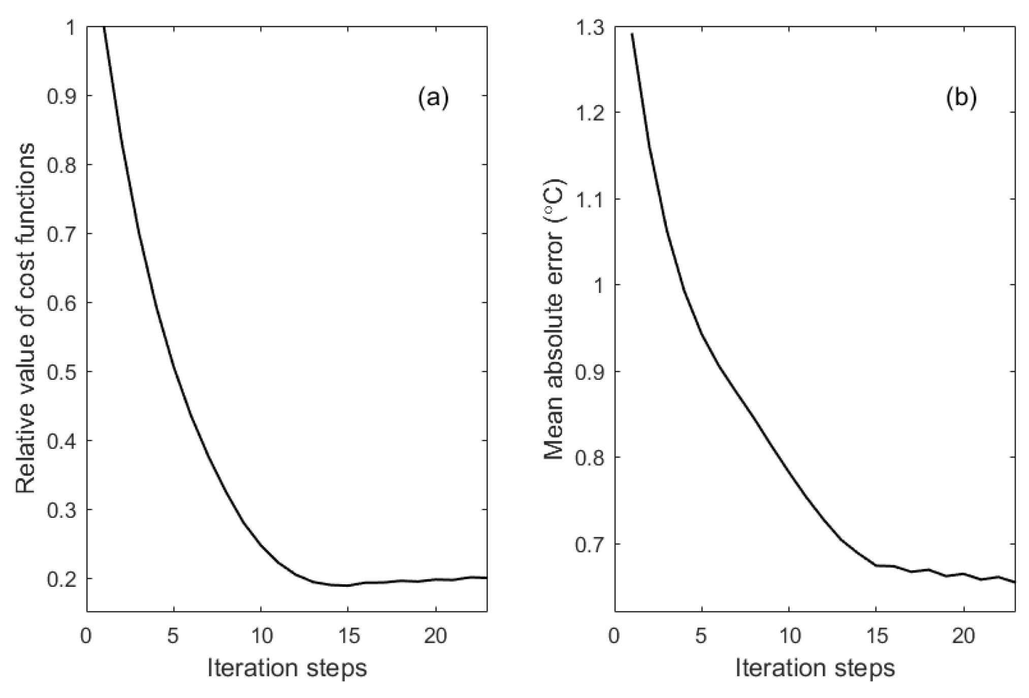
Repeat steps (2) to (6) until the error reduces to a steady state or reaches the preset maximum number of inversion steps, and the inversion ends.

4. Numerical Experiments

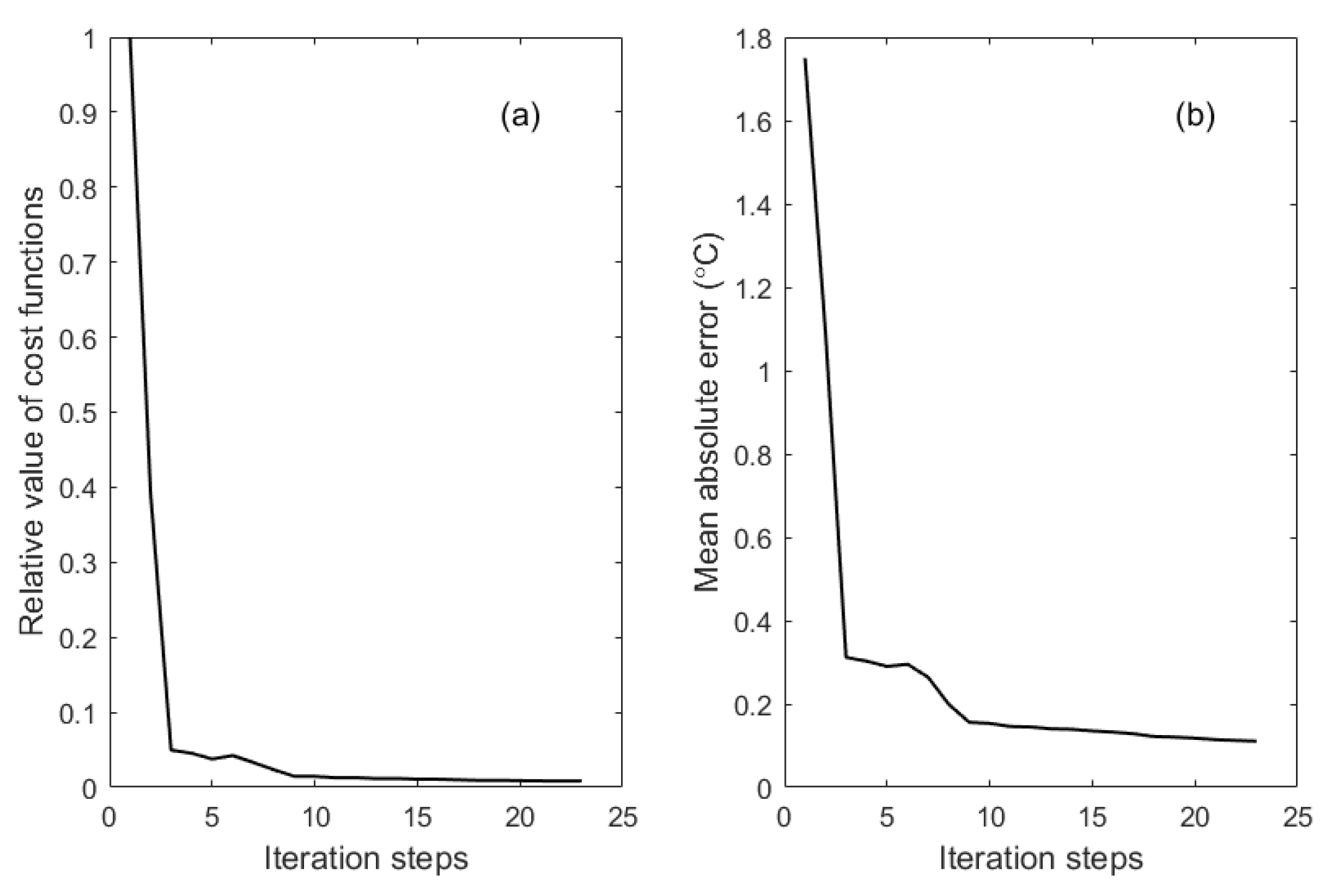
4.1. Ideal Experiment

In this section, we describe the two ideal experiments which were performed to invert two different given initial temperature fields. Feasibility and validity of the adjoint assimilation model were verified by analyzing the temperature of the inversion and the given temperature field.

The initial field I was constructed according to the spatial distribution characteristics of the annual mean temperature which decreases from southeast to northwest of the South China Sea. In addition, the annual mean temperature field was directly used to construct the initial field II (Figure 2).

The two given initial temperature fields were put into the forward model to generate “observations”. The selection method was to take SST at 0:00 a.m. every day except the initial moment as the “surface observations”, and 50 groups of “vertical observations” were selected at different time near the Argo observation in the practical experiment (Figure 3). The corresponding “observations” wwere assimilated respectively, and a distribution of SST temperature decrease from south to north was given as the estimated temperature background distribution (Figure 4). Inversion of the initial field I and II were carried out according to the steps described in Section 3.3.

In the two ideal experiments, the mean absolute error (MAE) between the simulations and the “observations” was reduced from 1.74 °C and 1.87 °C without data assimilation to 0.13 °C and 0.14 °C, respectively, by applying the adjoint assimilation model. Due to the large number of observation data and high resolution of SST, spatial distribution characteristics could be observed more obviously. The initial SST obtained by inversion is shown in Figure 5. The MAE and root mean square error (RMSE) between the inverted SST and the given initial temperature field SST were also calculated (

Table 1. Quantitative metrics of ideal experiment results.

Experiment	MAE (°C)		RMSE (°C)
	Initial	Final	Initial	Final
I	1.83	0.19	2.20	0.22
II	1.94	0.24	2.33	0.37

). To depict the error decline process more clearly, the relative value of cost functions was used to describe the change of cost function is shown in Figure 6a and Figure 7a, which can be expressed as: $J\left(i\right)/J\left(1\right)$ (i is the iteration step), and the MAE change related to the iteration steps are represented in Figure 6b and Figure 7b.

Comparing Figure 3 and Figure 5, it can be seen that the SST obtained by the inversion well reflects the spatial distribution characteristics of the given initial SST. Figure 5a shows that the temperature decreases significantly from southeast to northwest, and Figure 5b also shows a similar phenomenon.

The MAE of the temperature field obtained with assimilation and generated “observed data” are 0.13 °C and 0.14 °C, respectively. The MAE between the SST of the inversion field and the given field are 0.19 °C and 0.24 °C respectively, and the RMSE are 0.22 °C and 0.37 °C respectively; all below 16% that before data assimilation. In addition, the spatial distributions of SST errors of two ideal experiments are analyzed to study the possible causes of errors (Figure 8).

As can be seen in Figure 8, the areas with large errors mainly occur near the northeast land boundary and the south boundary. This may require us to minimize the research area near the boundary when using this method. The error spatial distribution is approximately in a strip pattern, which, combined with Figure 4, is closely related to the estimated temperature background distribution. The error is also lower in the cold current region on the east side of Indo-China Peninsula (yellow box in Figure 8); it can be speculated that the hydrodynamic background fields have a certain influence on the results of numerical calculation. Reasonable selection of background field is also an effective means to reduce errors.

Although the amount of vertical data is relatively small, with discontinuous time and space distribution, it can be found in the red box in Figure 8 that the regional errors with the assimilation of “vertical observations” are significantly reduced compared with the nearby region. In order to make the analysis more intuitive, comparison of vertical inversion and observation are present in Figure 9. It can be found that the inversion results of vertical data correspond well with the observations, since the addition of vertical data assimilation can indeed optimize the numerical simulation results.

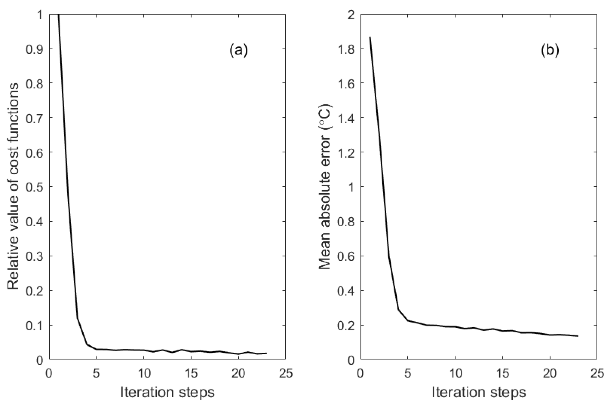
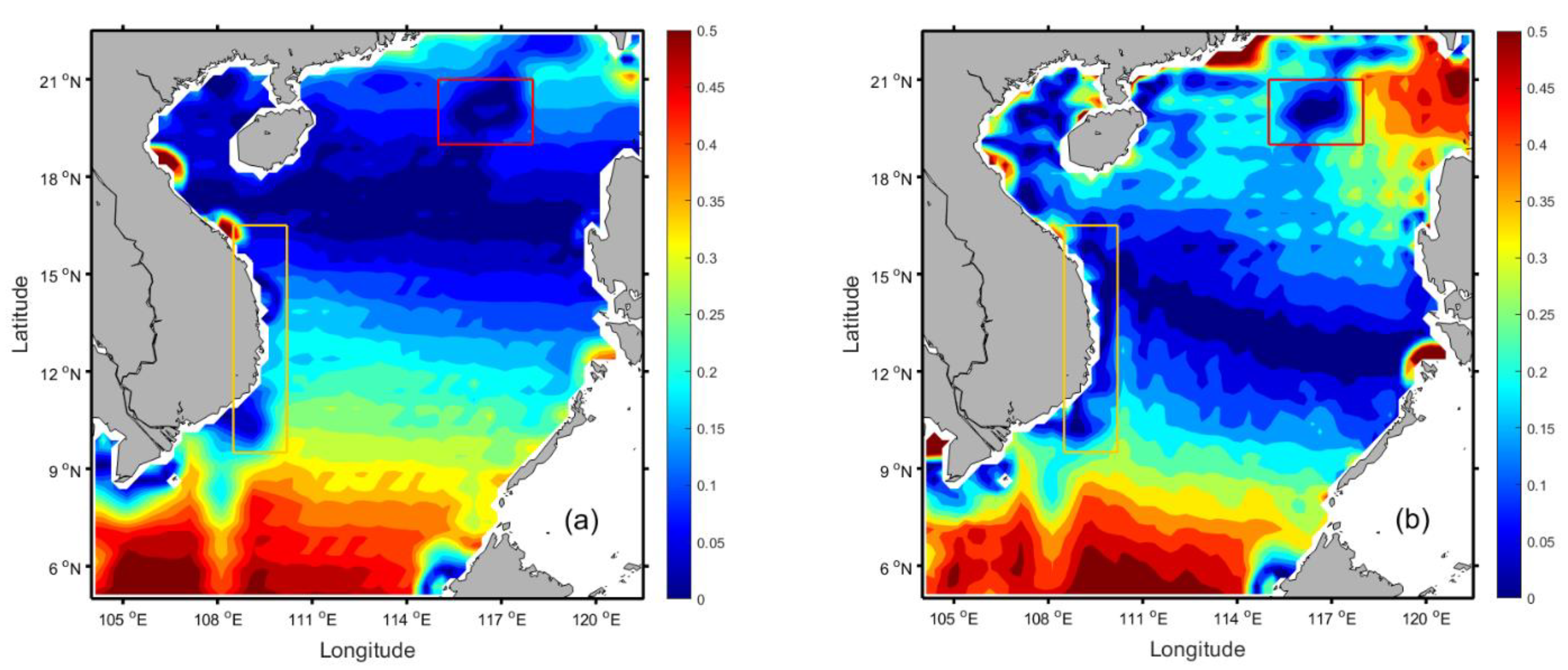
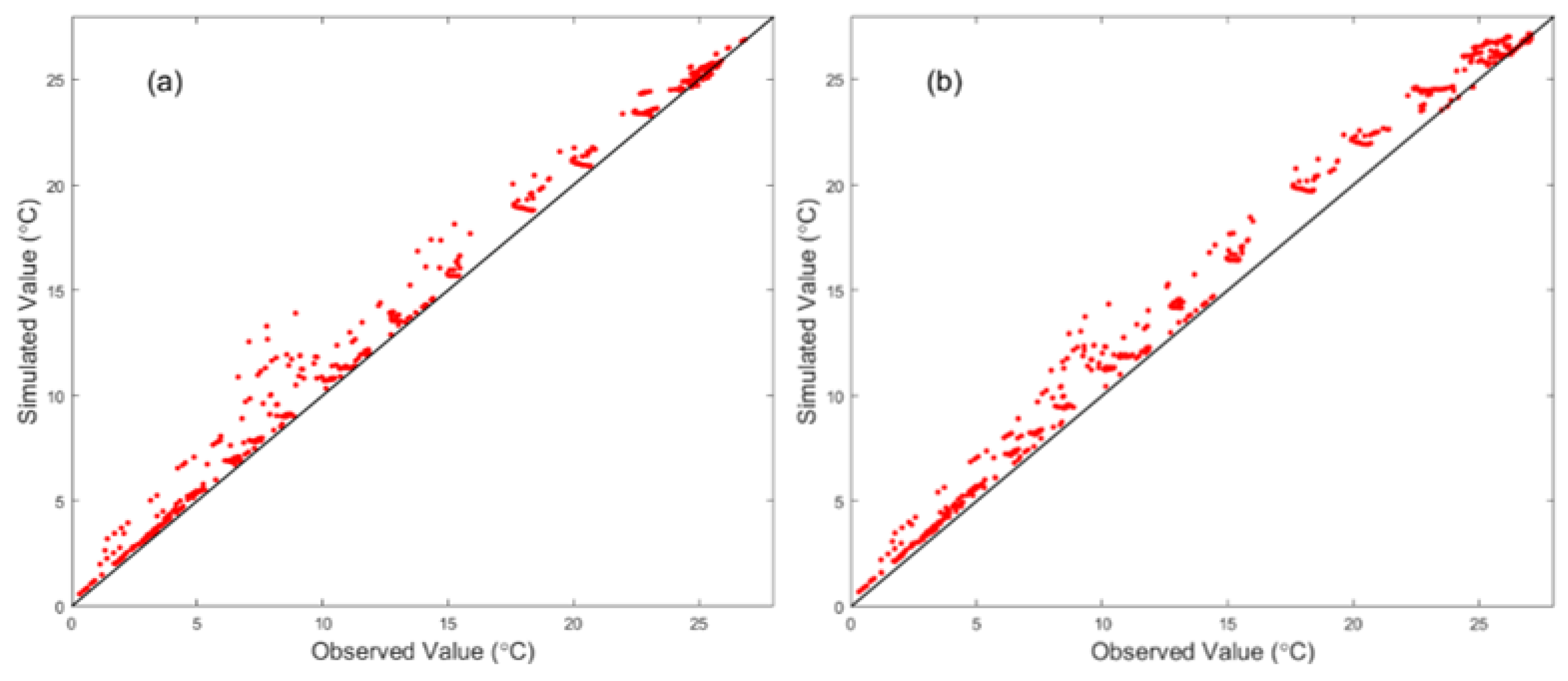
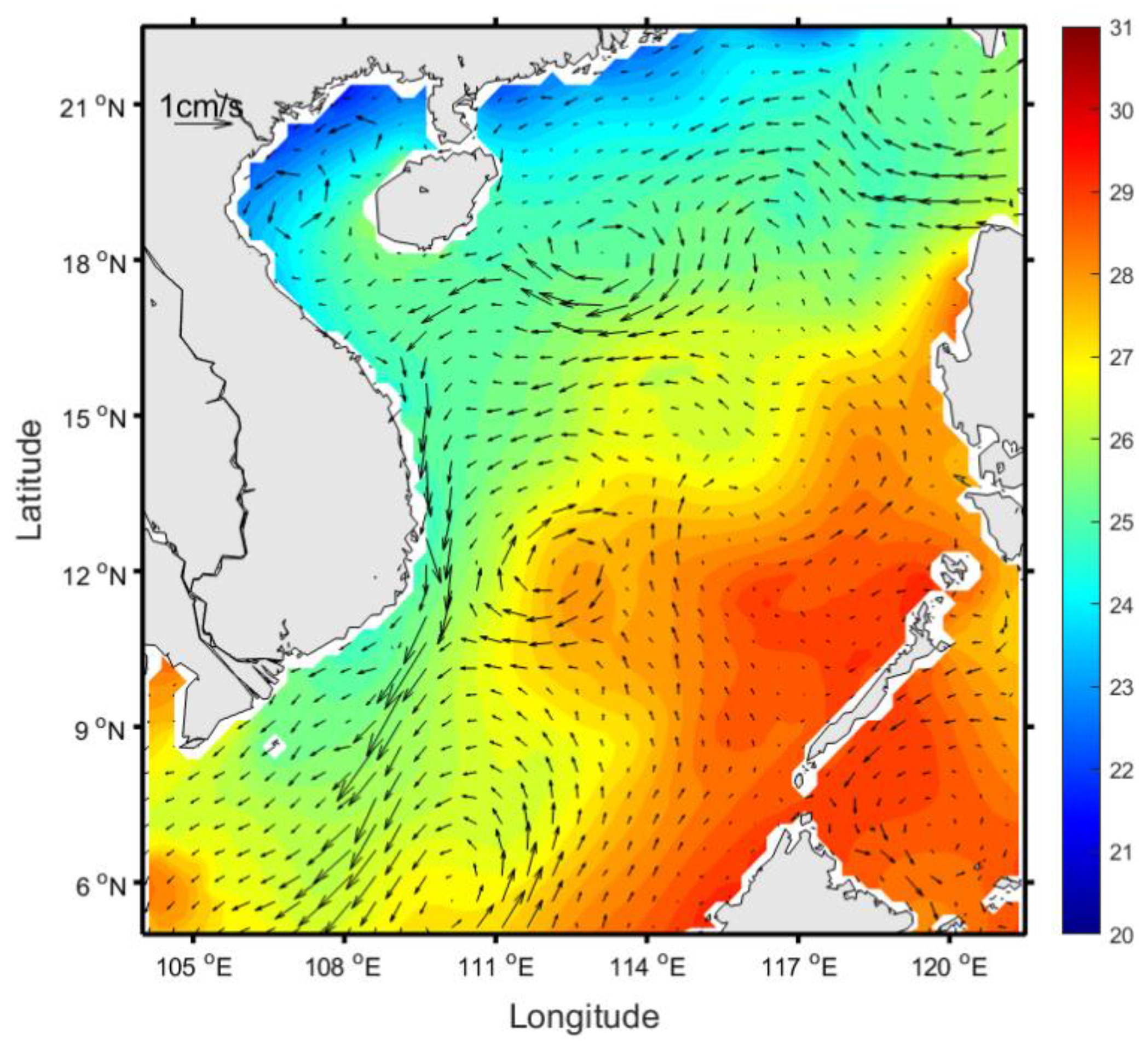
4.2. Practical Experiment

As a world ocean reanalysis dataset compiled by NOAA, WOA is a database of basic physical oceanography and related applications, which has been widely used in oceanographic research and prediction [45,46], and WOA18 is the latest product. The effective combination of observational data and WOA is of great significance for ocean survey and research [45]. In this section, the selection of WOA 2018 as the temperature background field for practical experiment is described.

In the practical experiment, by assimilating the daily SST of the SCS from 2 December 2014 to 30 December 2014 from the GHRSST satellite remote sensing data and 58 groups of Argo float data in December 2014, the climatology temperature in December provided by WOA 2018 (Figure 10) were selected as background filed and corrected to invert the temperature field in the SCS area on 1 December 2014.

The initial temperature field distribution was obtained by assimilating the observation data (Figure 11), and the MAE between the numerical simulation results and the observed data was reduced from 1.29 °C to 0.65 °C. Relative value of cost functions and MAE change related to the iteration steps are also shown in Figure 12.

Combined with previous studies on SST in the SCS [11,47,48], the SST inverted by the adjoint assimilation (Figure 11) was consistent better with the winter distribution in this region than that in Figure 10. By analyzing the inversion of SST, it could be found that the temperature increases generally in the south of 18° N, and the cold current along the Indo-China Peninsula was more obvious. The temperature rise made the isothermal line show northeast-southwest trend, and there was a slightly protruding shape in the middle, which is consistent with the flow field distribution.

5. Conclusions and Discussion

SWT is closely related to climate change, and it is an important parameter in driving the global water cycle. At the same time, it affects the development and utilization of fishery resources through the marine ecological functions, which is of great significance to the research and prediction of sea water temperature. The accuracy of SWT numerical simulation and prediction is heavily dependent on the quality of initial values. Although various ocean models are gradually improving, the initial field is still difficult to determine. In this paper, the SCS is taken as the research area. Based on the temperature transport adjoint assimilation model, the initial temperature field is inverted by assimilating the surface temperature and vertical temperature observations.

The two given initial temperature fields were successfully inverted in the ideal experiments. The inversion SST distributions were very close to the given distributions with low MAE and RMSE. Furthermore, in the area with vertical observation data, the error was also reduced, indicating that the inversion method is feasible and valid.

In the practical experiment, the monthly average temperature field of WOA18 was adjusted by assimilating Argo data and GHRSST data, to invert temperature field of the SCS on 1 December 2014. The inversion results show a good agreement with the observations. Compared with other studies on SST in the SCS, the inverted distribution is consistent better with the actual SST distribution than the WOA18. By assimilation, the error between the simulated and observed data is reduced from 1.29 °C to 0.65 °C. In addition, according to the error statistics of vertical observation data, it was also found that the effect of numerical simulation is ideal.

The results of ideal and practical experiments show that the error between the numerical simulation and the observation is highly reduced by the use of observed data, to a great extent with the assimilation method. It indicates that adjoint assimilation can provide a 3D initial field that better reflects the actual distribution for the numerical simulation of temperature. However, the error distribution shows that the method depends on the quality and quantity of data to a certain extent, and sufficient data can be better combined with the model.

References

1. Kawai, Y.; Wada, A. Diurnal sea surface temperature variation and its impact on the atmosphere and ocean: A review. J. Oceanogr. 2007, 63, 721–744. [Google Scholar] [CrossRef]
2. Wu, Z.; Huang, N.E.; Wallace, J.M.; Smoliak, B.V.; Chen, X. On the time-varying trend in global mean surface temperature. Clim. Dyn. 2011, 37, 759–773. [Google Scholar] [CrossRef] [Green Version]
3. Lau, N.C. Interactions between Global SST Anomalies and the Midlatitude Atmospheric Circulation. Bull. Am. Meteorol. Soc. 1997, 78, 21–33. [Google Scholar] [CrossRef] [Green Version]
4. Zhu, X.; Liu, Z. Tropical SST response to global warming in the twentieth century. J. Clim. 2009, 22, 1305–1312. [Google Scholar] [CrossRef] [Green Version]
5. Seager, R.; Zebiak, S.E.; Cane, M.A. A model of the tropical Pacific Sea surface temperature climatology. J. Geophys. Res. 1988, 93, 1265–1280. [Google Scholar] [CrossRef]
6. Su, J.; Wang, H.; Yang, H.; Drange, H.; Gao, Y.; Bentsen, M. Role of the atmospheric and oceanic circulation in the tropical pacific SST changes. J. Clim. 2008, 21, 2019–2034. [Google Scholar] [CrossRef]
7. Roxy, M.; Tanimoto, Y. Influence of sea surface temperature on the intraseasonal variability of the South China Sea summer monsoon. Clim. Dyn. 2012, 39, 1209–1218. [Google Scholar] [CrossRef] [Green Version]
8. Sugimoto, S. Influence of SST anomalies on winter turbulent heat fluxes in the eastern Kuroshio-Oyashio confluence region. J. Clim. 2014, 27, 9349–9358. [Google Scholar] [CrossRef]
9. Zhang, L.; Wu, L.; Lin, X.; Wu, D. Modes and mechanisms of sea surface temperature low-frequency variations over the coastal China seas. J. Geophys. Res. Ocean. 2010, 115, 1–13. [Google Scholar] [CrossRef]
10. Yuan, J.; Wang, D.; Liu, C.; Wen, G. Validation of Microwave-Infrared, Tropical Rainfall Measuring Mission Microwave Im ager and Advanced Microwave Scanning Radiometer—Earth observing system and WindSat-derived sea surface temperatures in coastal waters of the northern South China Sea. Aquat. Ecosyst. Heal. Manag. 2016, 19, 260–269. [Google Scholar] [CrossRef]
11. Ren, S.; Zhu, X.U.; Drevillon, A.; Wang, H.; Zhang, Y.; Zu, Z.; Li, A. Detection of SST fronts from a high-resolution model and its preliminary results in the south China sea. J. Atmos. Ocean. Technol. 2021, 38, 387–403. [Google Scholar] [CrossRef]
12. Kawai, Y.; Kawamura, H.; Takahashi, S.; Hosoda, K.; Murakami, H.; Kachi, M.; Guan, L. Satellite-based high-resolution global optimum interpolation sea surface temperature data. J. Geophys. Res. Ocean. 2006, 111, 1–17. [Google Scholar] [CrossRef] [Green Version]
13. Zhang, R.H.; Busalacchi, A.J.; Murtugudde, R.G. Improving SST anomaly simulations in a layer ocean model with an embedded entrainment temperature submodel. J. Clim. 2006, 19, 4638–4663. [Google Scholar] [CrossRef]
14. Zhu, J.; Kumar, A.; Wang, H.; Huang, B. Sea surface temperature predictions in NCEP CFSv2 using a simple ocean initialization scheme. Mon. Weather Rev. 2015, 143, 3176–3191. [Google Scholar] [CrossRef]
15. Peng, S.Q.; Xie, L. Effect of determining initial conditions by four-dimensional variational data assimilation on storm surge forecasting. Ocean Model. 2006, 14, 1–18. [Google Scholar] [CrossRef] [Green Version]
16. Liu, X.; Wang, Q.; Mu, M. Optimal Initial Error Growth in the Prediction of the Kuroshio Large Meander Based on a High-resolution Regional Ocean Model. Adv. Atmos. Sci. 2018, 35, 1362–1372. [Google Scholar] [CrossRef]
17. Kolmogoroff, A.N. The local structure of turbulence in incompressible viscous fluid for very large Reynolds numbers. C. R. Acad. Sci. URSS 1941, 30, 301–305. [Google Scholar]
18. Wang, S.; Su, Y. A model for prediction SST in linited region-II. The model’s physical equation. Acta Oceanol. Sin. 1992, 11, 57–66. [Google Scholar]
19. Zhang, W.G.; Wilkin, J.L.; Arango, H.G. Towards an integrated observation and modeling system in the New York Bight using variational methods. Part I: 4DVAR data assimilation. Ocean Model. 2010, 35, 119–133. [Google Scholar] [CrossRef] [Green Version]
20. Song, Z.; Qiao, F.; Yang, Y.; Yuan, Y. An improvement of the too cold tongue in the tropical Pacific with the development of an ocean-wave-atmosphere coupled numerical model. Prog. Nat. Sci. 2007, 17, 576–583. [Google Scholar]
21. Xu, Z.; Li, M.; Patricola, C.M.; Chang, P. Oceanic origin of southeast tropical Atlantic biases. Clim. Dyn. 2014, 43, 2915–2930. [Google Scholar] [CrossRef]
22. Ohlmann, J.C.; Siegel, D.A. Ocean radiant heating. Part II: Parameterizing solar radiation transmission through the upper ocean. J. Phys. Oceanogr. 2000, 30, 1849–1865. [Google Scholar] [CrossRef] [Green Version]
23. Riser, S.C.; Freeland, H.J.; Roemmich, D.; Wijffels, S.; Troisi, A.; Belbéoch, M.; Gilbert, D.; Xu, J.; Pouliquen, S.; Thresher, A.; et al. Fifteen years of ocean observations with the global Argo array. Nat. Clim. Chang. 2016, 6, 145–153. [Google Scholar] [CrossRef] [Green Version]
24. Hosoda, S.; Ohira, T.; Nakamura, T. A Monthly mean dataset of global oceanic temperature and salinity derived from Argo float observations. JAMSTEC Rep. Res. Dev. 2008, 8, 47–59. [Google Scholar] [CrossRef] [Green Version]
25. Zhou, C.; Ding, X.; Zhang, J.; Yang, J.; Ma, Q. An objective algorithm for reconstructing the three-dimensional ocean temperature field based on Argo profiles and SST data. Ocean Dyn. 2017, 67, 1523–1533. [Google Scholar] [CrossRef]
26. Sasaki, Y. Some Basic Formalisms in Numerical Variational Analysis. Mon. Weather Rev. 1970, 98, 875–883. [Google Scholar] [CrossRef] [Green Version]
27. Andreu-Burillo, I.; Holt, J.; Proctor, R.; Annan, J.D.; James, I.D.; Prandle, D. Assimilation of sea surface temperature in the POL Coastal Ocean Modelling System. J. Mar. Syst. 2007, 65, 27–40. [Google Scholar] [CrossRef]
28. Peng, S.Q.; Xie, L.; Pietrafesa, L.J. Correcting the errors in the initial conditions and wind stress in storm surge simulation using an adjoint optimal technique. Ocean Model. 2007, 18, 175–193. [Google Scholar] [CrossRef]
29. Zhu, X.; Zu, Z.; Ren, S.; Zhang, Y.; Zhang, M.; Wang, H. The improvements to the regional South China Sea Operational Oceanography Forecasting System. Ocean Sci. Discuss. 2020, 1–37. [Google Scholar] [CrossRef]
30. Chen, D.; Busalacchi, A.J.; Rothstein, L.M. The roles of vertical mixing, solar radiation, and wind stress in a model simulation of the sea surface temperature seasonal cycle in the tropical Pacific Ocean. J. Geophys. Res. 1994, 99, 20345–20359. [Google Scholar] [CrossRef]
31. Murtugudde, R.; Busalacchi, A.J. Interannual variability of the dynamics and thermodynamics of the tropical Indian Ocean. J. Clim. 1999, 12, 2300–2326. [Google Scholar] [CrossRef]
32. Fan, W.; Lv, X. Data assimilation in a simple marine ecosystem model based on spatial biological parameterizations. Ecol. Modell. 2009, 220, 1997–2008. [Google Scholar] [CrossRef]
33. Zhang, J.; Lu, X.; Wang, P.; Wang, Y.P. Study on linear and nonlinear bottom friction parameterizations for regional tidal models using data assimilation. Cont. Shelf Res. 2011, 31, 555–573. [Google Scholar] [CrossRef]
34. Wang, C.; Li, X.; Lv, X. Numerical study on initial field of pollution in the Bohai Sea with an adjoint method. Math. Probl. Eng. 2013, 2013. [Google Scholar] [CrossRef] [Green Version]
35. Wang, D.; Cao, A.; Zhang, J.; Fan, D.; Liu, Y.; Zhang, Y. A three-dimensional cohesive sediment transport model with data assimilation: Model development, sensitivity analysis and parameter estimation. Estuar. Coast. Shelf Sci. 2018, 206, 87–100. [Google Scholar] [CrossRef]
36. Liu, Y.; Yu, J.; Shen, Y.; Lv, X. A modified interpolation method for surface total nitrogen in the Bohai Sea. J. Atmos. Ocean. Technol. 2016, 33, 1509–1517. [Google Scholar] [CrossRef]
37. Zong, X.; Xu, M.; Xu, J.; Lv, X. Improvement of the ocean pollutant transport model by using the surface spline interpolation. Tellus, Ser. A Dyn. Meteorol. Oceanogr. 2018, 70, 1–13. [Google Scholar] [CrossRef] [Green Version]
38. Zheng, Q.; Li, X.; Lv, X. Application of dynamically constrained interpolation methodology to the surface nitrogen concentration in the bohai sea. Int. J. Environ. Res. Public Health 2019, 16, 2400. [Google Scholar] [CrossRef] [Green Version]
39. Li, X.; Zheng, Q.; Lv, X. Application of the spline interpolation in simulating the distribution of phytoplankton in a marine npzd type ecosystem model. Int. J. Environ. Res. Public Health 2019, 16, 2664. [Google Scholar] [CrossRef] [Green Version]
40. Wang, C.; Lan, J.; Wang, G. Climatology and seasonal variability of theMindanao Undercurrent based on OFES data. Acta Oceanol. Sin. 2013, 32, 14–20. [Google Scholar] [CrossRef]
41. Tomita, H.; Hihara, T.; Kako, S.; Kubota, M.; Kutsuwada, K. An introduction to J-OFURO3, a third-generation Japanese ocean flux data set using remote-sensing observations. J. Oceanogr. 2019, 75, 171–194. [Google Scholar] [CrossRef] [Green Version]
42. Locarnini, R.; Mishonov, A.; Baranova, O.; Boyer, T.; Zweng, M.; Garcia, H.; Reagan, J.; Seidov, D.; Weathers, K.; Paver, C.; et al. World Ocean Atlas 2018, Volume 1: Temperature; U.S. Department of Commerce: Washington, DC, USA, 2019.
43. Ullman, D.; Wilson, R. Model parameter estimation from data assimilation modeling: Temporal and spatial variability of the bottom drag coefficient. J. Geophys. Res. 1998, 103, 5531–5549. [Google Scholar] [CrossRef]
44. Lu, X.; Zhang, J. Numerical study on spatially varying bottom friction coefficient of a 2D tidal model with adjoint method. Cont. Shelf Res. 2006, 26, 1905–1923. [Google Scholar] [CrossRef]
45. Levitus, S.; Antonov, J.I.; Boyer, T.P.; Locarnini, R.A.; Garcia, H.E.; Mishonov, A.V. Global ocean heat content 1955–2008 in light of recently revealed instrumentation problems. Geophys. Res. Lett. 2009, 36, 1–6. [Google Scholar] [CrossRef]
46. Huang, C.; Wu, M.; Huang, X.; Cao, J.; He, J.; Chen, C.; Zhai, G.; Deng, K.; Lu, X. Reconstruction and evaluation of the full-depth sound speed profile with world ocean atlas 2018 for the hydrographic surveying in the deep sea waters. Appl. Ocean Res. 2020, 101, 102201. [Google Scholar] [CrossRef]
47. Shu, Y.; Zhu, J.; Wang, D.; Yan, C.; Xiao, X. Performance of four sea surface temperature assimilation schemes in the South China Sea. Cont. Shelf Res. 2009, 29, 1489–1501. [Google Scholar] [CrossRef]
48. Yu, Y.; Zhang, H.R.; Jin, J.; Wang, Y. Trends of sea surface temperature and sea surface temperature fronts in the South China Sea during 2003–2017. Acta Oceanol. Sin. 2019, 38, 106–115. [Google Scholar] [CrossRef]
Figure 1. Monthly mean surface flow field in December (unit: cm/s).
Jmse 09 00760 g001
Figure 2. Given SST distribution I (a) and II (b) (unit: °C).
Jmse 09 00760 g002
Figure 3. Vertical data position (the black dots denote Argo observation points, the red asterisks denote selected points in ideal experiment).
Jmse 09 00760 g003
Figure 4. The estimated background SST distribution (unit: °C).
Jmse 09 00760 g004
Figure 5. Inverted SST distribution I (a) and II (b) (unit: °C).
Jmse 09 00760 g005
Figure 6. Cost function (a) and MAE (b) change related to the iteration steps in ideal experiment I.
Jmse 09 00760 g006
Figure 7. Cost function (a) and MAE (b) change related to the iteration steps in ideal experiment II.
Jmse 09 00760 g007
Figure 8. The error magnitude space distribution of ideal experiment I (a) and II (b) (unit: °C).
Jmse 09 00760 g008
Figure 9. Comparison of simulated and observed values of vertical data in ideal experiments I (a) and II (b), the red dots denote interpolated observations.
Jmse 09 00760 g009
Figure 10. Distribution of monthly mean SST in December from WOA18 (unit: °C) and surface flow field (unit: cm/s).
Jmse 09 00760 g010
Figure 11. Inverted sea surface temperature distribution (unit: °C) and surface flow field.
Jmse 09 00760 g011
Figure 12. Cost function (a) and MAE (b) change related to the iteration steps.
Jmse 09 00760 g012