
Techno-Economic Assessment of Offshore Wind Energy in the Philippines


Abstract
:1. Introduction
1.1. Statement of the Problem
- Methodologies on techno-economic assessment of offshore wind energy have not been applied to the Philippine setting.
- A notion exists that it is a risky investment with high cost and uncertainty in return.
- There is no readily available and reliable information for investments regarding the viability of offshore wind farms in the Philippines.
- There has been no formulation for the recommendation of the viability of offshore wind energy in the Philippines.
1.2. Objectives of the Study
- To develop a methodology for the techno-economic assessment of offshore wind farms in the Philippines.
- To assess the wind resource in the Philippine oceans for the potential of putting up an offshore wind farm.
- To investigate the economic viability of constructing an offshore wind farm in the Philippines through LCOE.
- To formulate a recommendation for the viability of OWF in the Philippines.
1.3. Research Significance
1.4. Limitations of the Study
2. Review of Related Literature
2.1. Offshore Wind Farms
2.2. Offshore Wind: Current Status
2.2.1. Installed Capacity
2.2.2. Number of Turbines and Project Area
2.2.3. Distance to Shore and Water Depths
2.2.4. Cost
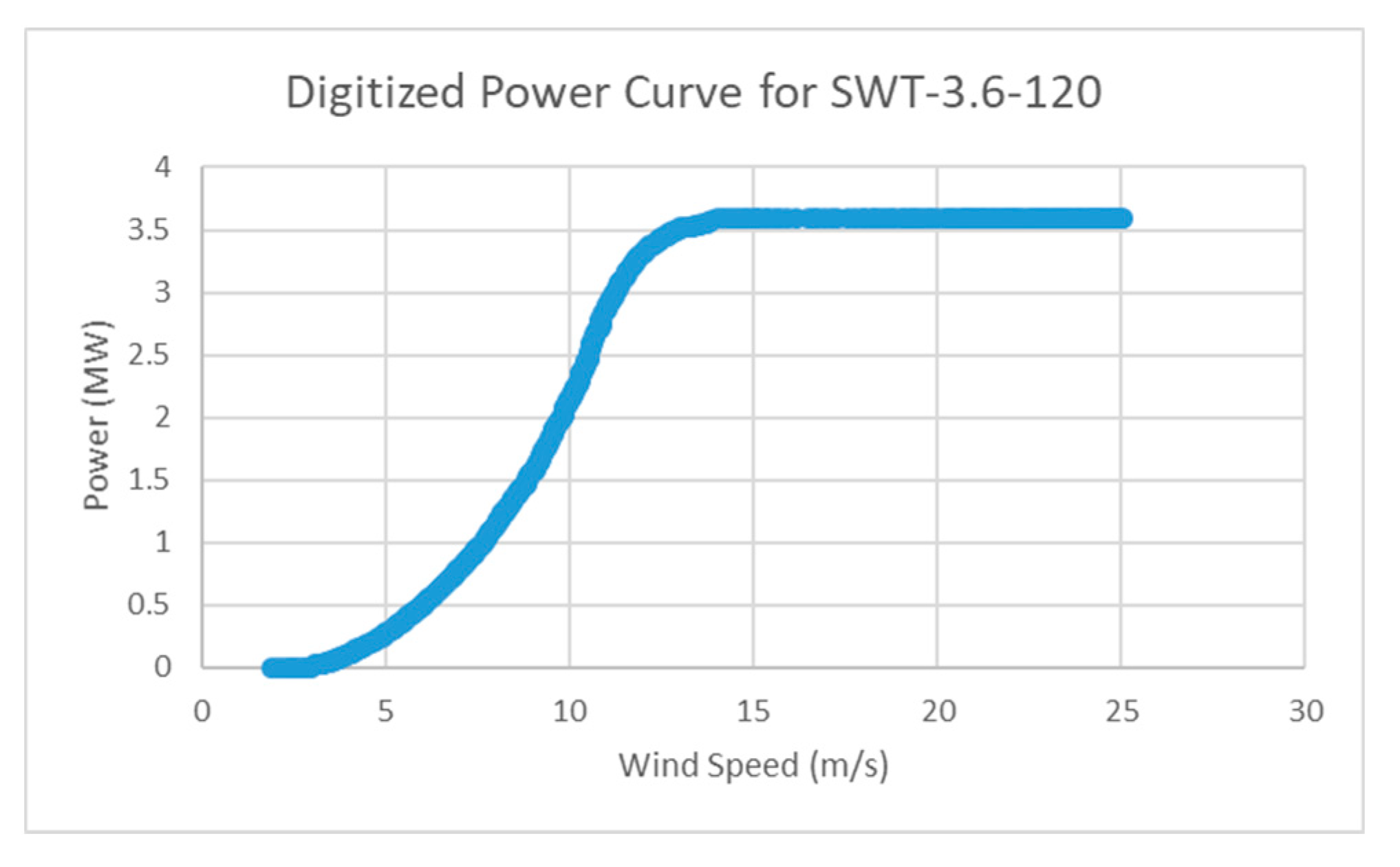
2.2.5. Wind Turbines
2.3. Foundation Technologies
2.4. Renewable Energy Law in the Philippines
2.5. Related Techno-Economic Studies
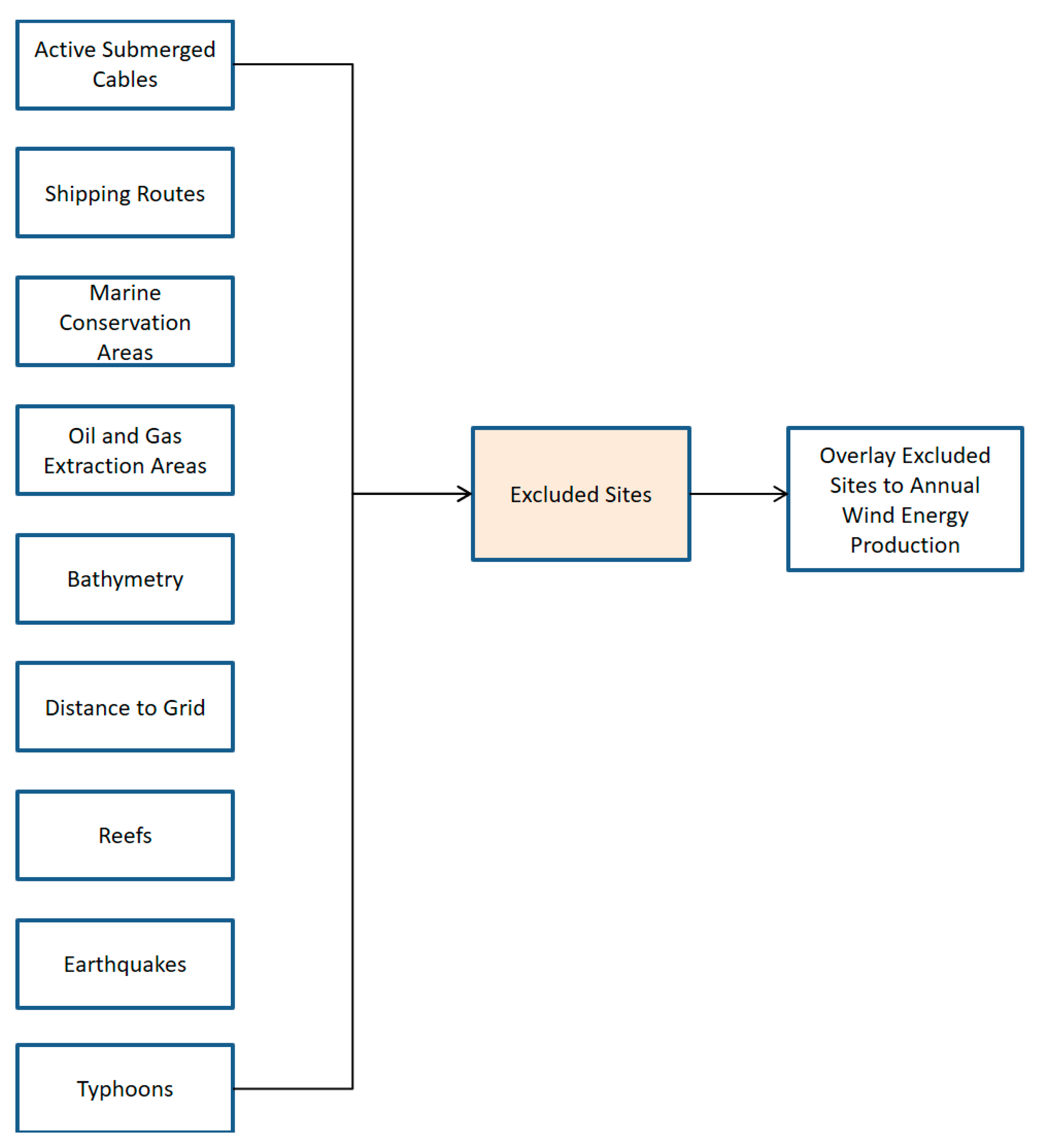
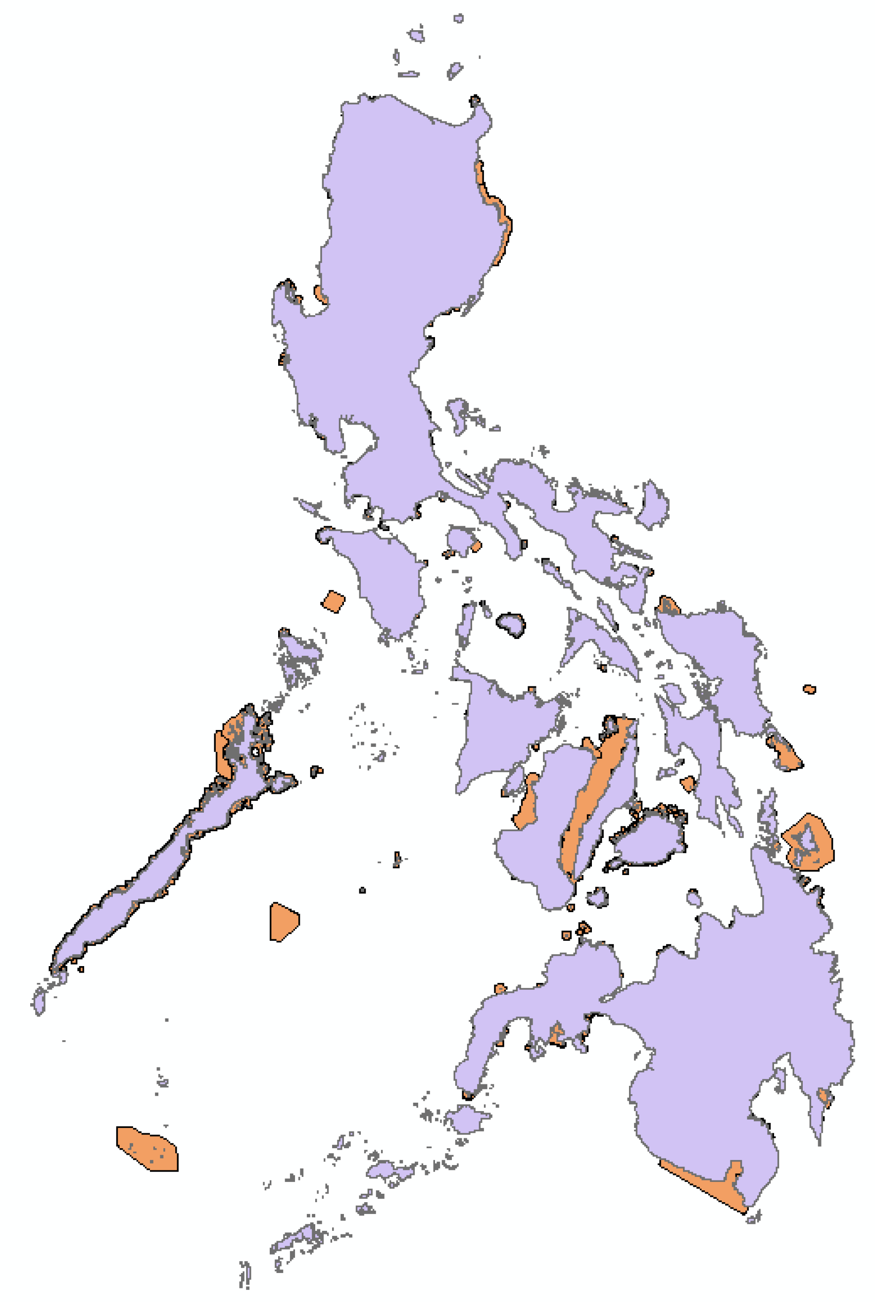
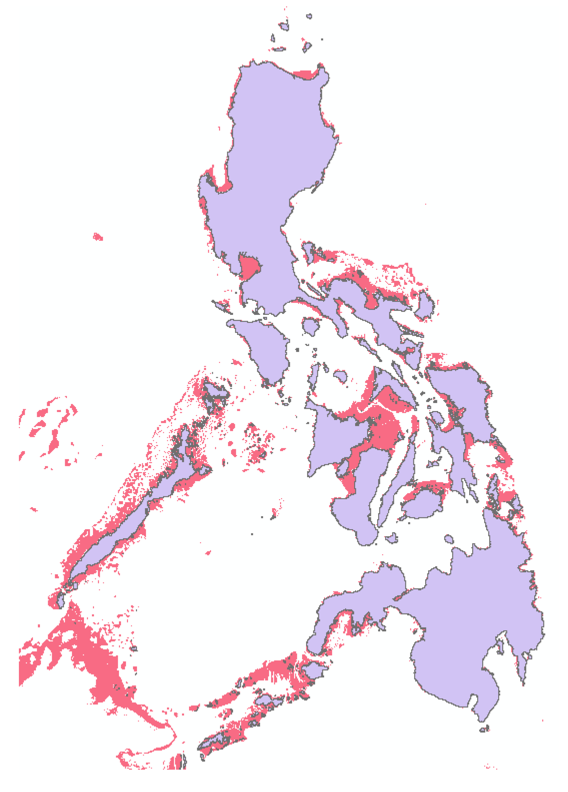
2.6. Exclusion Criteria
2.7. Wind Curtailment
2.8. Data Sources
2.9. Technical Analysis
2.9.1. Power Law
2.9.2. Weibull Model
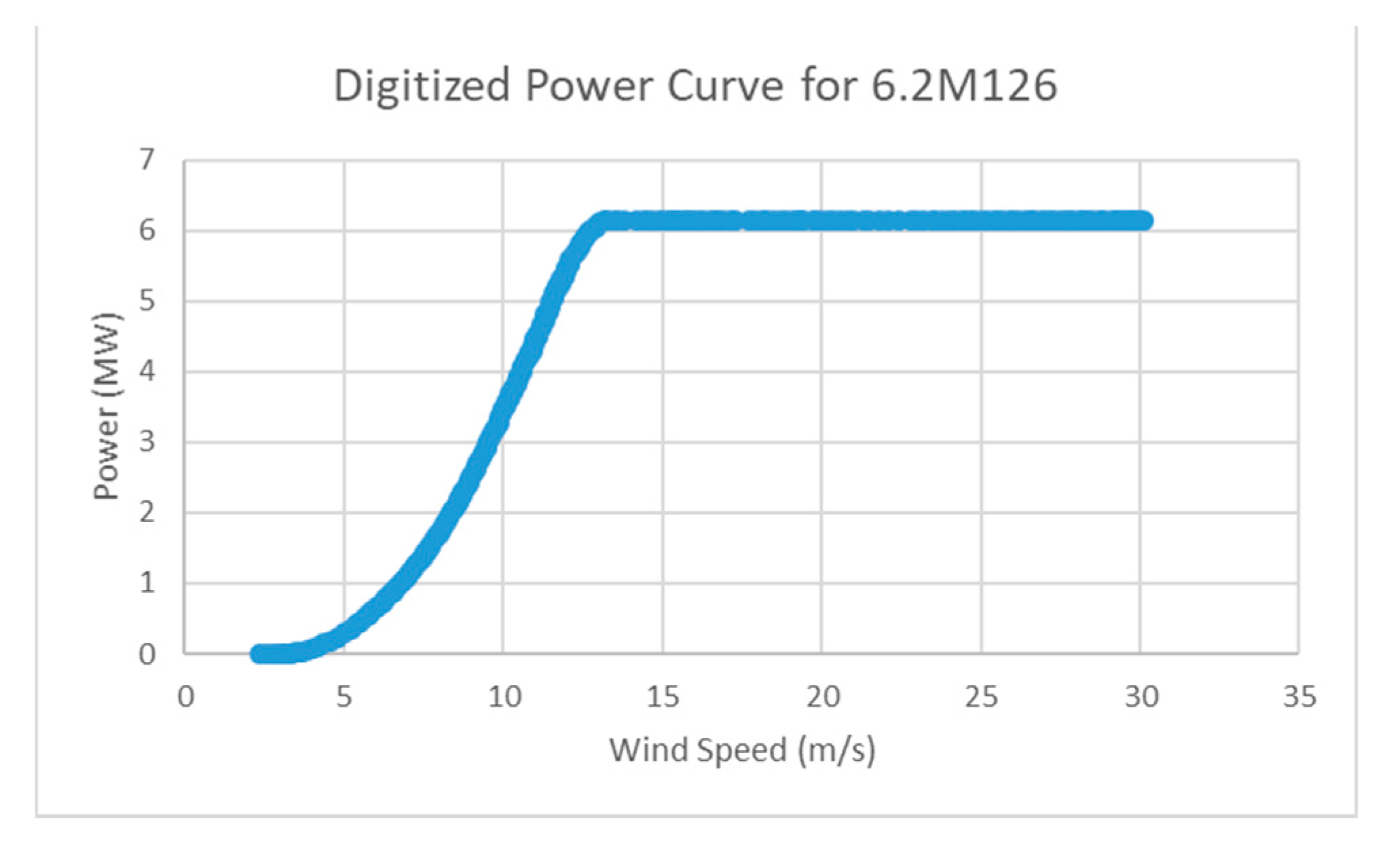
2.9.3. Wind Turbine Power Curve
2.9.4. Wind Power and Wind Power Density
2.9.5. Annual Wind Energy Production
2.9.6. Capacity Factor
2.9.7. Performance
2.9.8. Array Spacing and Number of Turbines
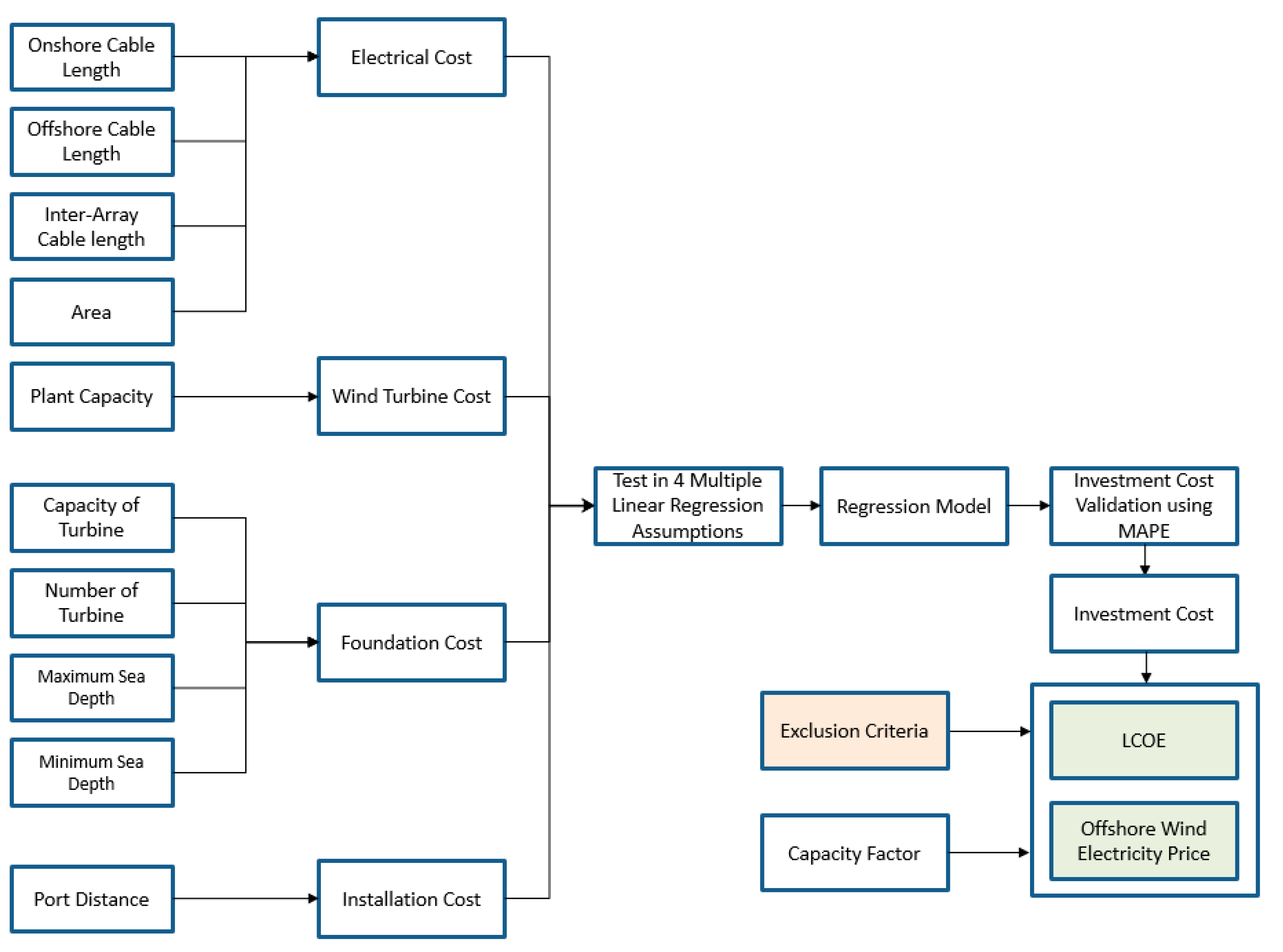
2.10. Economic Analysis
2.10.1. Investment Cost
2.10.2. Multiple Linear Regression
2.10.3. Multiple Regression Assumptions
2.10.4. Net Present Value
2.10.5. Levelized Cost of Electricity
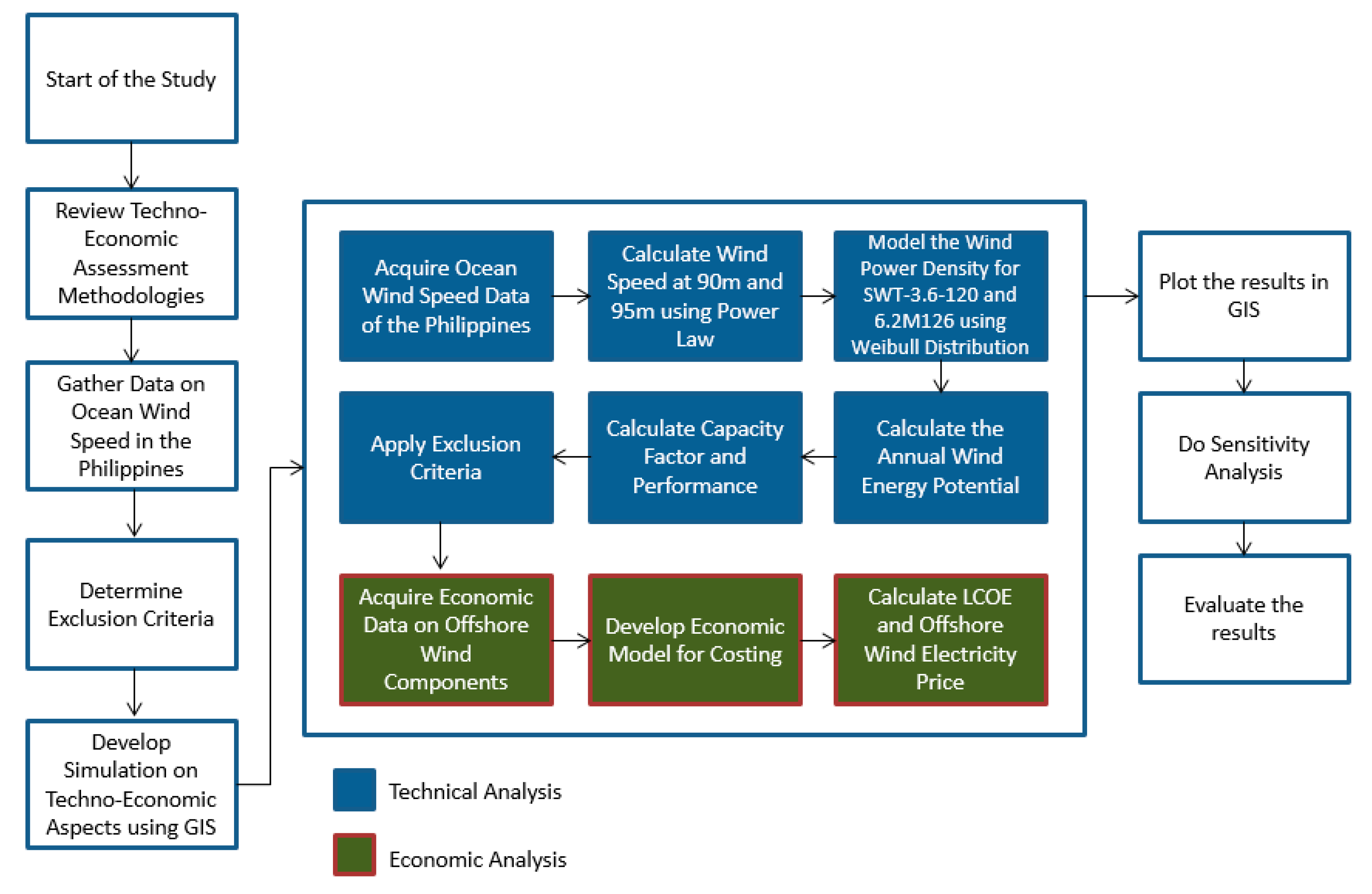
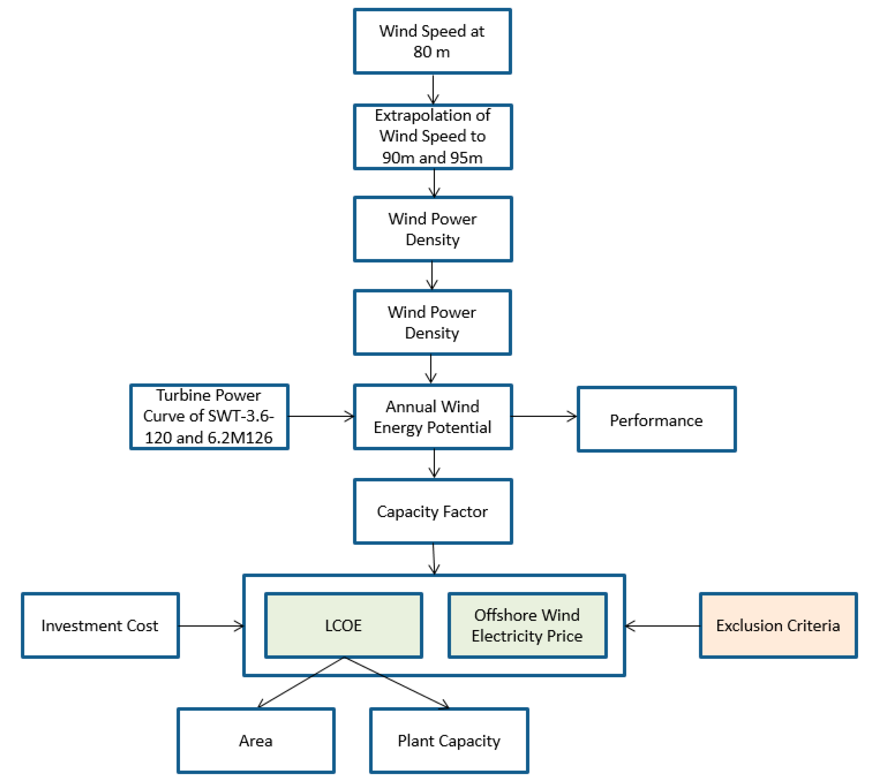
3. Methodology
3.1. Framework of Methodology
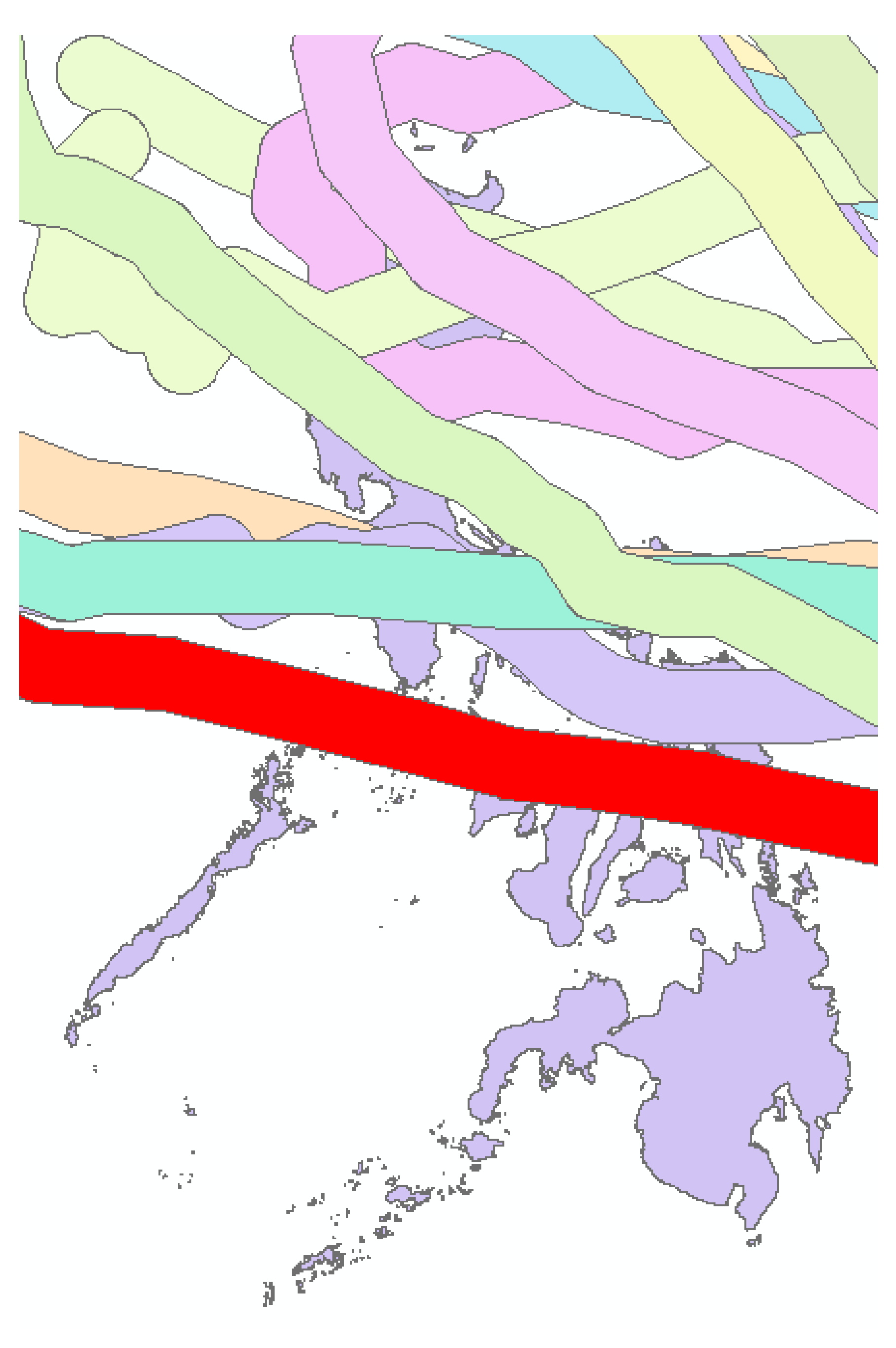
3.1.1. Exclusion Criteria
3.1.2. Technical Analysis
3.1.3. Economic Analysis
3.1.4. Sensitivity Analysis
3.2. R Statistical Software
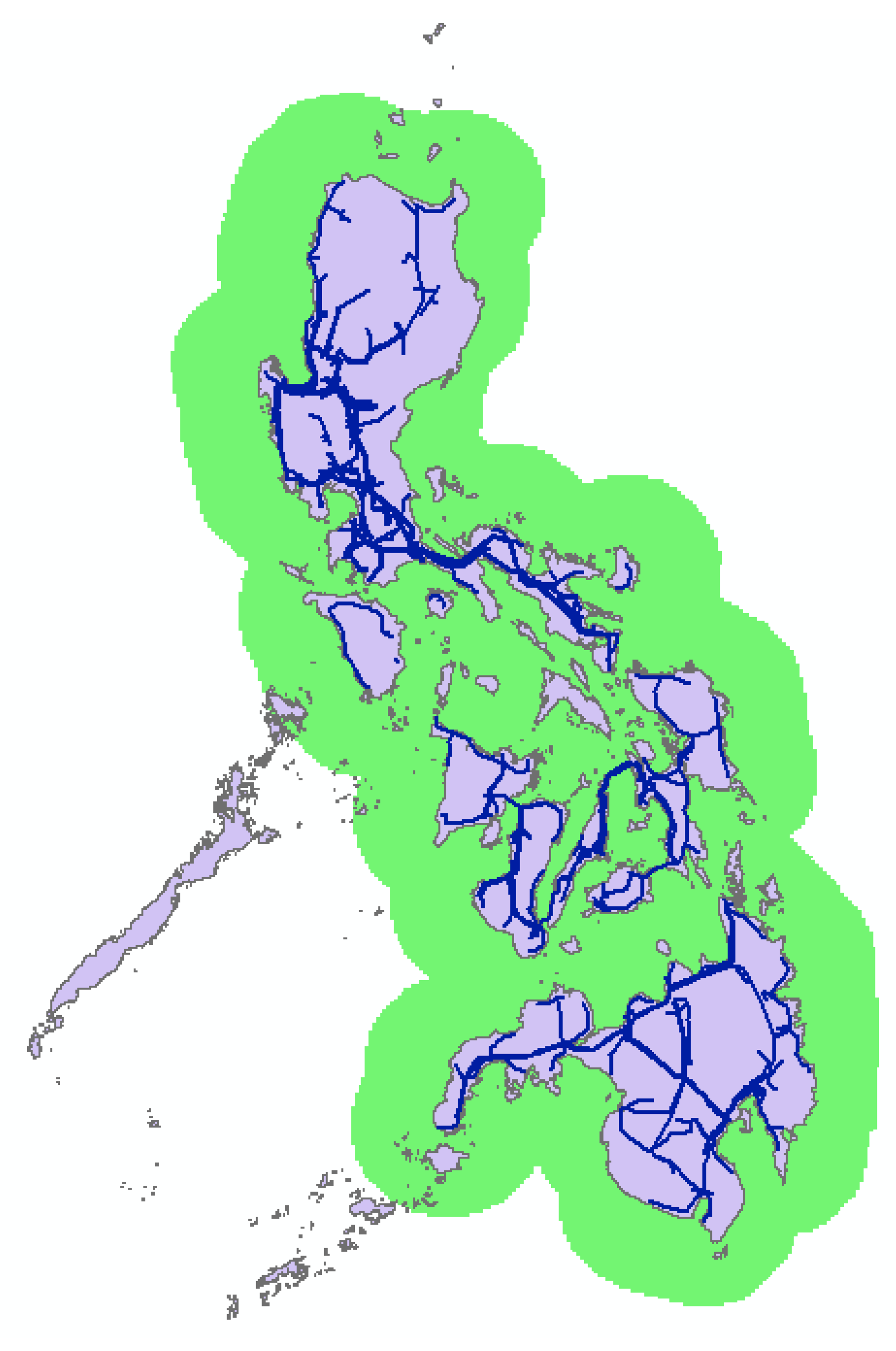
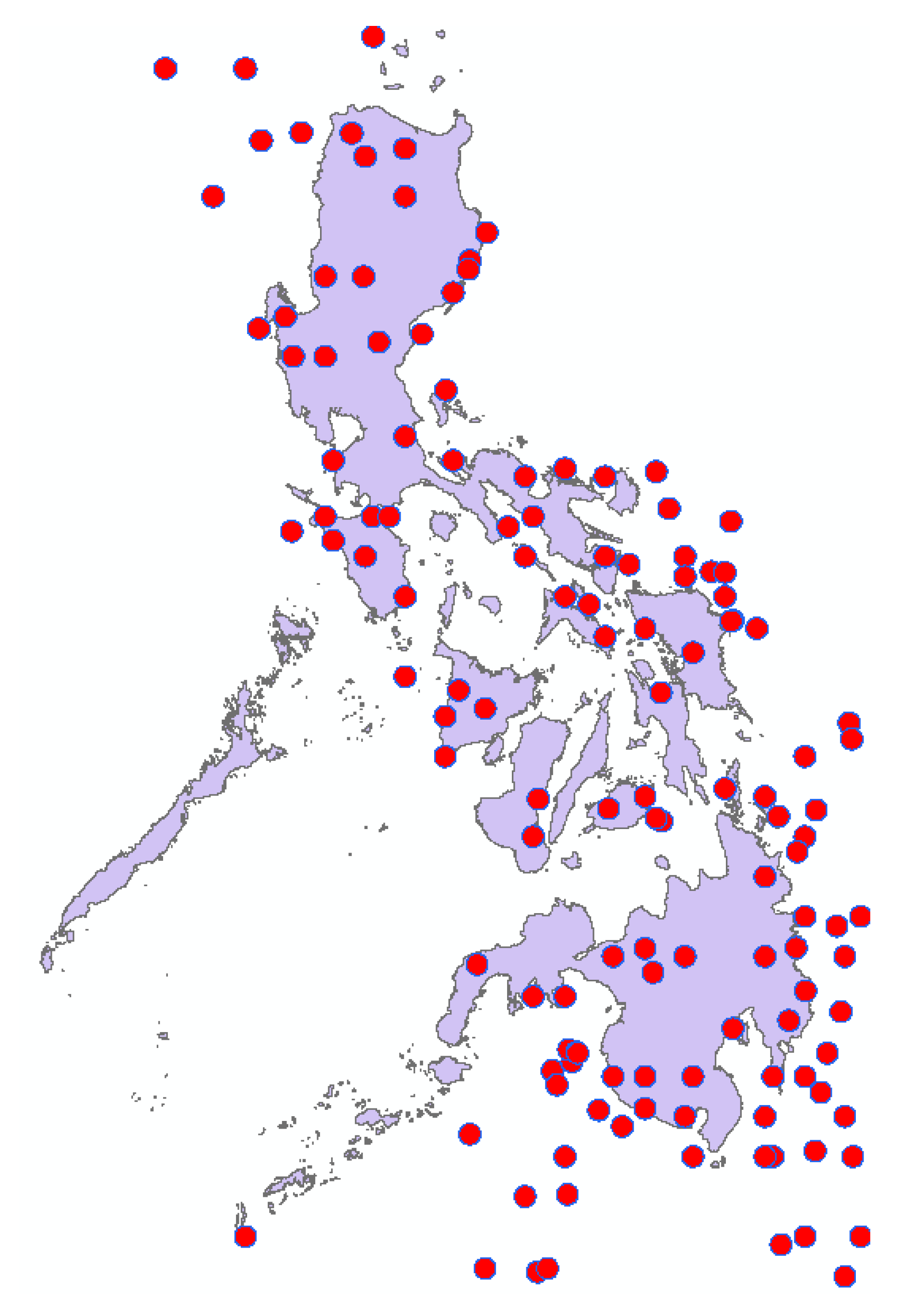
3.3. GIS Software
4. Results and Discussions
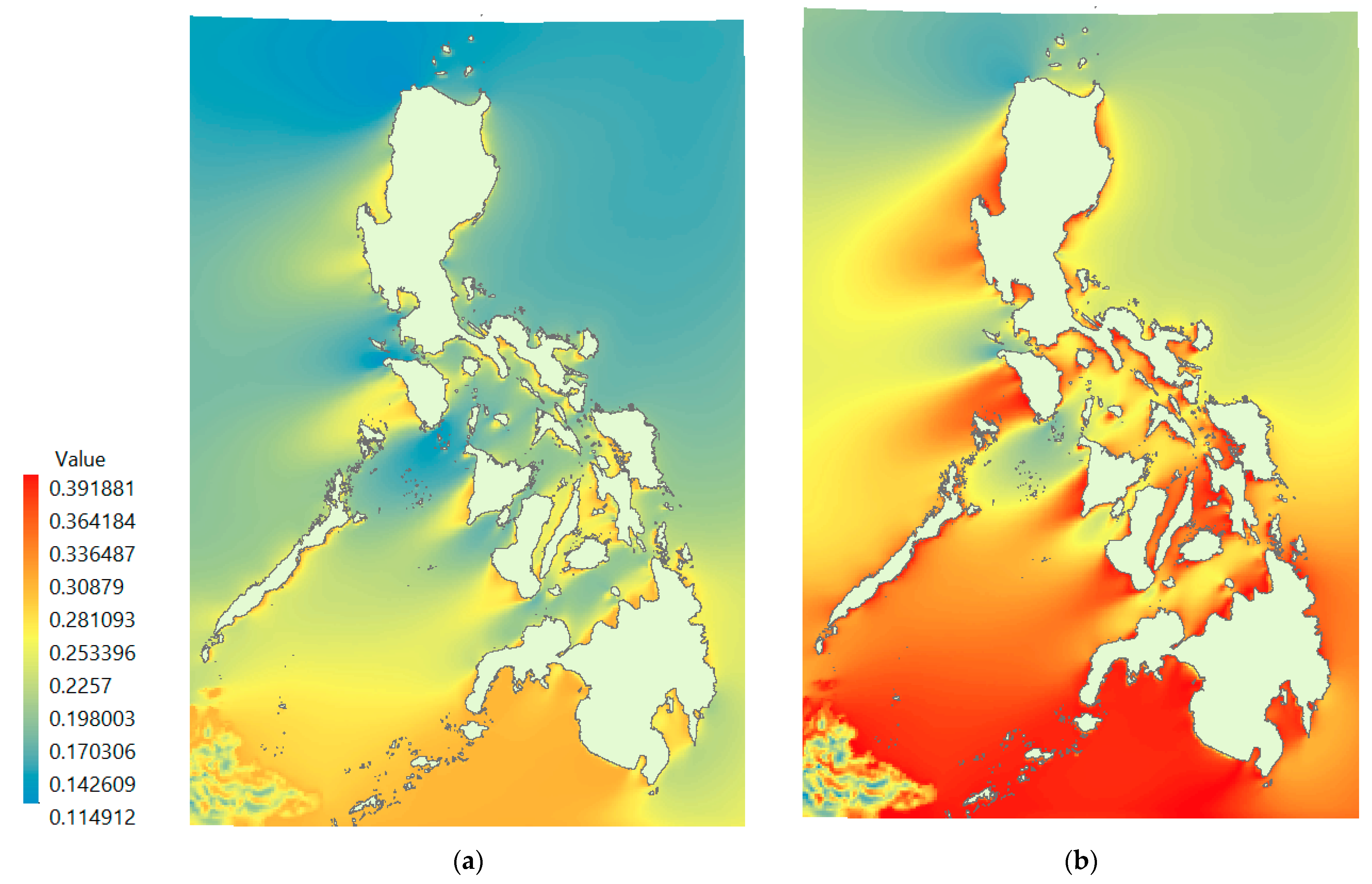
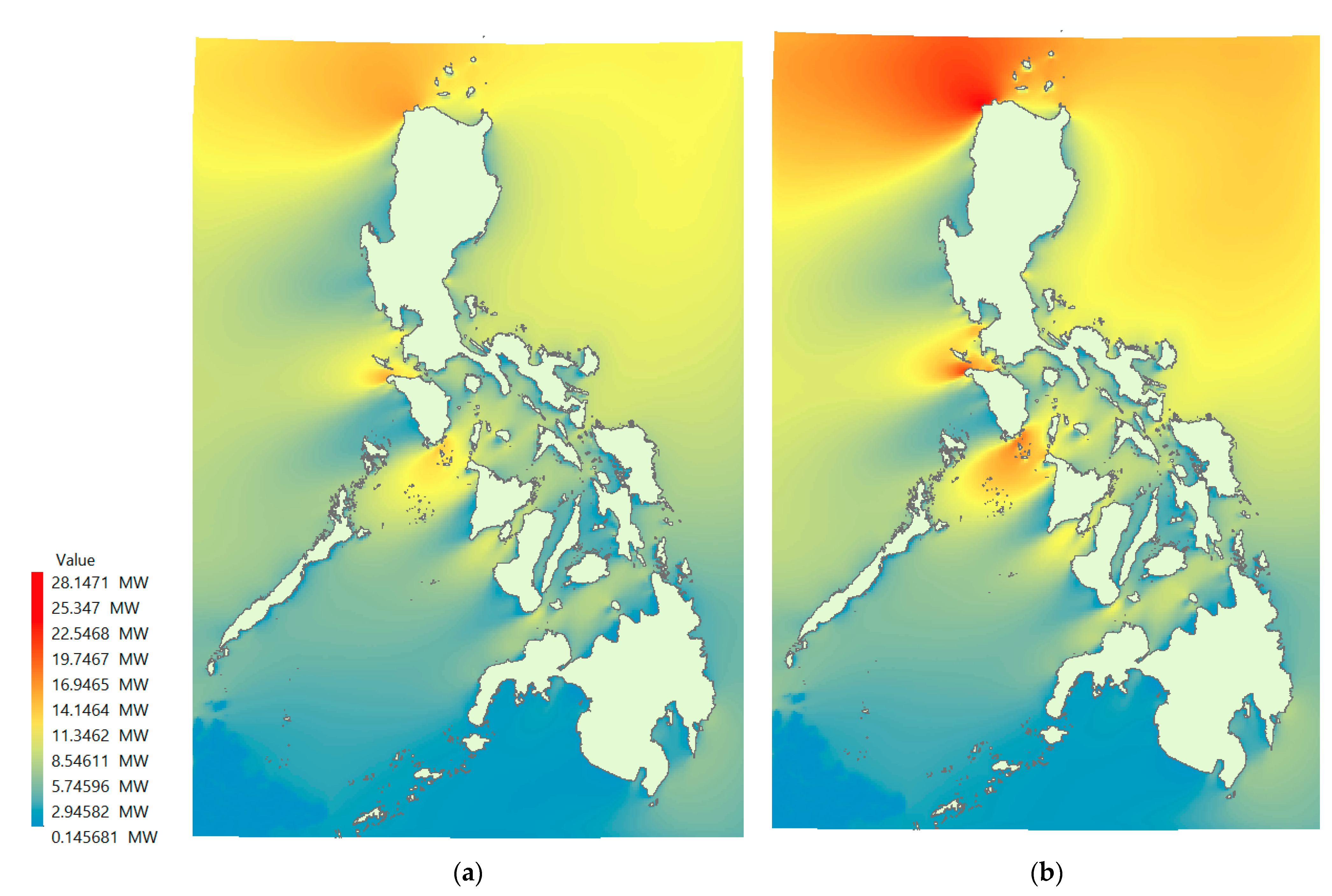
4.1. Technical Analysis
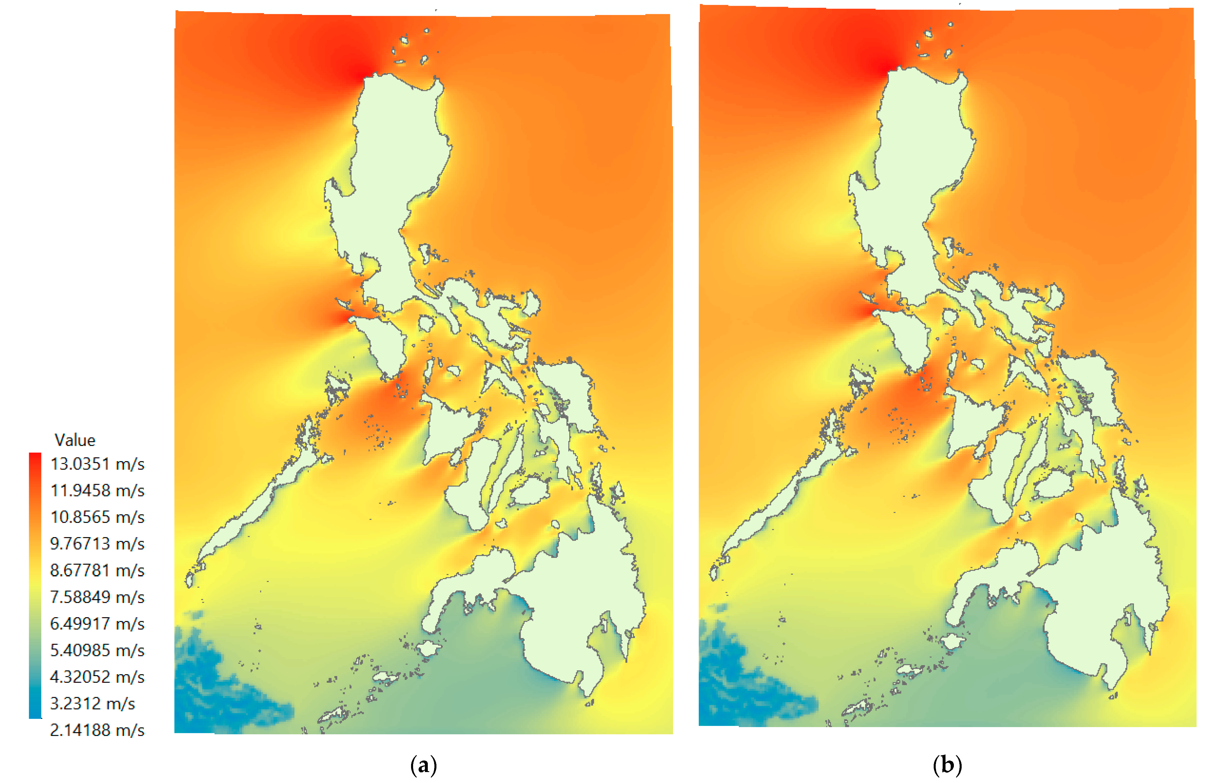
4.1.1. Wind Speed
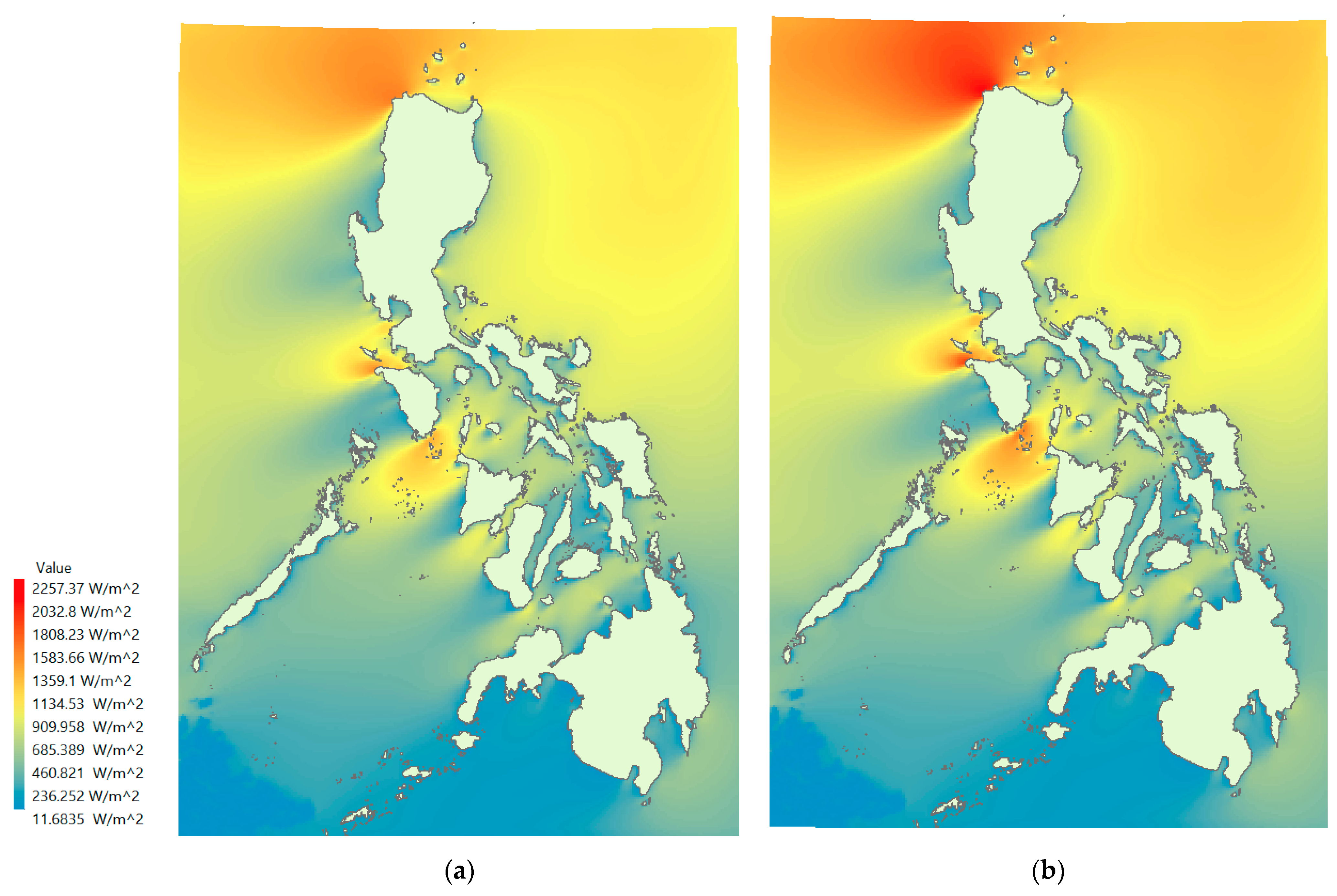
4.1.2. Wind Power Density
4.1.3. Wind Power
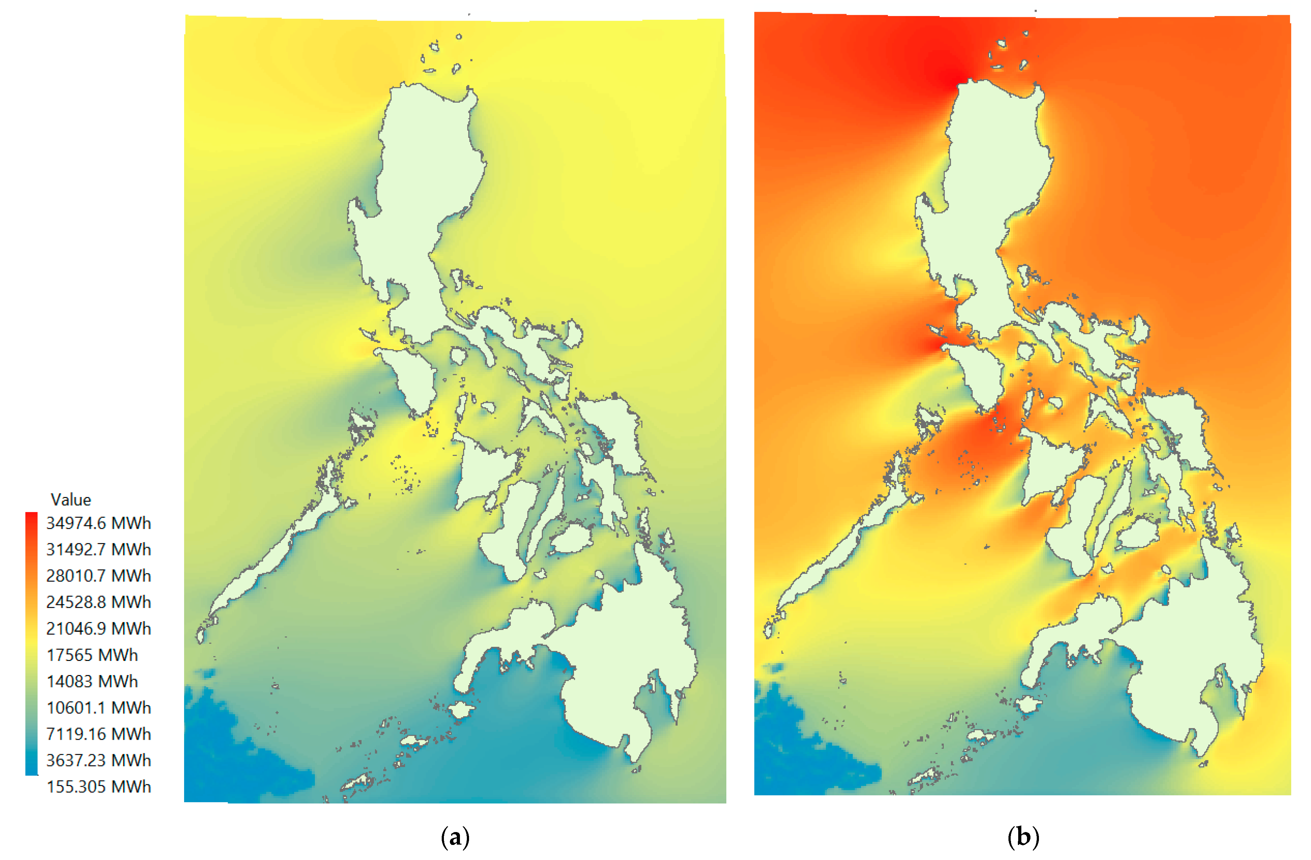
4.1.4. Annual Energy Production
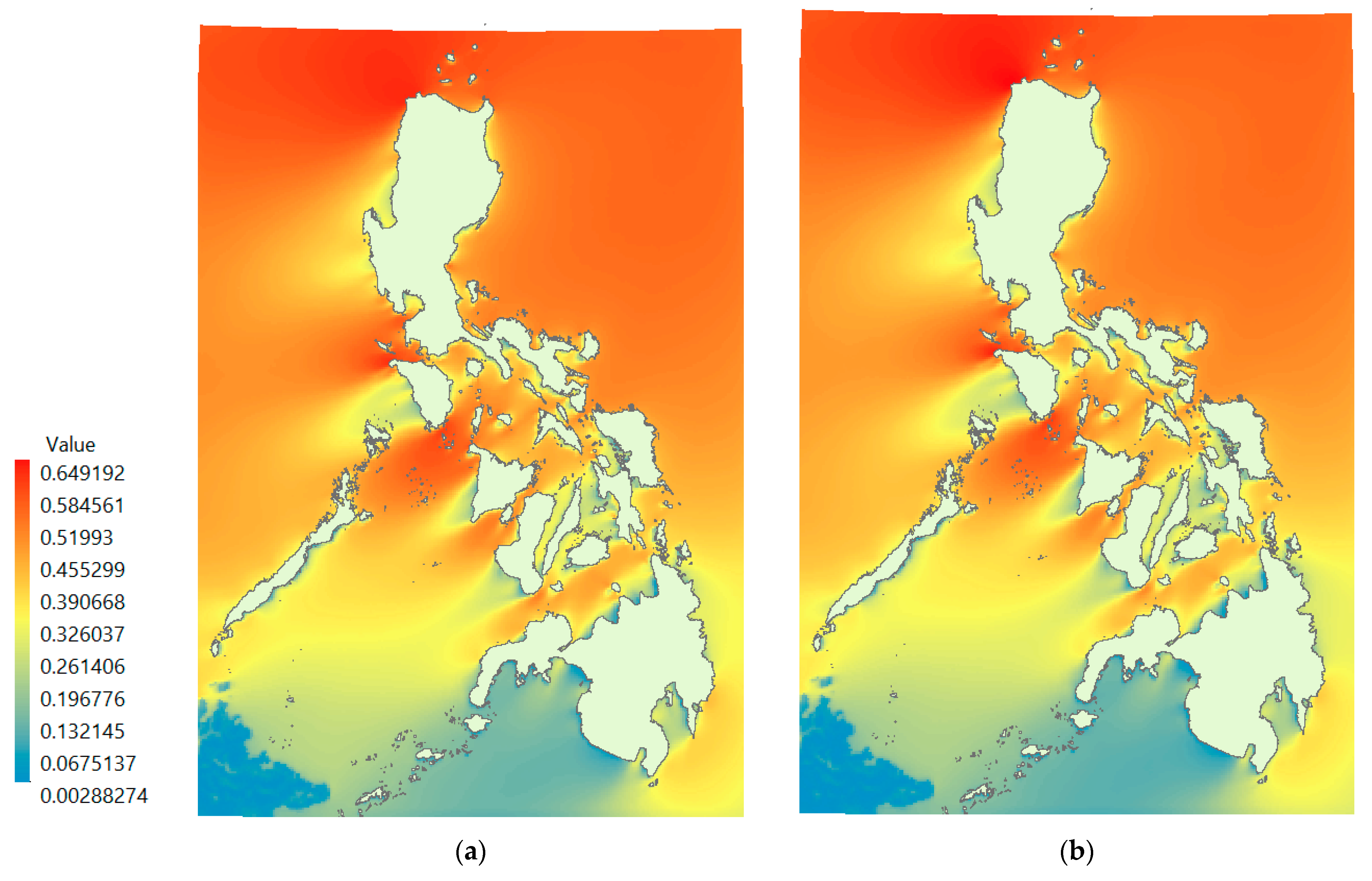
4.1.5. Capacity Factor
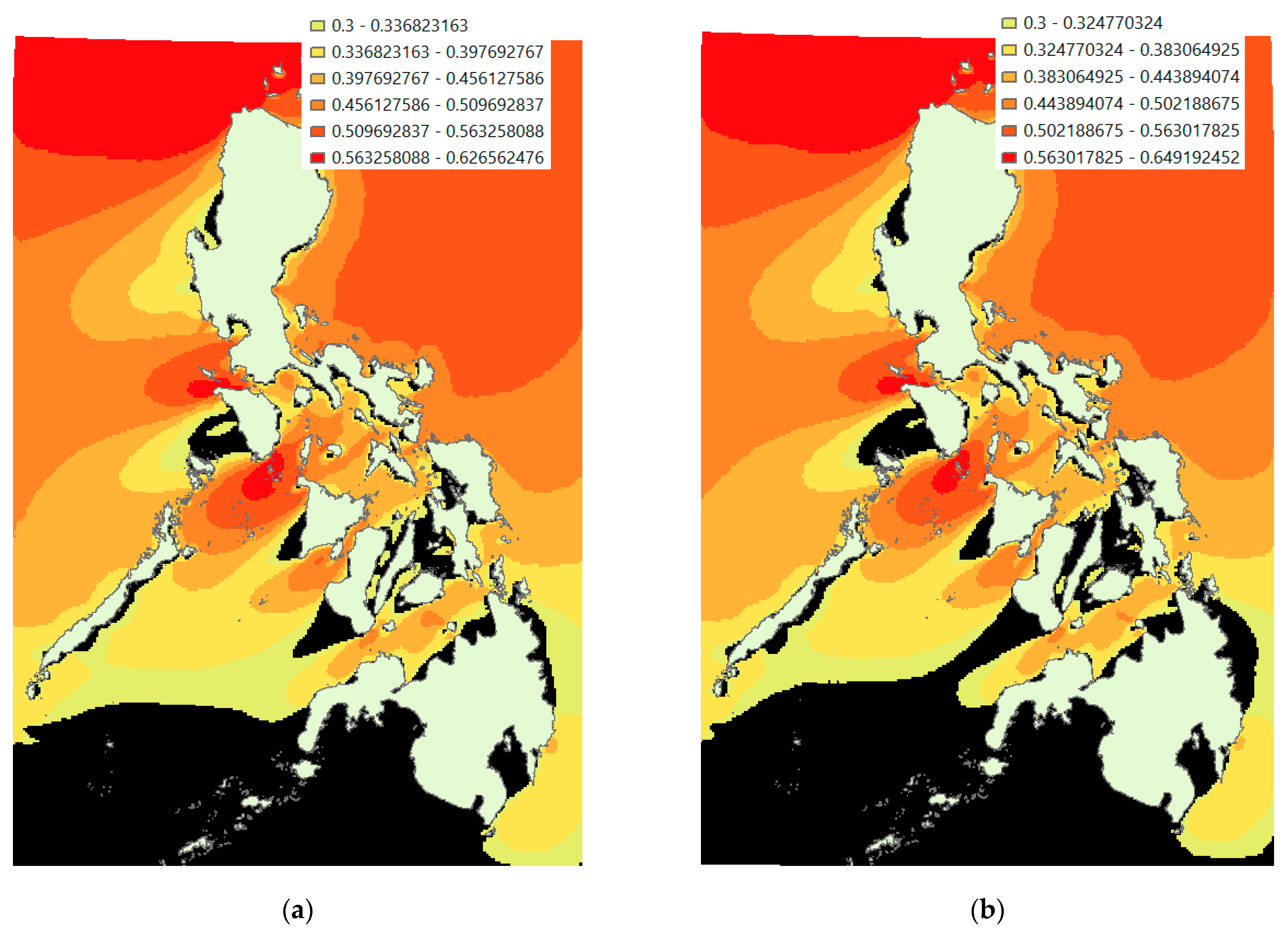
4.1.6. Performance
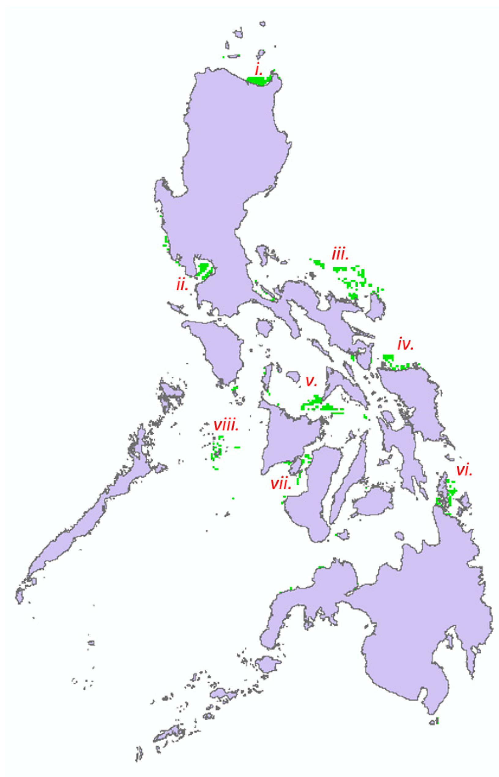
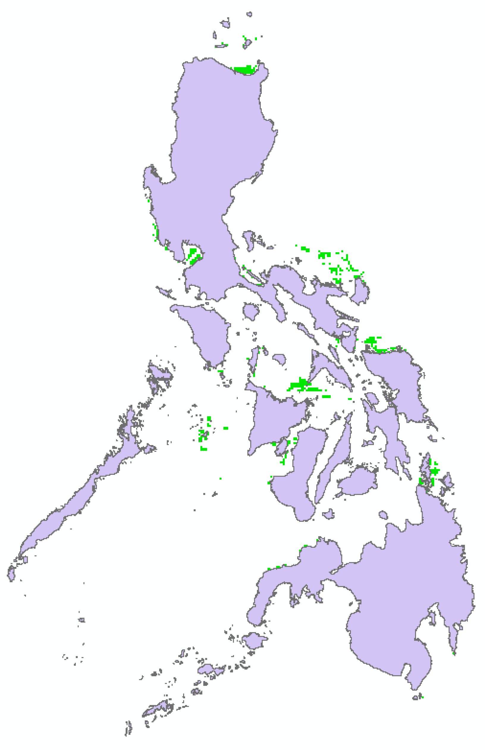
4.2. Application of Exclusion Criteria
4.3. Economic Analysis
4.3.1. Multiple Linear Regression
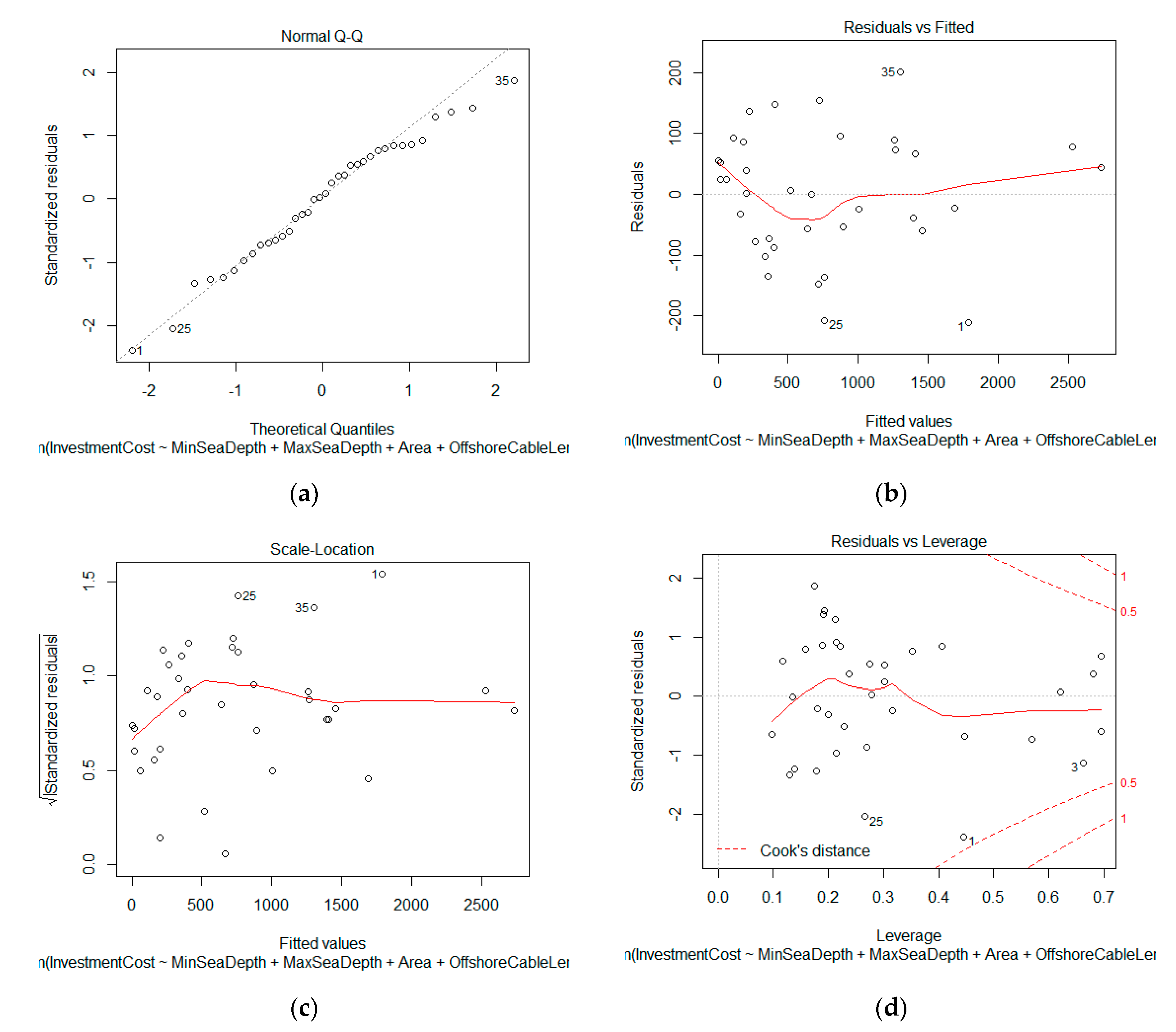
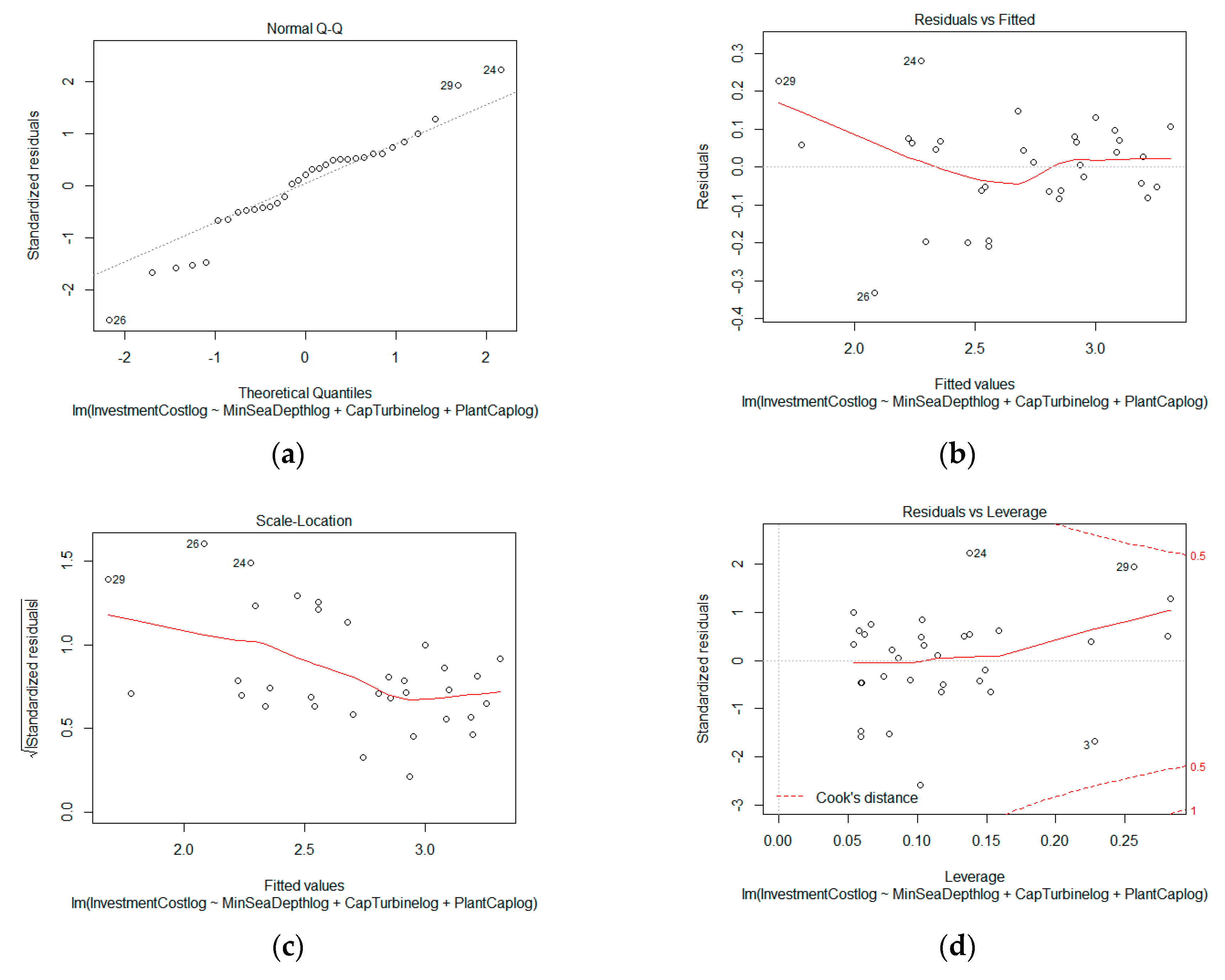
4.3.2. Regression Model Diagnostics
4.3.3. Model Selection
4.3.4. Adjusted R2
4.3.5. Investment Cost Regression Model 8
4.3.6. Checking of Investment Cost Regression Model 8
4.3.7. Selection of Investment Cost Regression Model
4.3.8. Multiple Linear Regression Model Validation
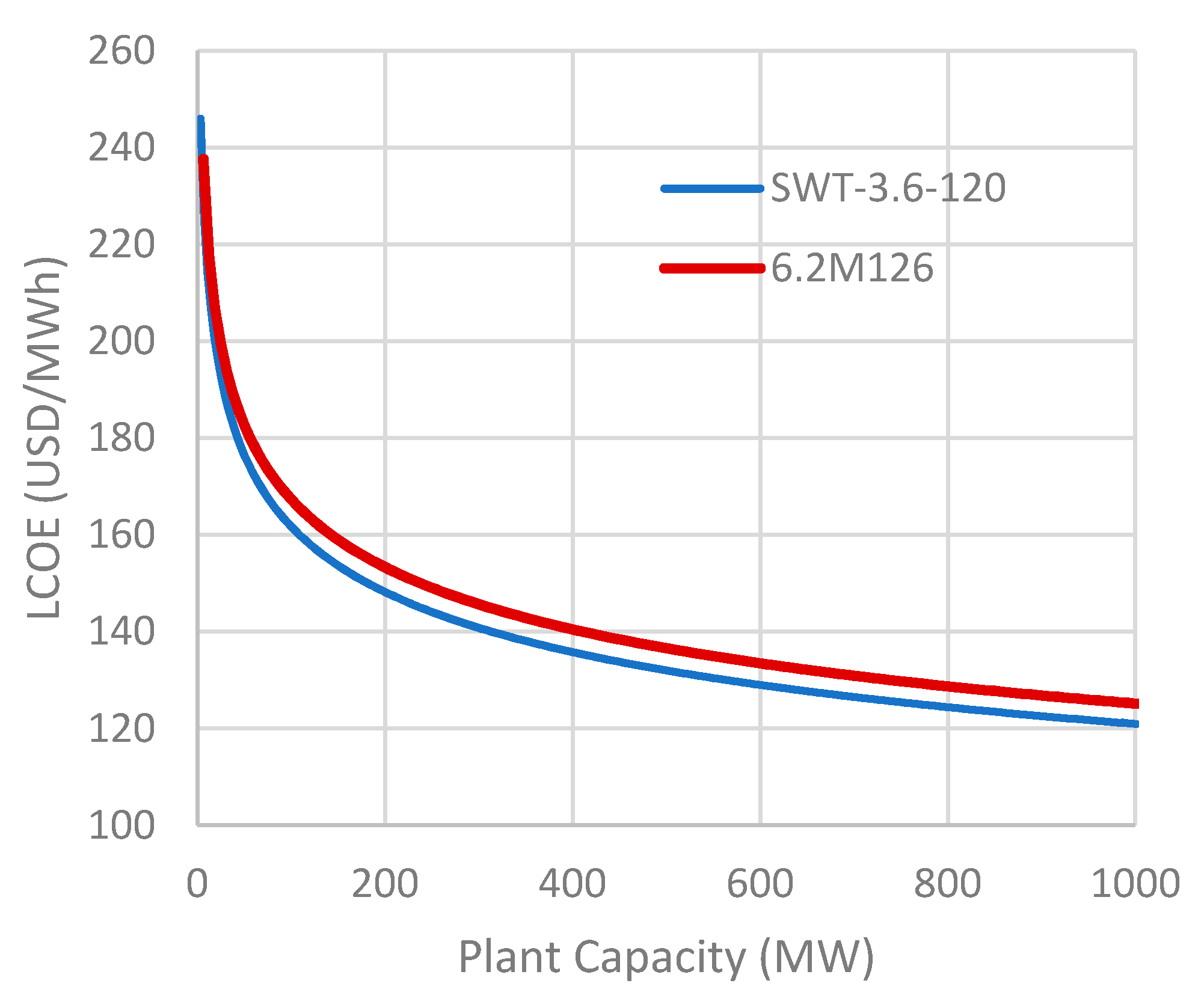
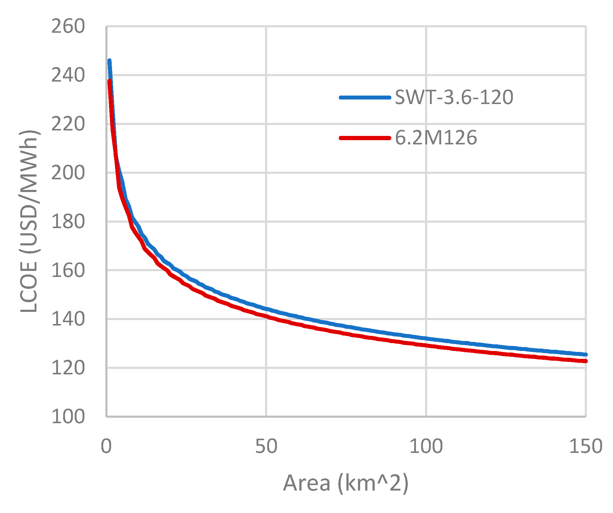
4.4. Levelized Cost of Electricity
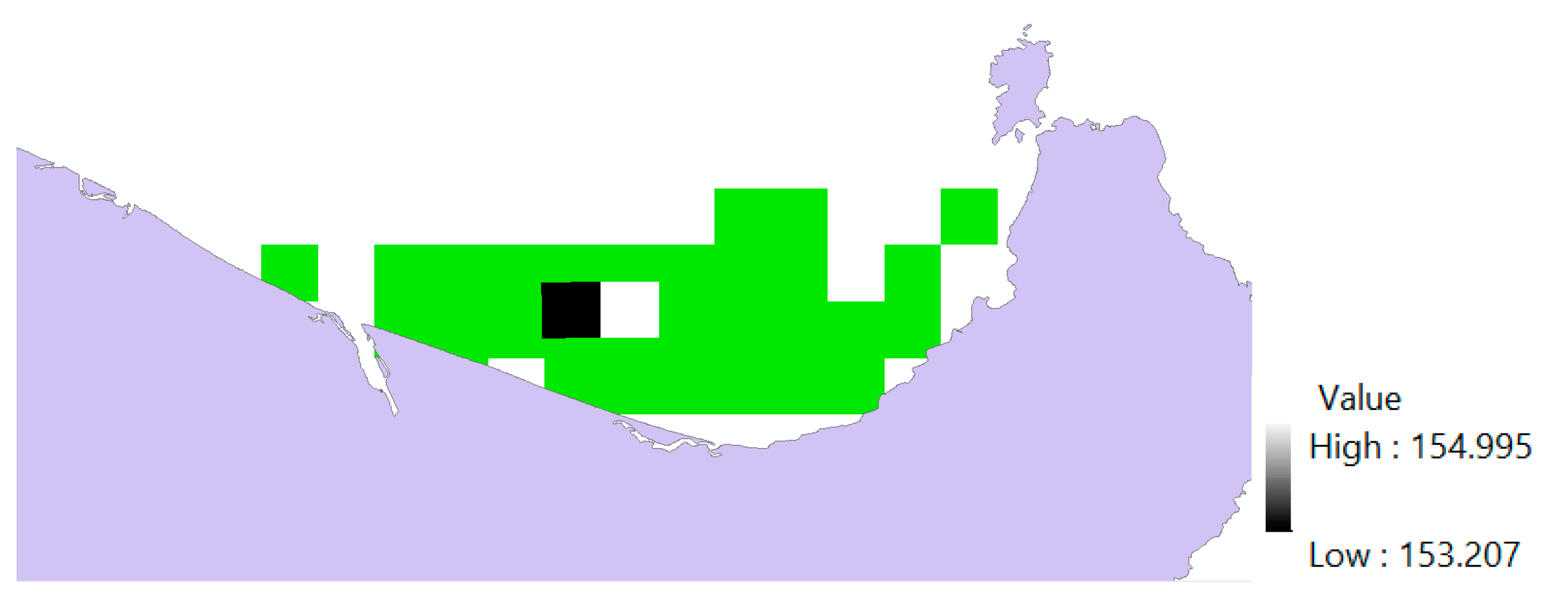
4.5. Price of Electricity
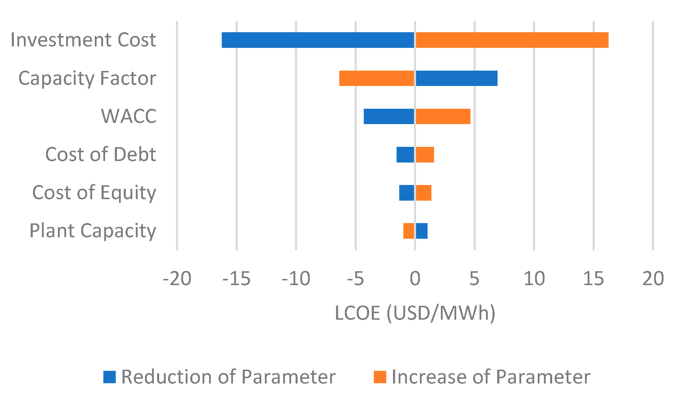
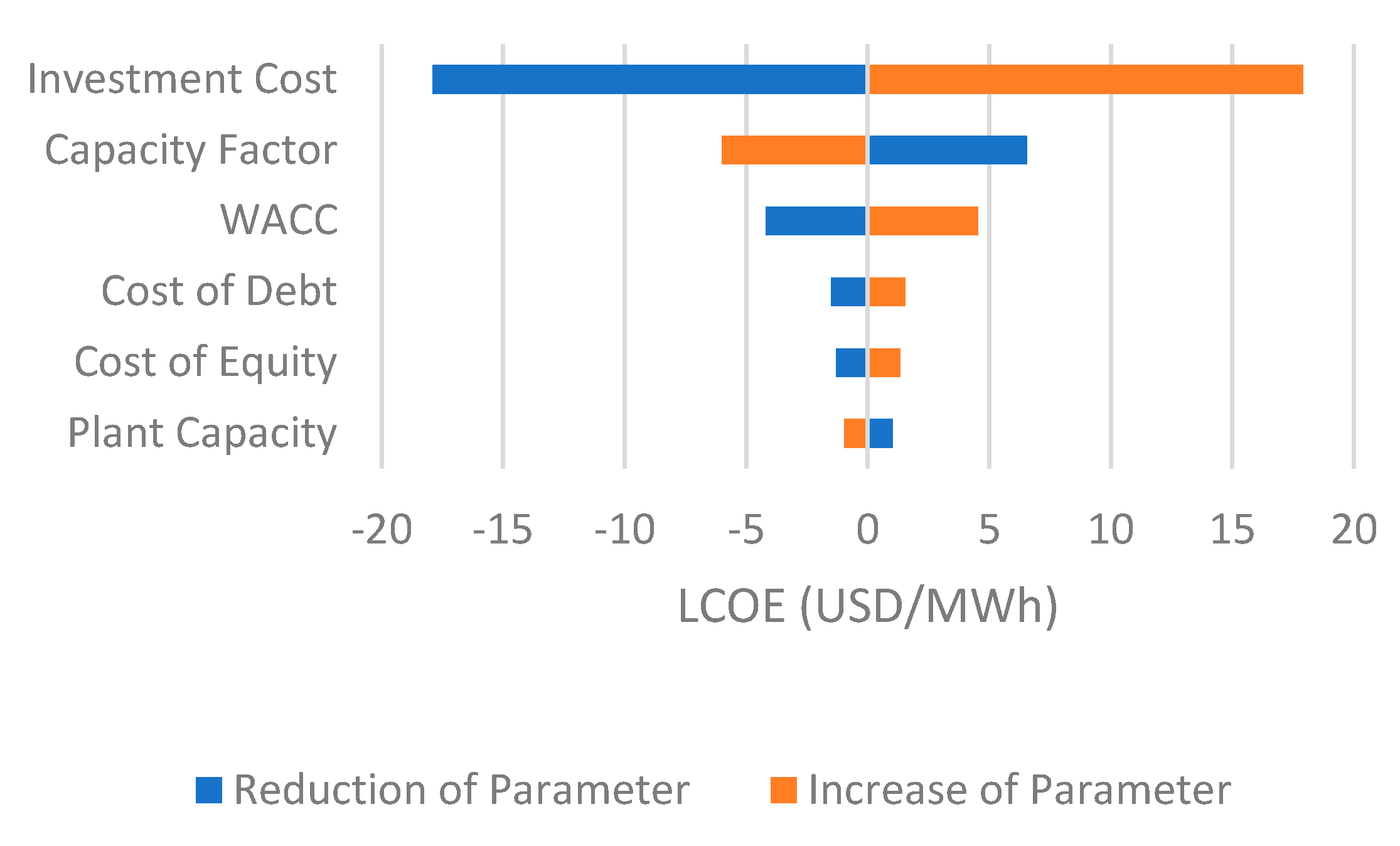
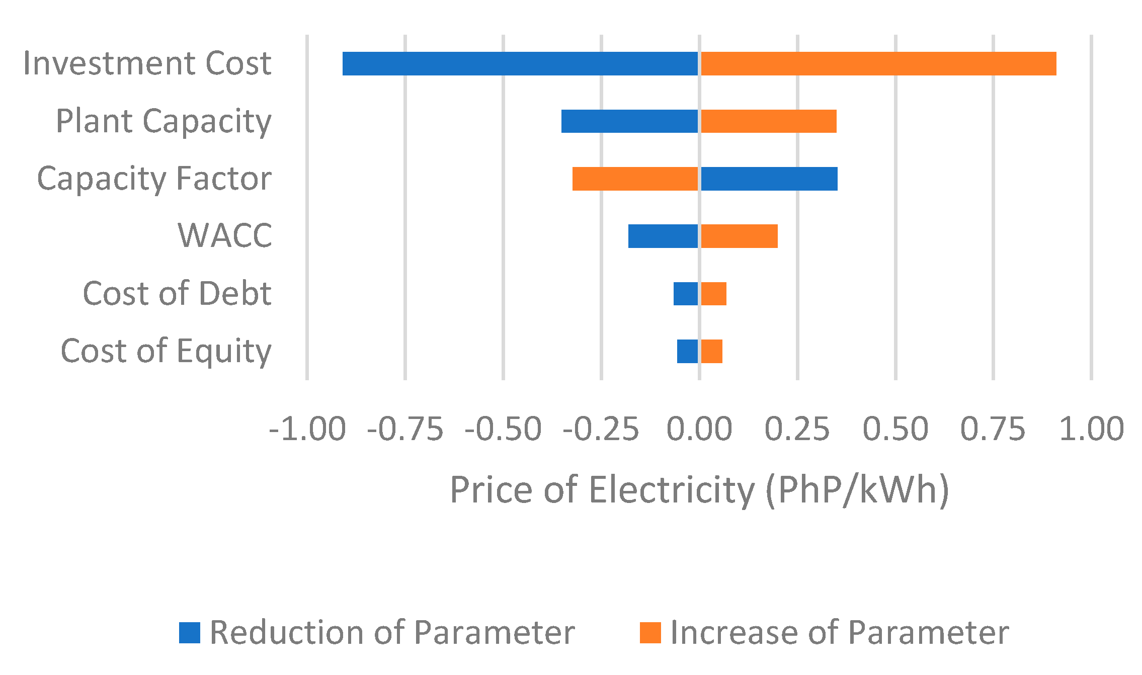
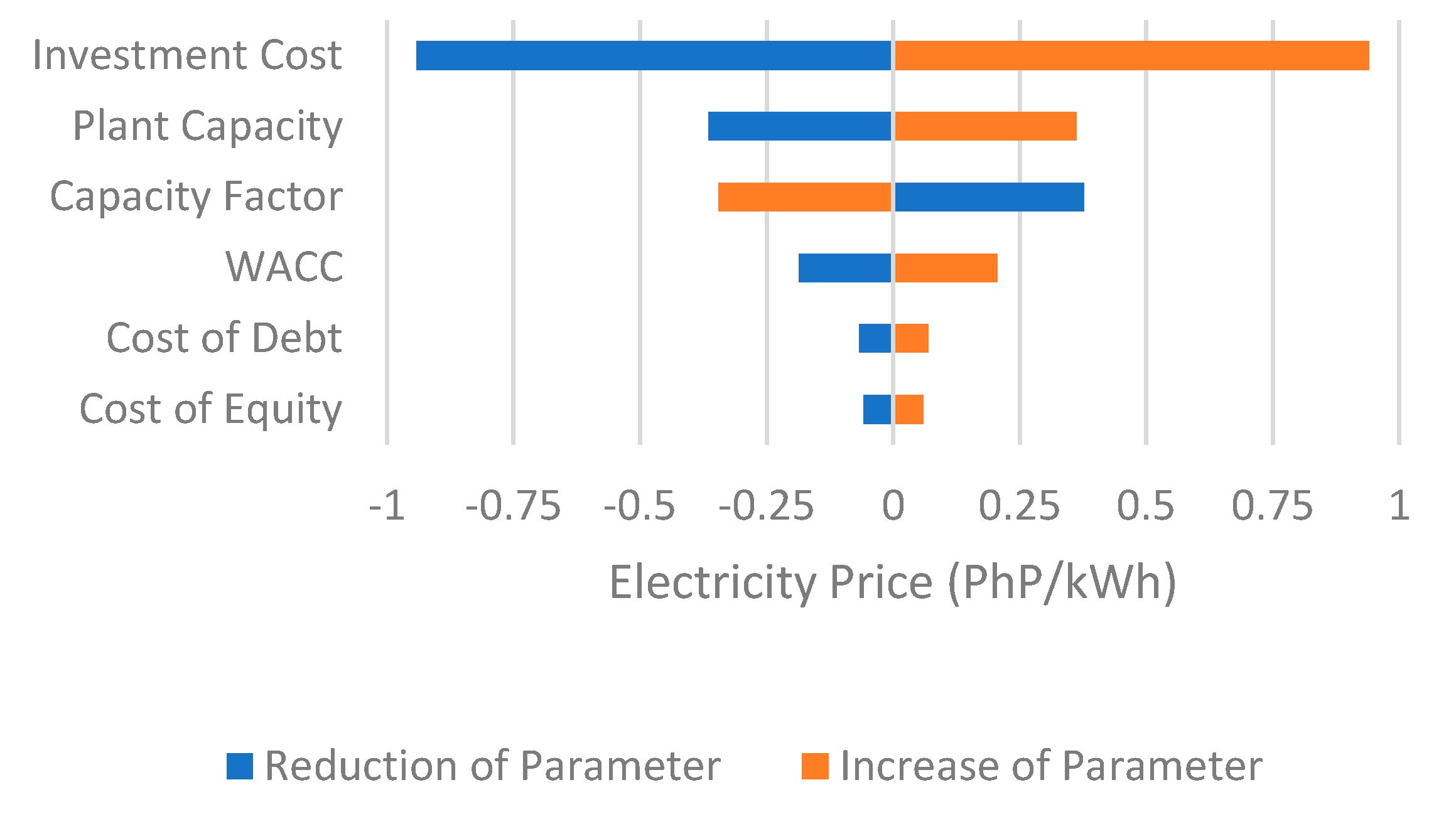
4.6. Sensitivity Analysis
5. Conclusions and Recommendations
Author Contributions
Funding
Acknowledgments
Conflicts of Interest
References
- GOV.PH. An Act Promoting the Development, Utilization and Commercialization of Renewable Energy Resources and for Other Purposes; Republic Act No. 9513; GOV.PH: Metro Manila, Philippines, 2008.
- GOV.PH. Department of Energy, Department Circular DC2009-05-0008; Rules and Regulations Implementing Republic Act 9513; GOV.PH: Metro Manila, Philippines, 2009.
- Department of Energy—Electric Power Industry Management Bureau. 2015 Philippine Power Situation Report; Department of Energy: Taguig, Philippines, 2016.
- Perveen, R.; Kishor, N.; Mohanty, S. Off-shore wind farm development: Present status and challenges. Renew. Sustain. Energy Rev. 2014, 29, 780–792. [Google Scholar] [CrossRef]
- Richts, C.; Jansen, M.; Siefert, M. Determining the Economic Value of Offshore Wind Power Plants in the Changing Energy System. Energy Procedia 2015, 80, 422–432. [Google Scholar] [CrossRef]
- Department of Energy. List of Existing Power Plants in Luzon as of June 2016; Department of Energy: Taguig, Philippines, 2016.
- Department of Energy. List of Existing Power Plants in Visayas as of June 2016; Department of Energy: Taguig, Philippines, 2016.
- Wang, S.; Wang, S. Impacts of wind energy on environment: A review. Renew. Sustain. Energy Rev. 2015, 49, 437–443. [Google Scholar] [CrossRef]
- Bakker, R.; Pedersen, E.; Van Den Berg, G.; Stewart, R.; Lok, W.; Bouma, J. Impact of wind turbine sound on annoyance, self-reported sleep disturbance and psychological distress. Sci. Total Environ. 2012, 425, 42–51. [Google Scholar] [CrossRef] [Green Version]
- Green, R.; Vasilakos, N. The economics of offshore wind. Energy Policy 2011, 39, 496–502. [Google Scholar] [CrossRef]
- Zerrahn, A. Wind Power and Externalities. Ecol. Econ. 2017, 141, 245–260. [Google Scholar] [CrossRef]
- Pineda, I.; Tardieu, P. Wind in Power 2017 Annual Combined Onshore and Offshore Wind Energy Statistics; WindEurope: Brussels, Belgium, 2018. [Google Scholar]
- Rodrigues, S.; Restrepo, C.; Kontos, E.; Teixeira Pinto, R.; Bauer, P. Trends of offshore wind projects. Renew. Sustain. Energy Rev. 2015, 49, 1114–1135. [Google Scholar] [CrossRef]
- Shi, W.; Park, H.; Chung, C.; Kim, Y. Comparison of Dynamic Response of Monopile, Tripod and Jacket Foundation System for a 5-MW Wind Turbine. In Twenty-First (2011) International Offshore and Polar Engineering Conference; International Society of Offshore and Polar Engineers: Maui, Hawaii, 2011. [Google Scholar]
- Arapogianni, A.; Genachte, A. Deep Water—The Next Step for Offshore Wind Energy; European Wind Energy Association: Brussels, Belgium, 2013. [Google Scholar]
- Mattar, C.; Guzmán-Ibarra, M. A techno-economic assessment of offshore wind energy in Chile. Energy 2017, 133, 191–205. [Google Scholar] [CrossRef]
- Nagababu, G.; Kachhwaha, S.; Naidu, N.; Savsani, V. Application of reanalysis data to estimate offshore wind potential in EEZ of India based on marine ecosystem considerations. Energy 2017, 118, 622–631. [Google Scholar] [CrossRef]
- Khraiwish Dalabeeh, A. Techno-economic analysis of wind power generation for selected locations in Jordan. Renew. Energy 2017, 101, 1369–1378. [Google Scholar] [CrossRef]
- Schweizer, J.; Antonini, A.; Govoni, L.; Gottardi, G.; Archetti, R.; Supino, E.; Berretta, C.; Casadei, C.; Ozzi, C. Investigating the potential and feasibility of an offshore wind farm in the Northern Adriatic Sea. Appl. Energy 2016, 177, 449–463. [Google Scholar] [CrossRef]
- Cavazzi, S.; Dutton, A. An Offshore Wind Energy Geographic Information System (OWE-GIS) for assessment of the UK’s offshore wind energy potential. Renew. Energy 2016, 87, 212–228. [Google Scholar] [CrossRef]
- Mahdy, M.; Bahaj, A. Multi criteria decision analysis for offshore wind energy potential in Egypt. Renew. Energy 2018, 118, 278–289. [Google Scholar] [CrossRef]
- Hornyak, T. Here’s What To Takes To Lay Google’s 9000 km Undersea Cable. 2015. Available online: https://www.infoworld.com/article/2947900/networking/heres-what-to-takes-to-lay-googles-9000km-undersea-cable.html (accessed on 11 April 2018).
- Submarine Cable Map. 2017. Available online: https://www.submarinecablemap.com/ (accessed on 15 April 2018).
- Crevoisier, T. Philippines, Operational Ferry Routes. 2014. Available online: https://geonode.wfp.org/layers/geonode:phl_trs_waterways_wfp#more (accessed on 11 May 2018).
- GOV.PH. An Act Providing for the Establishment and Management of National Integrated Protected Areas System, Defining Its Scope and Coverage, and for Other Purposes; Republic Act No. 7586; GOV.PH: Metro Manila, Philippines, 1992.
- UNEP-WCMC. Protected Area Profile for Philippines from the World Database of Protected Areas. 2018. Available online: https://www.protectedplanet.net/country/PH (accessed on 15 April 2018).
- Weeks, R.; Russ, G.; Alcala, A.; White, A. Effectiveness of Marine Protected Areas in the Philippines for Biodiversity Conservation. Conserv. Biol. 2010, 24, 531–540. [Google Scholar] [CrossRef]
- Cabral, R.; Geronimo, R. How important are coral reefs to food security in the Philippines? Diving deeper than national aggregates and averages. Mar. Policy 2018, 91, 136–141. [Google Scholar] [CrossRef]
- Gomez, E.; Aliño, P.; Yap, H.; Licuanan, W. A review of the status of Philippine reefs. Mar. Pollut. Bull. 1994, 29, 62–68. [Google Scholar] [CrossRef]
- ReefBase. A Global Information System for Coral Reefs. 2018. Available online: http://www.reefbase.org (accessed on 1 May 2018).
- 5th Philippine Energy Contracting Round (PERC5). 5Th Philippine Energy Contracting Round Petroleum Areas for Offer Figures and Maps. 2014. Available online: https://www.doe.gov.ph/figures-and-maps-petroleum (accessed on 15 May 2018).
- Philippine Bathymetry Grid. General Bathymetric Chart of the Oceans (GEBCO). 2018. Available online: https://www.gebco.net/ (accessed on 20 April 2018).
- Philippine Transmission Lines. Renewable Energy Data Explorer, National Renewable Energy Laboratory. 2018. Available online: https://www.re-explorer.org/ (accessed on 27 March 2018).
- Worsnop, R.; Lundquist, J.; Bryan, G.; Damiani, R.; Musial, W. Gusts and shear within hurricane eyewalls can exceed offshore wind turbine design standards. Geophys. Res. Lett. 2017, 44, 6413–6420. [Google Scholar] [CrossRef] [Green Version]
- Philippines: Hazard Profile. UN Office for the Coordination of Humanitarian Affairs. 2017. Available online: https://reliefweb.int/map/philippines/philippines-hazard-profile-jan-2017 (accessed on 1 March 2018).
- Black, M.; Willoughby, H. The Concentric Eyewall Cycle of Hurricane Gilbert. Mon. Weather Rev. 1992, 120, 947–957. [Google Scholar] [CrossRef] [Green Version]
- Takagi, H.; Wu, W. Maximum wind radius estimated by the 50 kt radius: Improvement of storm surge forecasting over the western North Pacific. Nat. Hazards Earth Syst. Sci. 2016, 16, 705–717. [Google Scholar] [CrossRef] [Green Version]
- Matsunobu, T.; Inoue, S.; Tsuji, Y.; Yoshida, K.; Komatsuzaki, M. Seismic Design of Offshore Wind Turbine Withstands Great East Japan Earthquake and Tsunami. J. Energy Power Eng. 2014, 8, 2039–2044. [Google Scholar]
- Truelsen, C. Offshore Wind Turbines Must Withstand Typhoons and Earthquakes in Taiwan. Available online: https://www.niras.com/projects/offshore-jacket-design/ (accessed on 10 April 2018).
- Chiaradonna, A.; Tropeano, G.; Donofrio, A.; Silvestri, F. Interpreting the deformation phenomena of a levee damaged during the 2012 Emilia earthquake. Soil Dyn. Earthq. Eng. 2019, 124, 389–398. [Google Scholar] [CrossRef]
- Bird, L.; Cochran, J.; Wang, X. Wind and Solar Energy Curtailment: Experience and Practices in the United States; NREL/TP-6A20-60983; National Renewable Energy Laboratory: Golden, CO, USA, 2014.
- Bird, L.; Lew, D.; Milligan, M.; Carlini, E.; Estanqueiro, A.; Flynn, D.; Gomez-Lazaro, E.; Holttinen, H.; Menemenlis, N.; Orths, A.; et al. Wind and solar energy curtailment: A review of international experience. Renew. Sustain. Energy Rev. 2016, 65, 577–586. [Google Scholar] [CrossRef] [Green Version]
- Ang, M.R.C.O.; Blanco, A.C. Philippine Renewable Energy Resource Mapping from LiDAR Surveys (REMap) Project Terminal Report; UP TCAGP: Quezon City, Philippines, 2017. [Google Scholar]
- Murthy, K.; Rahi, O. A comprehensive review of wind resource assessment. Renew. Sustain. Energy Rev. 2017, 72, 1320–1342. [Google Scholar] [CrossRef]
- Celik, A. A statistical analysis of wind power density based on the Weibull and Rayleigh models at the southern region of Turkey. Renew. Energy 2004, 29, 593–604. [Google Scholar] [CrossRef]
- Siemens AG. Thoroughly Tested, Utterly Reliable Siemens Wind Turbine SWT-3.6-120. 2011. Available online: https://www.siemens.com.tr/i/Assets/Enerji/yenilenebilir_enerji/E50001-W310-A169-X-4A00_WS_SWT_3-6_120_US.pdf (accessed on 16 March 2018).
- Senvion GmbH. 3.2M126 Wind Turbine 6.2MW. 2017. Available online: https://www.senvion.com/global/en/products-services/wind-turbines/6xm/62m126/ (accessed on 17 March 2018).
- Tegen, S.; Lantz, E.; Hand, M.; Maples, B.; Smith, A.; Schwabe, P. 2011 Cost of Wind Energy Review; NREL/TP-5000-56266; National Renewable Energy Laboratory: Golden, CO, USA, 2013.
- Nagababu, G.; Kachhwaha, S.; Savsani, V. Estimation of technical and economic potential of offshore wind along the coast of India. Energy 2017, 138, 79–91. [Google Scholar] [CrossRef]
- Sheridan, B.; Baker, S.; Pearre, N.; Firestone, J.; Kempton, W. Calculating the offshore wind power resource: Robust assessment methods applied to the U.S. Atlantic Coast. Renew. Energy 2012, 43, 224–233. [Google Scholar] [CrossRef]
- Gonzalez-Rodriguez, A. Review of offshore wind farm cost components. Energy Sustain. Dev. 2017, 37, 10–19. [Google Scholar] [CrossRef]
- Li, D.; Geyer, B.; Bisling, P. A model-based climatology analysis of wind power resources at 100-m height over the Bohai Sea and the Yellow Sea. Appl. Energy 2016, 179, 575–589. [Google Scholar] [CrossRef]
- Schwanitz, V.; Wierling, A. Offshore wind investments—Realism about cost developments is necessary. Energy 2016, 106, 170–181. [Google Scholar] [CrossRef]
- Montgomery, D.; Runger, G. Applied Statistics and Probability for Engineers, 3rd ed.; John Wiley & Sons, Inc.: Danvers, MA, USA, 2003. [Google Scholar]
- De Myttenaere, A.; Golden, B.; Le Grand, B.; Rossi, F. Mean Absolute Percentage Error for regression models. Neurocomputing 2016, 192, 38–48. [Google Scholar] [CrossRef] [Green Version]
- Osborne, J.W.; Waters, E. Four assumptions of multiple regression that researchers should always test. Pract. Assess. Res. Eval. 2002, 8, 2. [Google Scholar]
- Kim, B. Understanding Diagnostic Plots for Linear Regression Analysis University of Virginia Library Research Data Services + Sciences. Data.library.virginia.edu. 2015. Available online: https://data.library.virginia.edu/diagnostic-plots/ (accessed on 3 May 2018).
- Ioannou, A.; Angus, A.; Brennan, F. Stochastic Prediction of Offshore Wind Farm LCOE through an Integrated Cost Model. Energy Procedia 2017, 107, 383–389. [Google Scholar] [CrossRef]
- Möller, B.; Hong, L.; Lonsing, R.; Hvelplund, F. Evaluation of offshore wind resources by scale of development. Energy 2012, 48, 314–322. [Google Scholar] [CrossRef] [Green Version]
- Cohen, J. Statistical Power Analysis for the Behavioral Sciences, 2nd ed.; Erlbaum: Hillsdale, NJ, USA, 1987. [Google Scholar]
- Mone, C.; Hand, M.; Bolinger, M.; Rand, J.; Heimiller, D.; Ho, J. 2015 Cost of Wind Energy Review; NREL/TP-6A20-66861; National Renewable Energy Laboratory: Golden, CO, USA, 2017.


| Name | Individual Variables | Variable Removed | VIF |
|---|---|---|---|
| Model 8 | MinSeaDepth + Area + OffshoreCableLength + OnshoreCableLength + PortDistance + CapTurbine + PlantCap | MaxSeaDepth, NumTurbine, lnterArrayCableLength | MinSeaDepth = 1.966903, Area = 3.014808, OffshoreCableLength = 2.154003, OnshoreCablelength = 1.248556, PortDistance = 1.377031, CapTurbine = 1.402520, PlantCap = 3.646495 |
| Model 9 | MaxSeaDepth + Area + OffshoreCablelength + OnshoreCablelength + PortDistance + CapTurbine + PlantCap | MinSeaDepth, NumTurbine, lnterArrayCablelength | MaxSeaDepth = 2.474813, Area = 3.207744, OffshoreCablelength = 2.009005, OnshoreCableLength = 1.229875, PortDistance = 1.493217, CapTurbine = 1.647750, PlantCap = 3.860488 |
| Model 16 | MinSeaDepth + OffshoreCablelength + OnshoreCablelength + PortDistance + CapTurbine + PlantCap | MaxSeaDepth, Area, lnterArrayCablelength, NumTurbine | MinSeaDepth = 1.966185, OffshoreCablelength = 2.113326, OnshoreCablelength = 1.229009, PortDistance = 1.363429, CapTurbine = 1.402447, PlantCap = 1.558588 |
| Model 17 | MaxSeaDepth + OffshoreCablelength + OnshoreCablelength + PortDistance + Cap Turbine + PlantCap | MinSeaDepth, Area, lnterArrayCablelength, NumTurbine | MaxSea Depth = 2.325112, OffshoreCableLength = 2.008671, OnshoreCablelength = 1.210969, PortDistance = 1.440038, CapTurbine = 1.622965, PlantCap = 1.486171 |
| Model 21 | MinSeaDepth + Area + OffshoreCableLength + OnshoreCablelength + PortDistance + NumTurbine + CapTurbine | PlantCap, MaxSeaDepth, lnterArrayCableLength | MinSeaDepth = 1.948631, Area = 2.866016, OffshoreCableLength = 1.920793, OnshoreCablelength = 1.247374, PortDistance = 1.370884, NumTurbine = 3.566499, CapTurbine = 1.615025 |
| Model 22 | MaxSeaDepth +Area+ OffshoreCablelength + OnshoreCablelength + PortDistance + NumTurbine + CapTurbine | PlantCap, MinSeaDepth, lnterArrayCablelength | MaxSeaDepth = 2.422104, Area = 2.994082, OffshoreCablelength = 1.945860, OnshoreCablelength = 1.229641, PortDistance = 1.498961, NumTurbine = 3.730028, CapTurbine = 2.030133 |
| Model 25 | MinSeaDepth + OffshoreCablelength + OnshoreCablelength + PortDistance + NumTurbine + CapTurbine | PlantCap, MaxSeaDepth, Area, lnterArrayCablelength | MinSeaDepth = 1.943687, OffshoreCablelength = 1.920234, OnshoreCableLength = 1.224317, PortDistance = 1.344159, NumTurbine = 1.603537, Cap Turbine = 1.528544 |
| Model 26 | MaxSeaDepth + OffshoreCablelength + OnshoreCablelength + PortDistance + NumTurbine + CapTurbine | PlantCap, MinSeaDepth, Area, lnterArrayCablelength | MaxSeaDepth = 2.312621, OffshoreCablelength = 1.932499, OnshoreCablelength = 1.208195, PortDistance = 1.436073, NumTurbine = 1.538419, Cap Turbine = 1.841882 |
| Name | Individual Variables | Variable Removed | Multiple R2 | Adj. R2 |
|---|---|---|---|---|
| Model 8 | MinSeaDepth + Area + OffshoreCablelength + OnshoreCablelength + PortDistance + CapTurbine + PlantCap | MaxSeaDepth, NumTurbine, lnterArrayCablelength | 97.40% | 96.75% |
| Model 9 | MaxSeaDepth + Area + OffshoreCablelength + OnshoreCablelength + PortDistance + CapTurbine + PlantCap | MinSeaDepth, NumTurbine, lnterArrayCablelength | 97.24% | 96.55% |
| Model 16 | MinSeaDepth + OffshoreCablelength + OnshoreCablelength + PortDistance + CapTurbine+ PIantcap | MaxSeaDepth, Area, lnterArrayCablelength, NumTurbine | 96.42% | 95.68% |
| Model 17 | MaxSeaDepth + OffshoreCablelength + OnshoreCablelength + PortDistance + CapTurbine + PlantCap | MinSeaDepth, Area, lnterArrayCablelength, NumTurbine | 96.34% | 95.59% |
| Model 21 | MinSeaDepth + Area + OffshoreCablelength + OnshoreCablelength + PortDistance + NumTurbine + CapTurbine | PlantCap, MaxSeaDepth, lnterArrayCablelength | 91.80% | 89.75% |
| Model 22 | MaxSeaDepth +Area+ OffshoreCablelength + OnshoreCablelength + PortDistance + NumTurbine+ CapTurbine | Plant Cap, MinSeaDepth, lnterArrayCablelength | 91.97% | 89.96% |
| Model 25 | MinSeaDepth + OffshoreCablelength + OnshoreCablelength + PortDistance + NumTurbine + CapTurbine | PlantCap, MaxSeaDepth, Area, lnterArrayCablelength | 91.61% | 89.87% |
| Model 26 | MaxSeaDepth + OffshoreCablelength + OnshoreCablelength + PortDistance + NumTurbine + CapTurbine | PlantCap, MinSeaDepth, Area, lnterArrayCablelength | 91.85% | 90.16% |
| Actual Investment Cost (Million USD) | Predicted Investment Cost (Million USD) | Residuals | MAPE | |
|---|---|---|---|---|
| 1 | 1155.0303 | 1272.5352 | −117.504902 | 0.10173318 |
| 2 | 1610.5574 | 1636.7401 | −26.182712 | 0.01625693 |
| 3 | 1155.0303 | 1272.5352 | −117.504902 | 0.10173318 |
| 4 | 1443.7878 | 1302.7241 | 141.063756 | 0.09770394 |
| 5 | 2079.0545 | 1988.9850 | 90.069423 | 0.04332230 |
| 6 | 2485.6456 | 2534.3208 | −48.675219 | 0.01958253 |
| 7 | 1389.2856 | 1287.8844 | 101.401244 | 0.07298805 |
| 8 | 463.2340 | 334.1906 | 129.043308 | 0.27857048 |
| 9 | 1501.5393 | 1315.9762 | 185.563161 | 0.12358195 |
| 10 | 1355.8067 | 1331.0228 | 24.783887 | 0.01827981 |
| 11 | 1039.5272 | 996.5151 | 43.012121 | 0.04137662 |
| 12 | 2146.6939 | 1997.6728 | 149.021163 | 0.06941891 |
| 13 | 784.7990 | 717.1558 | 67.643246 | 0.08619180 |
| 14 | 740.0445 | 826.3828 | −86.338284 | 0.11666634 |
| 15 | 1006.9377 | 922.6834 | 84.254318 | 0.08367381 |
| 16 | 578.7908 | 477.7106 | 101.080216 | 0.17464032 |
| 17 | 415.9957 | 424.3203 | −8.324543 | 0.02001113 |
| 18 | 297.5603 | 401.2918 | −103.731481 | 0.34860655 |
| 19 | 1030.7567 | 753.9011 | 276.855596 | 0.26859451 |
| 20 | 517.0838 | 606.1924 | −89.108637 | 0.17232921 |
| 21 | 3163.5490 | 2602.6829 | 560.866112 | 0.17729016 |
| 22 | 492.4285 | 577.0530 | −84.624516 | 0.17185138 |
| 23 | 458.1789 | 479.7112 | −21.532298 | 0.04699540 |
| 24 | 898.0267 | 836.7780 | 61.248712 | 0.06820367 |
| 25 | NA | NA | NA | 0.11331676 |
Publisher’s Note: MDPI stays neutral with regard to jurisdictional claims in published maps and institutional affiliations. |
© 2021 by the authors. Licensee MDPI, Basel, Switzerland. This article is an open access article distributed under the terms and conditions of the Creative Commons Attribution (CC BY) license (https://creativecommons.org/licenses/by/4.0/).
Share and Cite
Maandal, G.L.D.; Tamayao-Kieke, M.-A.M.; Danao, L.A.M. Techno-Economic Assessment of Offshore Wind Energy in the Philippines. J. Mar. Sci. Eng. 2021, 9, 758. https://doi.org/10.3390/jmse9070758
Maandal GLD, Tamayao-Kieke M-AM, Danao LAM. Techno-Economic Assessment of Offshore Wind Energy in the Philippines. Journal of Marine Science and Engineering. 2021; 9(7):758. https://doi.org/10.3390/jmse9070758
Chicago/Turabian StyleMaandal, Gerard Lorenz D., Mili-Ann M. Tamayao-Kieke, and Louis Angelo M. Danao. 2021. "Techno-Economic Assessment of Offshore Wind Energy in the Philippines" Journal of Marine Science and Engineering 9, no. 7: 758. https://doi.org/10.3390/jmse9070758
APA StyleMaandal, G. L. D., Tamayao-Kieke, M.-A. M., & Danao, L. A. M. (2021). Techno-Economic Assessment of Offshore Wind Energy in the Philippines. Journal of Marine Science and Engineering, 9(7), 758. https://doi.org/10.3390/jmse9070758