The Influence of Wind Direction during Storms on Sea Temperature in the Coastal Water of Muping, China

Abstract

Sea temperature structures are important for water stratification and marine ecosystems. In the coastal water of Muping, China, stationary measurements of sea temperature captured temporal temperature changes during two summer storm events. The north component of the wind during the two storms was opposite. The temperature responded differently to wind directions in the two storm events. A well-validated numerical ocean model was used to investigate the mechanism of sea temperature variation of the coast of Muping. The model revealed that the southerly and easterly wind was upwelling-favorable in the study area. They generated the shoreward transport of bottom cold water, which induced bottom water cooling, enhanced stratification, and weakened vertical mixing. On the other hand, the northerly and westerly wind was downwelling-favorable and enhanced turbulent mixing. The alongshore upwelling-favorable wind caused more cross-shore transport than cross-shore upwelling-favorable wind, which resulted in stronger bottom cooling. Similarly, alongshore downwelling-favorable wind generated lower temperature than cross-shore wind. A surface cold-water band was formed in the second storm. Although it was formed during upwelling-favorable wind, the temperature balance analysis indicated that vertical mixing and westward horizontal advection were the two dominant processes compared to upwelling.

1. Introduction

Muping is a town in the north coast of the Shandong Peninsula, China (Figure 1). In recent years, bottom hypoxia (Dissolved Oxygen < 2 mg/L) has appeared in the summer in the coastal water of Muping [1]. Low dissolved oxygen (DO) concentration in this area strongly impacts the sea cucumber farming. Similar to other well-known hypoxia zones such as the Chesapeake Bay and the Yangtze River estuary [2,3], water columns in the coastal water of Muping are also well stratified in summer when hypoxia occurs. Vertical turbulent mixing in stratified water is very weak, and bottom DO may decrease significantly due to the slow replenishing rate from surface water.

The coastal water of Muping is part of the north Yellow Sea. In summer (June–August), the north of China is mainly influenced by weak southerly wind and strong positive net heat flux [4]. Both contribute to the formation of water stratification. Many parts of the Yellow Sea are strongly stratified in summer [5,6,7]. There are two bottom cold-water masses, and the bottom temperature at the two centers of cold-water masses is below 7 °C in the summer [7,8]. One cold water mass center is approximately located at (35.3° N, 123.6° E) and the other is located at (38.3° N, 122.2° E). The locations of cold-water center in the Yellow Sea are not fixed but vary with the meteorological forcing [9,10]. Muping is about 90 km southwest of the second cold-water center, and the coastal water of Muping may be influenced by the bottom cold-water mass. With the increase of air temperature from March to July, temperature stratification in the Yellow Sea is enhanced. The temperature stratification in the Yellow Sea can be very stable under normal weather conditions in the summer. In July and August, strong wind during storm events may be the only driving force that temporarily relieves or breaks down water stratification. When typhoon storms sweep the Yellow Sea, a strong wind could mix the whole water columns and erode the temperature stratification [11,12]. Vertical mixing of the water column is enhanced by strong winds, and sea surface temperature (SST) could be sharply reduced during storms [13,14]. Storms usually last from 1 day to several days, but their impact on the temperature structure may affect annual variations. Lee et al. (2016) found a negative peak of the summer SST anomalies in the Yellow Sea, which was caused by the typhoon Muifa [11].

Wind increases velocity shear and thus enhances turbulent mixing, which alters vertical temperature structures. Also, wind-induced current redistributes water temperature and changes the vertical temperature structure. In freshwater influenced coastal waters, wind direction regulates the stratification and turbulent mixing [15,16]. This process is called wind straining. The down-estuary wind increases stratification, while up-estuary has the opposite effect. According to Ekman’s theory, the surface current is to the right of wind direction in the Northern Hemisphere [17]. In a narrow bay, the Ekman transport due to along-channel wind induces upwelling at one side of the channel and downwelling at another side, which raises or lowers the isolines of temperature [18]. Lentz et al. (2003) found that the breakdown of the seasonal thermocline in fall was primarily due to westward wind, while eastward wind stress of similar magnitude did not reduce the stratification [19]. During storms, both wind mixing and horizontal advection are magnified considerably. Thus, temperature structure would be significantly altered in comparison with its state under normal weather conditions. The surface cooling due to vertical mixing under the typhoon Megi in October 2010 was up to 4.2 °C [20]. Before the landfall of the tropical cyclone, it was found that wind direction plays different roles in the evolution of stratifications. The downwelling-favorable wind is more effective in breaking down stratification than upwelling-favorable wind [21].

Summer storms are important in breaking the water stratification, relieving the bottom water hypoxia, and mitigating the economic losses due to the low oxygen [22]. However, the frequency of windstorms in the coastal water of Muping is relatively low in the summer. On average, there are about 3 days in July and August with strong wind larger than Beaufort force 9 at Muping, which is much lower than that in other months (about 5–6 days). The average number of typhoons influencing the north Yellow Sea is one [23]. As wind direction could affect the water stratification, as shown by previous studies [18,19,21], it is necessary to know which wind directions during summer storm events are in favor of the breakdown of water stratification in a specific study area. The aims of this study are to investigate how sea temperature and stratification respond to different wind direction during storms and to determine the mechanism of the different responses in the coastal water of Muping.

The paper consists of four sections. In Section 2, the study area as well as the data and numerical model used in the study are introduced. In Section 3, the influence of wind direction during storms on sea temperature in the coastal water of Muping is examined using data and numerical model results. The discussions and summary of this study are provided in Section 4.

2. Materials and Methods

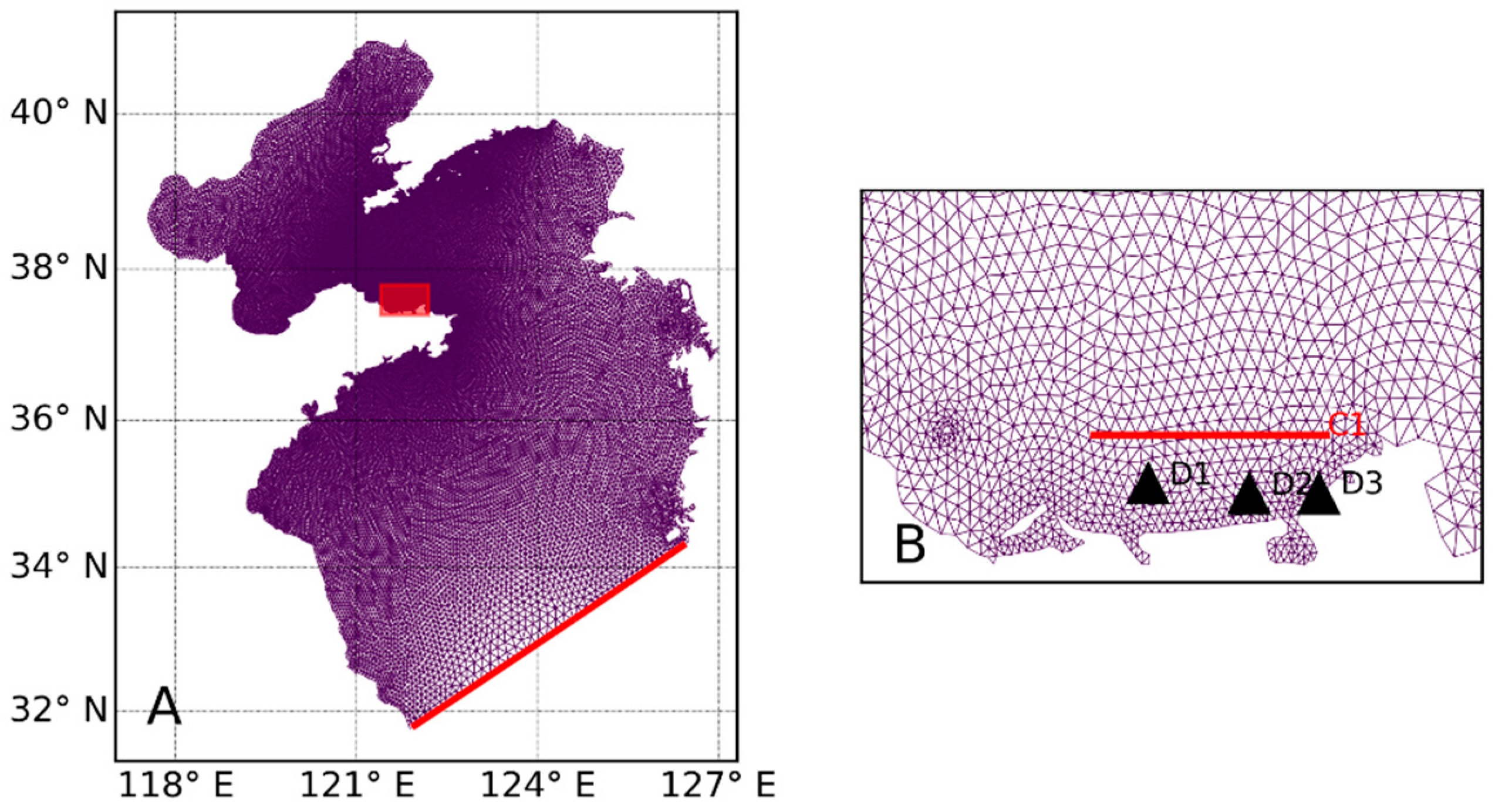
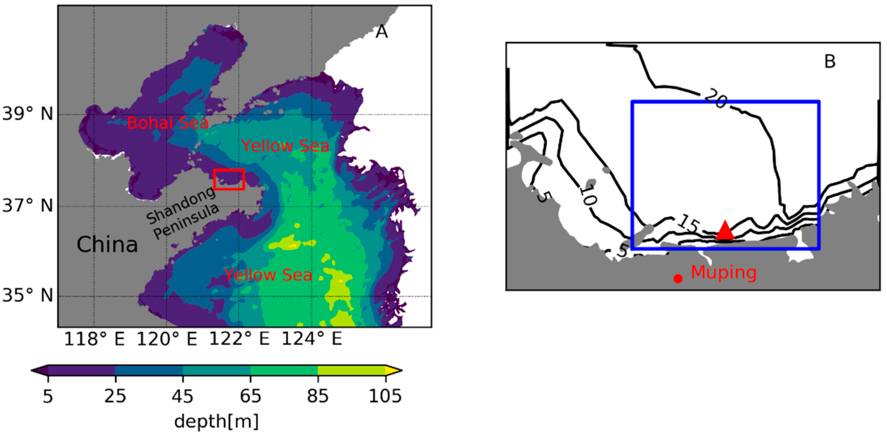
2.1. Study Area

Muping is located in the north coast of Shandong Peninsula. The coastal water of Muping is part of the north Yellow Sea, as shown in Figure 1A. The study area considered herein is limited in the blue frame in Figure 1B, which is about 40 km long (west–east) and 30 km wide (south–north). In most parts of the study area, bottom hypoxia occurs in the summer. The depth of the water in the study area ranges from 5 m to 25 m. The isobath 10 m is only 3 km away from the coastline, while the isobath 20 m is located farther in the west of 121.9° E. A trough exists around 121.9° E, and the isobath 20 m is perpendicular to the coastline in the trough. The depth of the cross-shore axis of the trough reaches up to 23 m. The time zone of the study area is UTC+8. All time-related data or figures are recorded in local time.

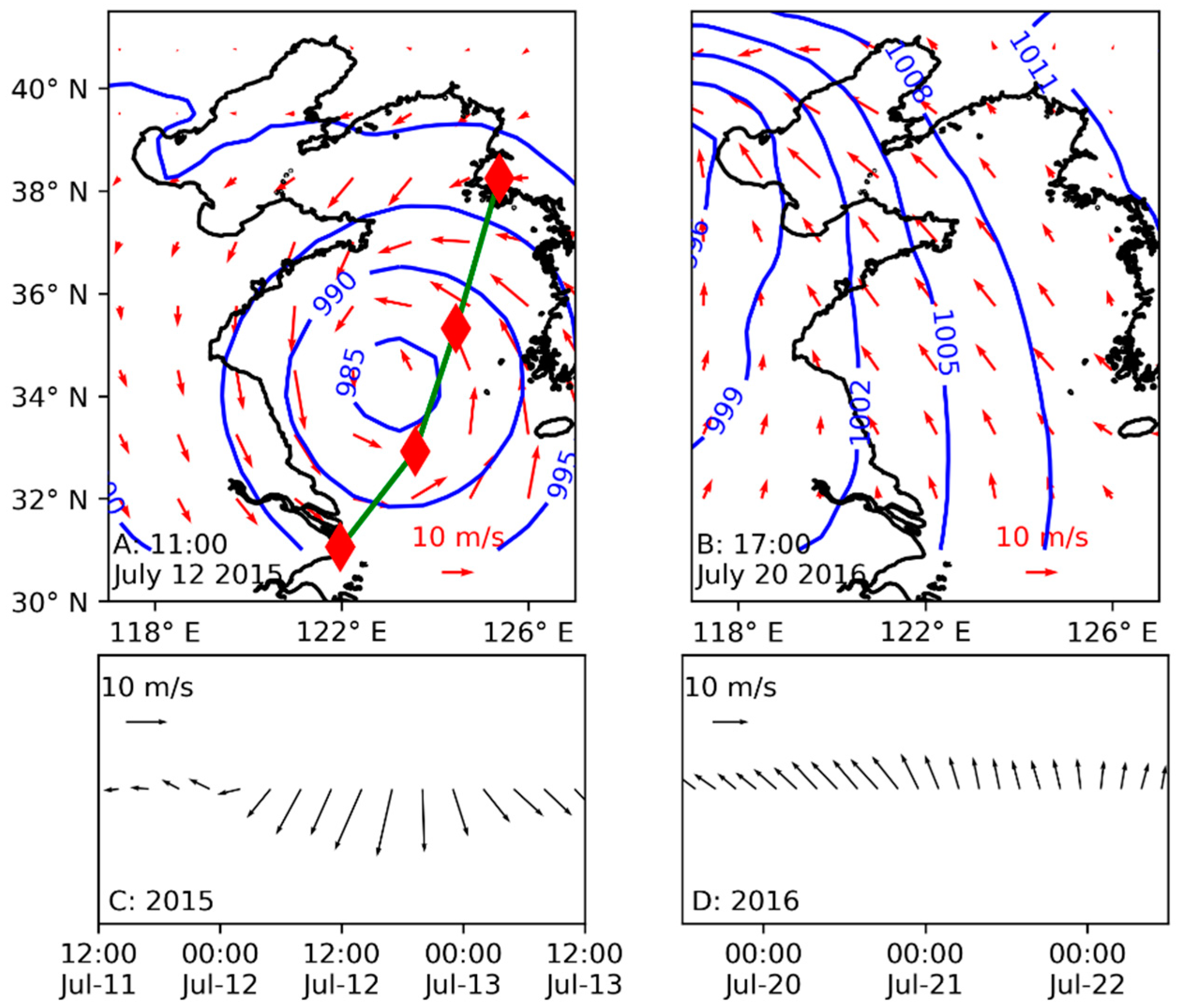
2.2. Two Storm Events

The 2 storm events occurred in July of 2015 and 2016, as shown in Figure 2. They are hereafter called Storm I and Storm II, respectively. Both storms were listed in annual China’s Marine Disaster Bulletin published by the State Ocean Administration of China as the impacted coastal areas suffered significant losses. Storm I was a typhoon named Chan-hom, which was the ninth typhoon in 2015. It originated in the northwest Pacific Ocean. Its intensity grew as it moved toward the northwest. On 12 July, the typhoon center moved northeastward and entered the Yellow Sea. As it approached Muping, the wind speed in the coastal water of Muping increased up to 15.1 m/s at 17:00 on 12 July 2015. The intensity of the typhoon was weaker as it moved northward, and the influence of the typhoon on the coastal water of Muping disappeared at 12:00 on 13 July. The wind direction during Storm I in the coastal water of Muping varied from northeast to northwest (see Figure 2C). The wind direction was almost northerly when the wind speed was maximum. Storm II was induced by an extratropical cyclone system. The low-pressure center was about 1000 km in the southwest of Muping. The dominating wind directions during Storm II were southeast and south. From 00:00 on 20 July 2016 to 05:00 on 22 July 2016, the wind speed in the coastal water of Muping was more than 8 m/s during this storm. The maximum wind speed during Storm II was 11.1 m/s at 20:00 on 20 July 2016.

2.3. Stationary Measurements

In early May 2015, an SBE 21 Thermosalinograph CTD (conductivity, temperature, and depth) sensor was placed on the seabed of site S1 (Figure 1B). The CTD was retrieved in late August of 2015. Timeseries of the bottom sea temperature were measured by the CTD during this period. The same CTD sensor was deployed on the seabed at site S1 again from early July to late August 2016, and the bottom water temperature was measured. At the same time in 2016, a buoy was installed about 200 m in the east of the CTD, measuring the surface temperature during this period. The time interval of all stationary measurements of sea temperature was 10 min.

2.4. Model Configuration

In this paper, a 3-dimension coastal ocean model, Finite Volume Coastal Ocean Model (FVCOM), was used to study the influence of storms on the temperature structure. FVCOM was developed by Chen et al. (2003) [24]. It has the attributes of simple discrete coding, is computationally efficient, and is geometrically flexible. It is very suitable for hydrodynamic modelling of estuarine and coastal regions with a complex irregular coastline and topographical geometry. For detailed descriptions of FVCOM, please refer to the manual (https://wiki.fvcom.pml.ac.uk/; accessed on 26 June 2021). FVCOM has been widely used in ocean modelling studies [25,26,27].

As shown in Figure 3, the model domain covers the whole Yellow Sea and the Bohai Sea. The boundary between the Yellow Sea and East China sea was the open boundary of the model domain. The mesh resolution near the open boundary was set to 15 km and was increased to about 1 km in the study area. The bathymetry data used in the model was extracted from nautical charts. On the open boundary, the hourly water level forecasted by TPXO 7.0 [28] was added. The initial temperature and salinity conditions, as well as the monthly temperature and salinity data on the open boundary, were provided by the Hybrid Coordinate Ocean Model (HYCOM, http://www.hycom.org; accessed on 26 June 2021) [29]. The meteorological data on the sea surface were the ECMWF interim data [30] with a spatial resolution of 0.25° and a time interval of 3 h. The meteorological data included the wind speed, air temperature at 2 m, air pressure, relative humidity, shortwave heat flux, and downward longwave heat flux. The wind stress and the net heat flux were calculated based on the meteorological data.

The model started on 1 January 2013. After a 2-year spin-up period, the model results of 2015 and 2016 were stored for further analysis. In this paper, the model results during the 2 storms were used.

3. Results

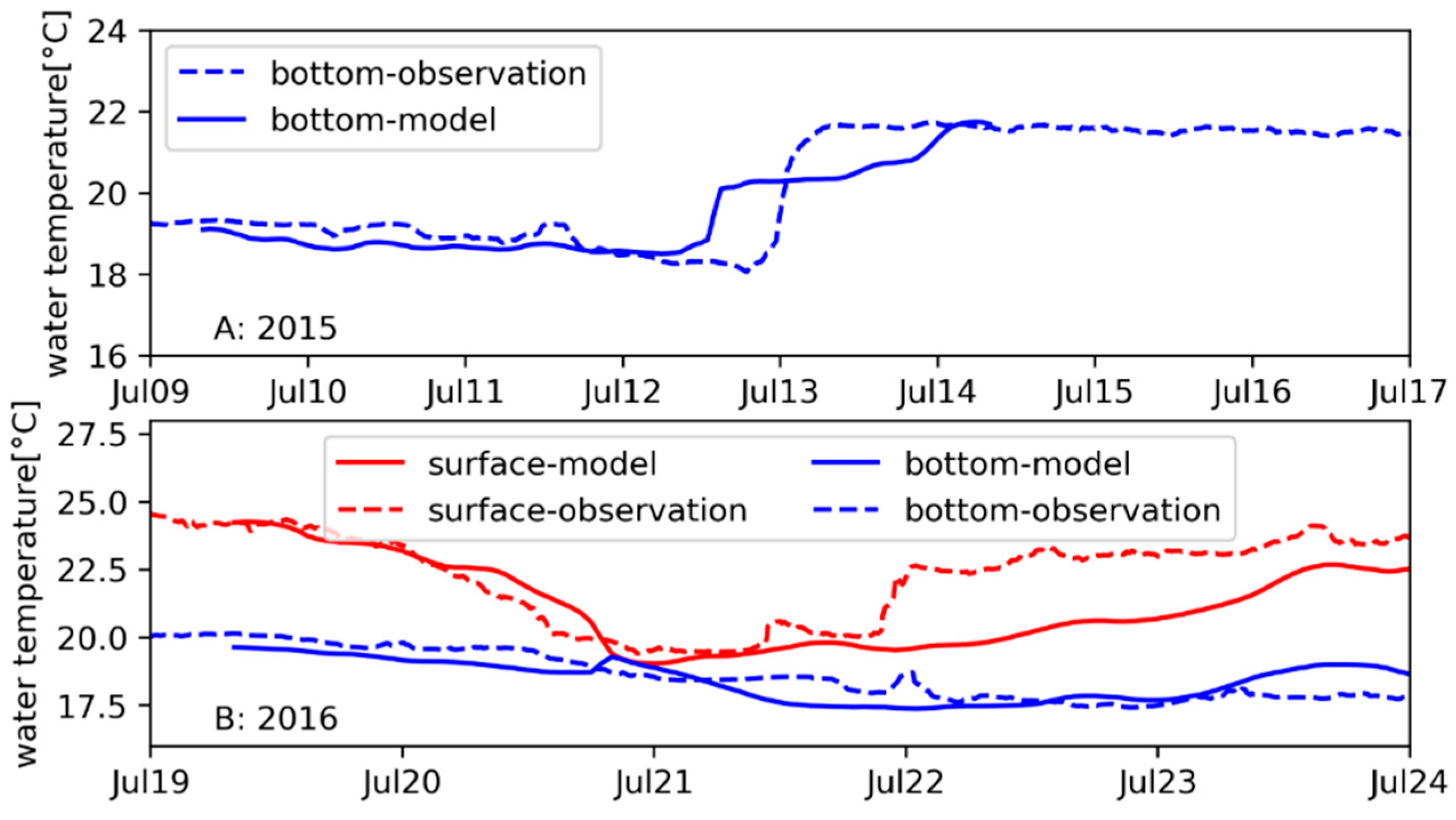
3.1. Model Validation

Figure 4 shows the comparison between the recorded and the modelled temperature data at location S1 during Storm I (Figure 4A) and Storm II (Figure 4B). Since no surface temperature was observed during Storm I, only the bottom temperature was compared. The model simulated the surface and bottom temperature before the two storms relatively well, as the RMSD before the storm was less than 1 °C. During Storm I, the observational data shows that bottom temperature experienced a sharp increase from 18.5 °C to about 22 °C within 7 h. The bottom temperature after the storm was almost the same in the model and the observation, but the time at which the bottom temperature increased significantly occurred in the model 8 h earlier than in the observation. During Storm II, both the surface and bottom temperature decreased when the storm started to impact the study area, as indicated in the observational data. The decreasing rate of surface temperature was greater than the bottom temperature. Consequently, the temperature difference between the surface and the bottom decreased from 4 °C to less than 1 °C after the midday on 20 July. After that, the surface temperature was relatively stable, and the bottom temperature decreased slightly. At 22:00 on 21 July, the surface temperature increased sharply by 2.5 °C within 3 h, while the bottom temperature remained stable. This made the stratification recover to a similar level before Storm II. For the second storm, the model reproduced the decrease in the surface and bottom temperature very well. However, the model overestimated the vertical mixing at the surface, and the bottom temperature was completely mixed at 00:00 on 21 July while this was not the case in the observation.

Overall, the model well simulated the temporal variation of the seawater temperature at the site S1. Furthermore, it captured different evolution patterns of the water temperature during the two storms with different wind directions. Thus, the model results could be used to investigate the influencing mechanism of the wind directions during storms on seawater temperature structure.

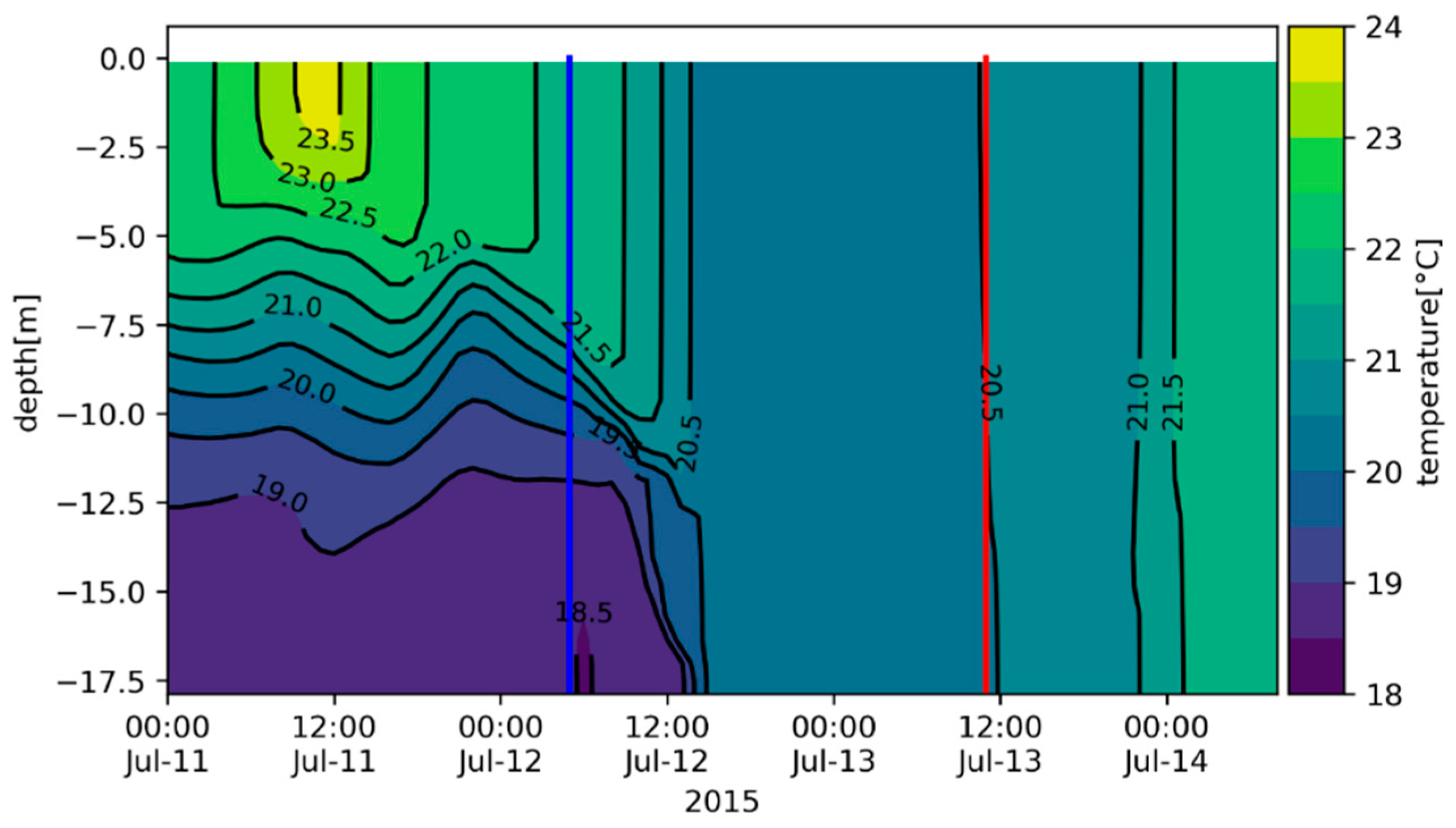
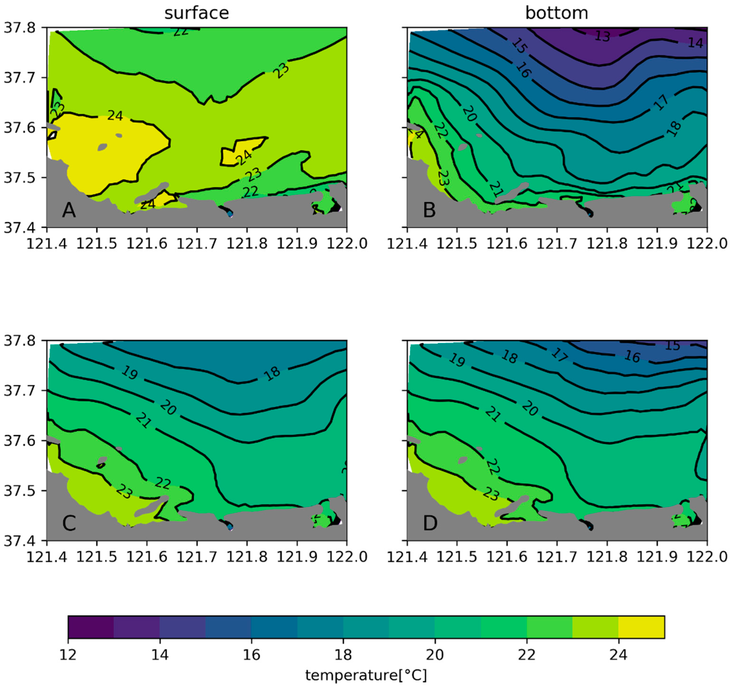
3.2. Responses of Temperature Structure during the Two Storm Events

3.2.1. Temperature Structure Variation during the First Storm

Figure 5 shows the temporal change of temperature over the whole water column at S1 during the first storm. Before the storm (wind speed < 8 m/s), the water column at S1 was well stratified with a temperature difference between surface and bottom exceeding 5 °C. At 05:00 on 12 July 2015, the typhoon storm began to noticeably impact the study area (wind speed > 8 m/s). The surface temperature decreased from 22 °C to 20 °C while the bottom temperature increased by 2 °C within 7 h. At 14:00 on 12 July, the surface temperature and the bottom temperature were almost the same (about 20 °C), which means that the water column became well mixed during the storm. After 11:00 on 13 July, the wind speed decreased and was inferior to 8 m/s. Although the temperature in the whole water column increased within the 2 days following the storm, the water column remained well mixed.

Figure 6 shows the distribution of the surface and bottom temperature before and after the Storm Ⅰ. Before the storm (Figure 6A,B), the surface temperature over the study area was relatively uniform, ranging from 22 °C to 24 °C. The bottom temperature was more variable over space, whereby the bottom temperature nearshore was up to 8 °C higher than offshore at 37.8° N. The storm that occurred at 14:00 on 13 July 2015 caused the surface temperature to decrease by 1–5 °C from nearshore to offshore compare to before the storm, whereas the bottom temperature increased by 1–3 °C. The surface and the bottom temperature were almost the same in the south of isobath 19 °C, indicating that water columns were completely mixed in most of the study area.

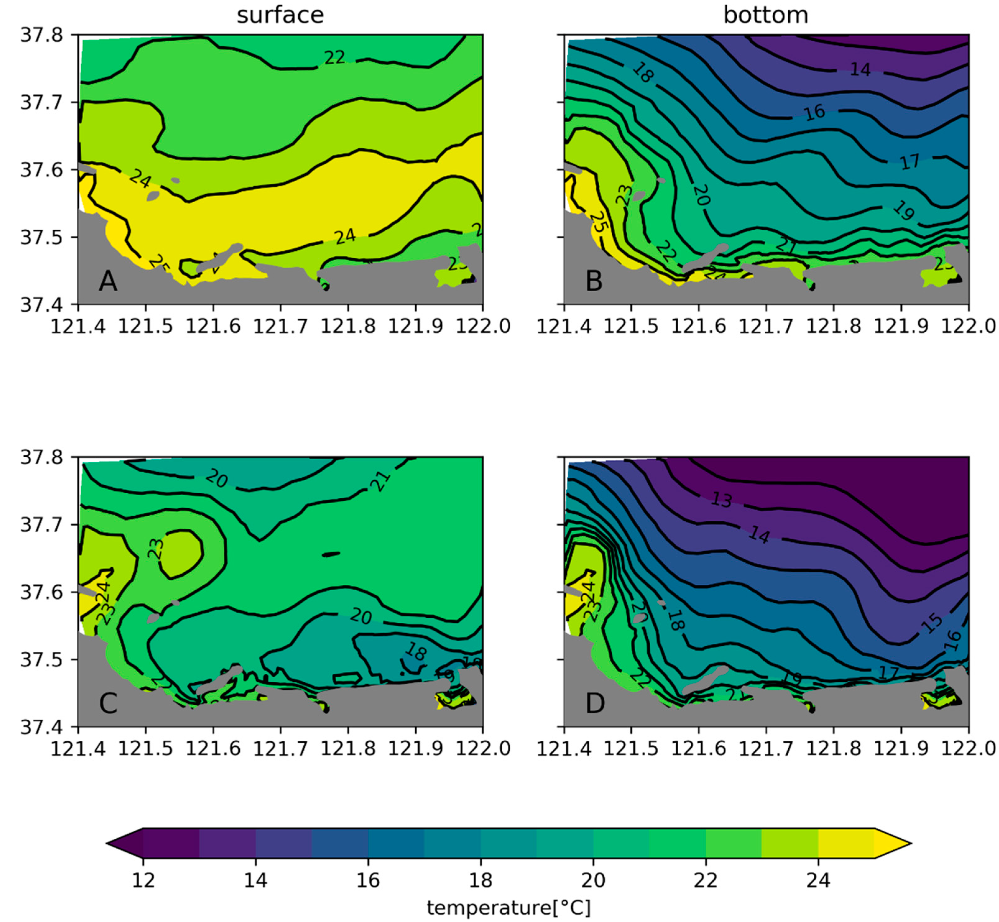
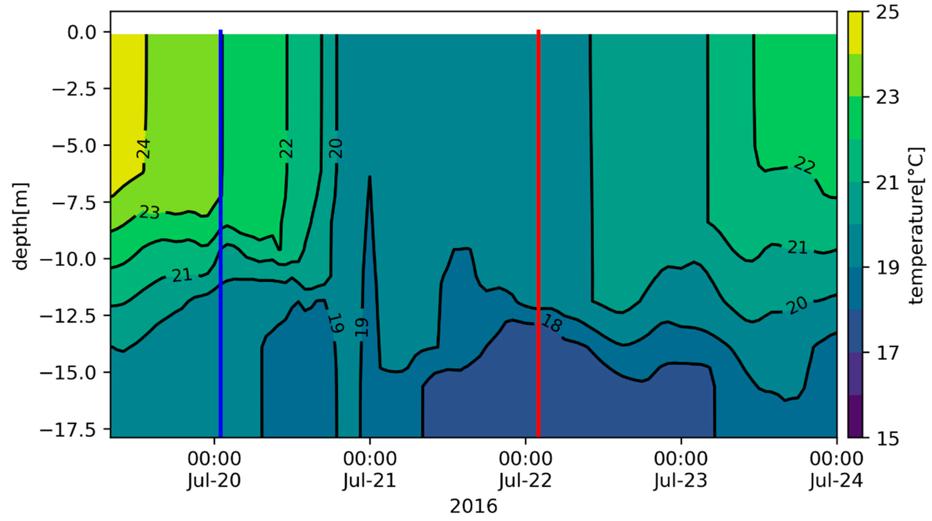
3.2.2. Temperature Structure Variation during the Second Storm

Figure 7 shows the temporal change of the temperature over the whole water column at location S1 during the second storm. Before the storm, the water column was in the state of stratification. The surface temperature was about 24 °C, and the bottom temperature was below 20 °C. Under the influence of strong storm wind, both the surface and bottom temperatures decreased, which did not occur during Storm I, therefore representing a notable difference between the two storm events. From 10:00 to 18:00 on 20 July, the decreasing rate of surface temperature was accelerated, and the depth of the upper mixed layer was increased. At 18:00 on 20 July, the water column was completely mixed with a temperature less than 19 °C, and the bottom temperature continued to decrease to 18 °C. Even if the wind speed was lower than 8 m/s after 02:00 on 22 July, the bottom temperature remained below 18 °C for more than 24 h. However, the temperature in the middle and upper layers increased soon after the storm and water column became stratified once again.

Figure 8 shows the distribution of the surface and bottom temperature before and after the second storm. Before the storm (Figure 8A,B), the surface temperature and the bottom temperature were within the range 22–24.5 °C and 12–23 °C, respectively. During the storm at 00:00 on 22 July, the surface temperature generally decreased by 1–5 °C compared with that before the storm. The surface temperature nearshore experienced a stronger decrease than in the offshore. The lowest surface temperature was less than 18 °C in the southeast corner of the study area, which was at the southern tip of the trough. A cold surface water band could be seen extending from the cold-water center toward the west. Figure 8D shows that all isolines of the bottom temperature moved toward the coastline in comparison with before the storm. For example, the isolines 16–18 °C moved 15–20 km and were very close to the coastline during the storm. The bottom temperature isolines exhibited an abrupt turn to the coastline in the trough area, which fitted well the isobath of the trough.

3.3. Numerical Experiments

3.3.1. Experiments Settings

In summary, during the second storm occurring in July 2016, the temperature showed a different variability pattern than that observed during the first storm. These differences lie in two aspects: (1) During Storm I, the surface temperature decreased and the bottom temperature increased, while during Storm II, both the surface and the bottom water were cooled, and the nearshore surface water experienced a sharper decrease than during Storm I; and (2) Storm I was more effective in breaking down stratification than Storm II.

The maximum wind speed during Storm Ⅰ in the coastal water of Muping was more than 15.0 m/s, which is significantly larger than that recorded in Storm II (11.1 m/s). Hence, it is unclear whether the wind direction was responsible for the temperature structure difference during the two storms. To address this point, a numerical experiment was designed based on the validated model during Storm II (Model_ref). The wind directions (during the storm period) of the other models in the numerical experiment were modified based on the wind data in the reference model. The wind speed magnitude remained the same in all the models in the experiment. The model settings in the experiment are shown in

Table 1. Model settings of the numerical experiment.

Model Run	Descriptions
Model_ref	The well-validated model during Storm II
Model1	South component of the realistic wind → north component
Model2	realistic wind → southerly wind
Model3	realistic wind → northerly wind
Model4	realistic wind → easterly wind
Model5	realistic wind → westerly wind

.

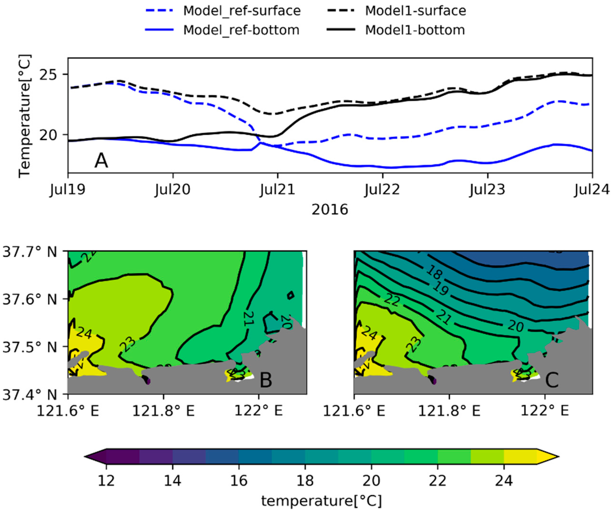
3.3.2. Model_ref vs. Model1

During Storms I and II, the north component of the wind was the dominating component, and the signs of the north component were opposite (Figure 2). It is estimated that the different signs of the north component of wind led to the different patterns of temperature change. Therefore, Model1 was designed to test the response of the temperature to the north component of the wind. Figure 9A shows the timeseries of surface and bottom temperature at S1 simulated by Model_ref and Model1 in the numerical experiment. Unlike in Model_ref, the bottom temperature in Model1 increased and the surface temperature decreased during the storm, which is consistent with the bottom temperature changes observed during Storm I. The surface water cooling was noticeably less significant in Model1, only about 3 °C higher than that in Model_ref. After 22 July, the water column at site S1 in Model1 was almost mixed. Figure 9B,C show the surface and bottom temperature all over the study area at 00:00 on 22 July in Model1. In comparison with the temperature recorded on 19 July before the storm (Figure 8A,B), the surface temperature decreased, while the bottom temperature increased all over the study area in Model1, showing similar patterns to the temperature change in Storm I (Figure 6). This indicates that the temperature variation was sensitive to the north component of the wind and the northward wind component may have influenced the decrease of bottom temperature during Storm II. Stratification was reduced over the study area in Model1 compared with Model_ref. The water columns nearshore became well mixed, but water in the offshore was still more stratified than that during Storm I (Figure 6)). This was obviously due to the stronger wind speed recorded during Storm I.

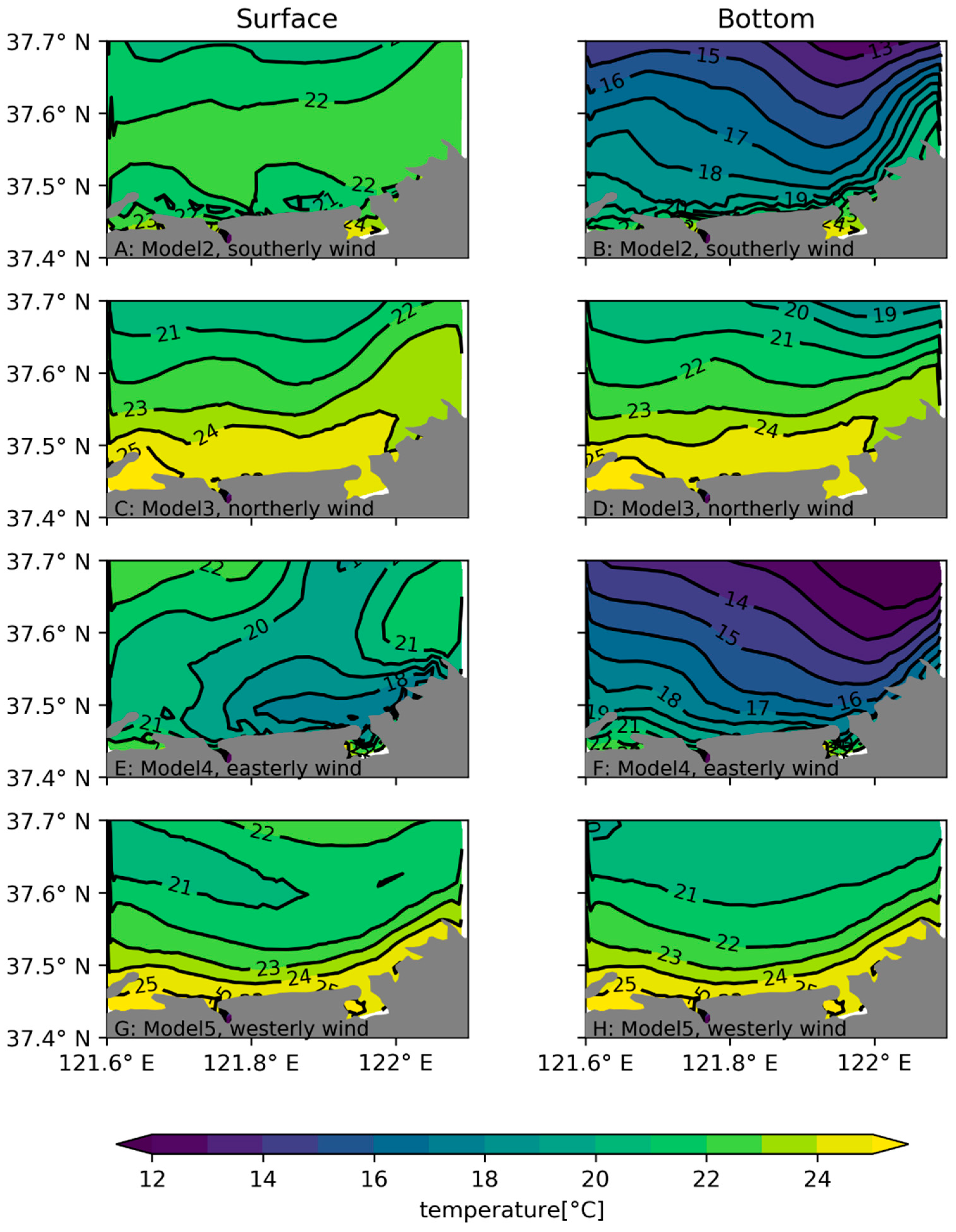
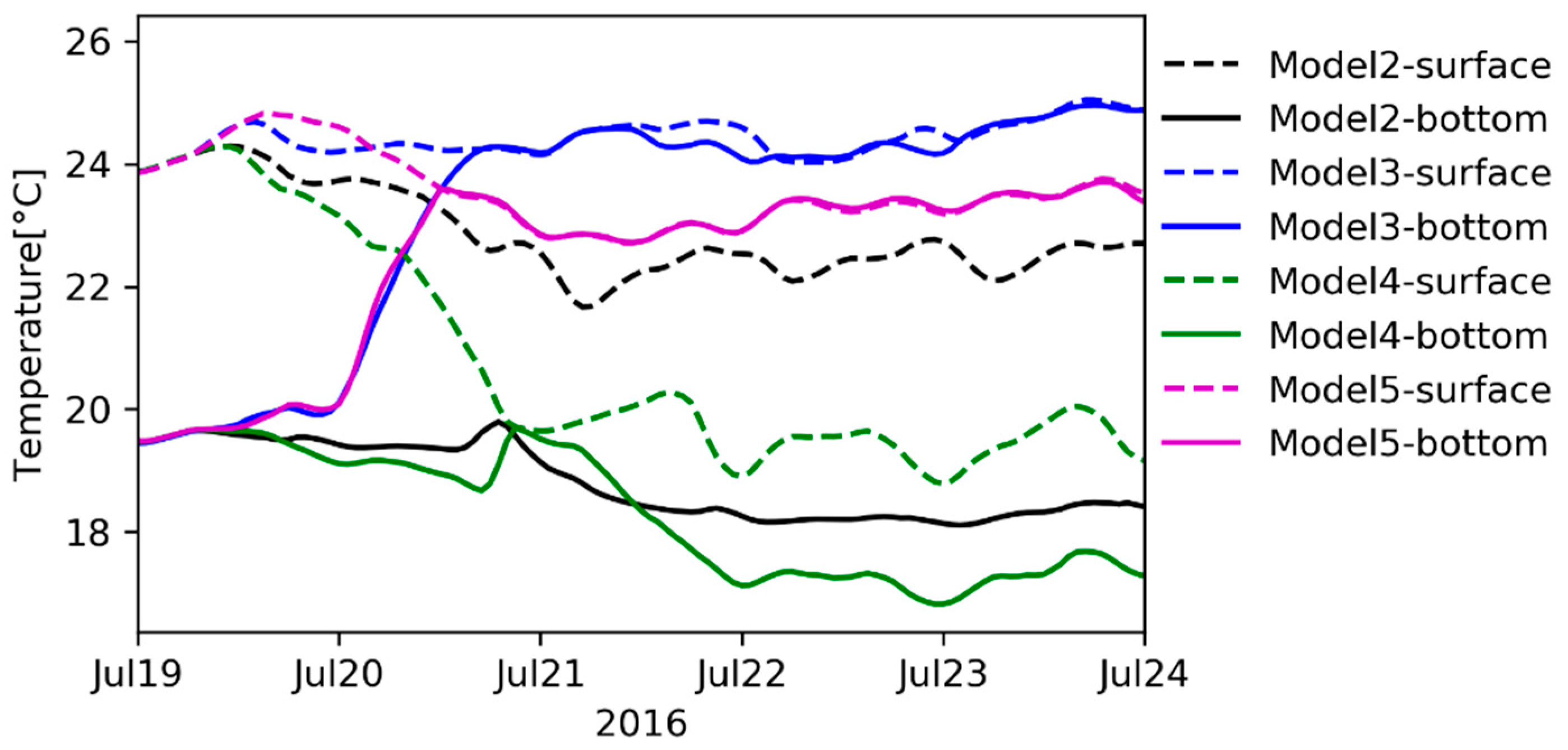
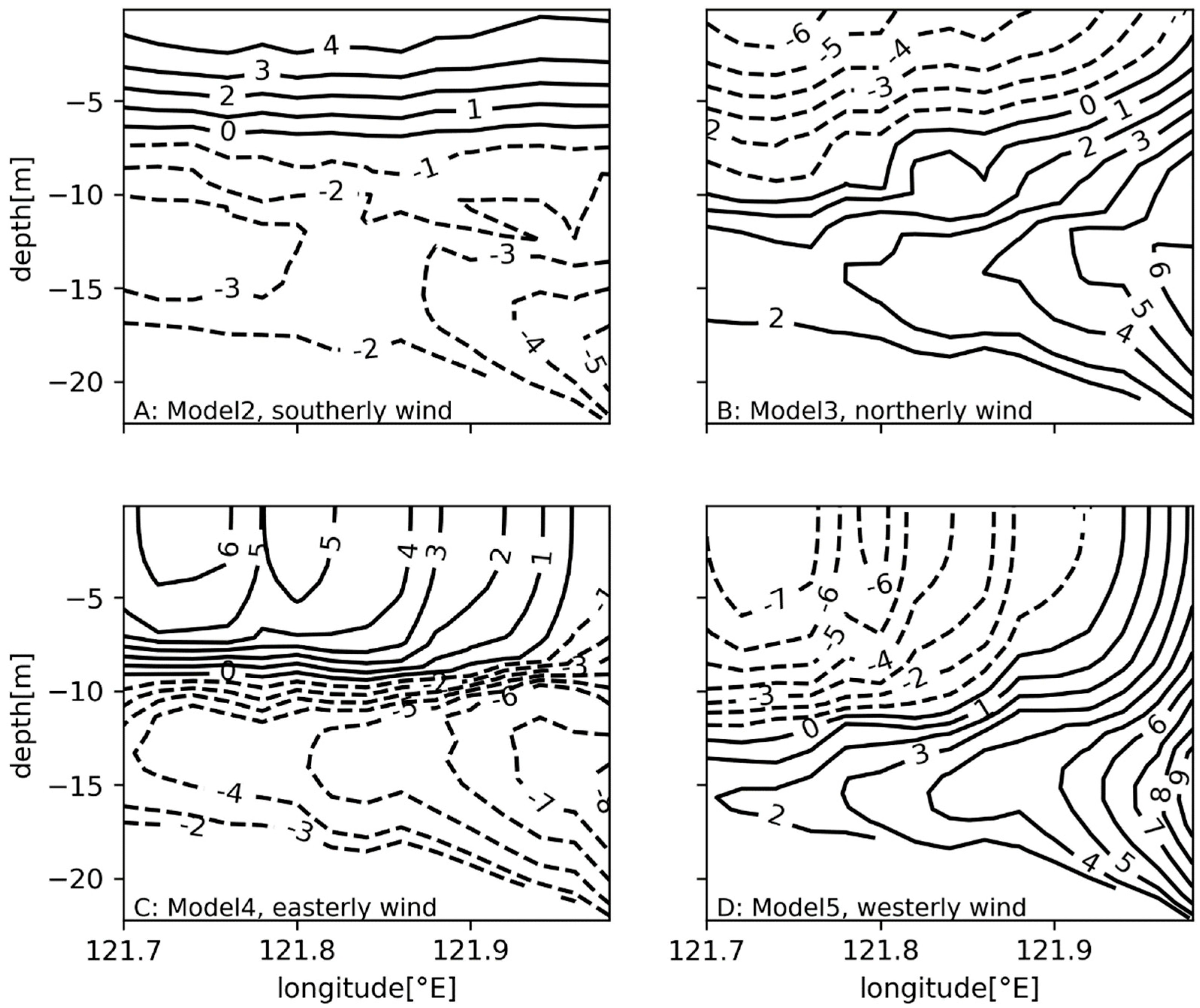
3.3.3. The Response of the Temperature to the Alongshore Wind and Cross-Shore Wind

To gain a better understanding of the response of temperature to the wind directions, the roles of the alongshore and cross-shore winds were investigated. In Model2–5, the wind magnitude remained the same as in Model_ref, and the wind directions were set to south, north, east, and west, respectively. The orientation of the coastline roughly extended west to east. Therefore, the southerly and northerly wind was cross-shore, and the easterly and westerly wind was alongshore.

As shown in Figure 10, the easterly wind and southerly wind had a similar effect on the surface and bottom temperature variation, whereby both the surface and bottom temperature decreased during strong wind at site S1. The bottom temperature under the easterly wind (Model4) at S1 was slightly lower than under the southerly wind (Model2) before 12:00 21 July. After that time, their temperature difference was greater than 1 °C. The surface temperature was about 2 °C lower in Model4. On the other hand, the northerly wind and the westerly wind completely mixed the water column at S1. The surface temperature under northerly wind was about 1 °C higher than under westerly wind.

Figure 11 shows the snapshots of the surface and bottom temperature at 00:00 on 22 July simulated by Model2–5. In Model2 and Model4, the bottom temperature decreased all over the study area at 00:00 on 22 July compared with that observed at 19:00 on 19 July (Figure 8), while the bottom temperature increased in Model3 and Model5. However, the isolines during the easterly windstorm were located closer to the coastline than during the northerly wind storm. This indicates that the easterly wind brought more cold water from the deeper sea to the study area. The surface temperature in Model4 was also colder than in Model2 and similar to the cold-water band along 37.5° N in the Model_ref (Figure 8C), and there was also a cold-water band at the same location in Model4. However, this cold-water band did not appear in Model2, which implies that the cold-water band was related to the easterly wind component in Model_ref. Under the influence of the northerly wind and westerly wind, the surface temperature and the bottom temperature were almost the same. The surface temperature was about 1 °C higher than the bottom temperature only at 37.7° N near the northmost boundary of the study area. Although water columns were well mixed in the two models, the water in Model3 was generally warmer than in Model5 at 00:00 on 22 July.

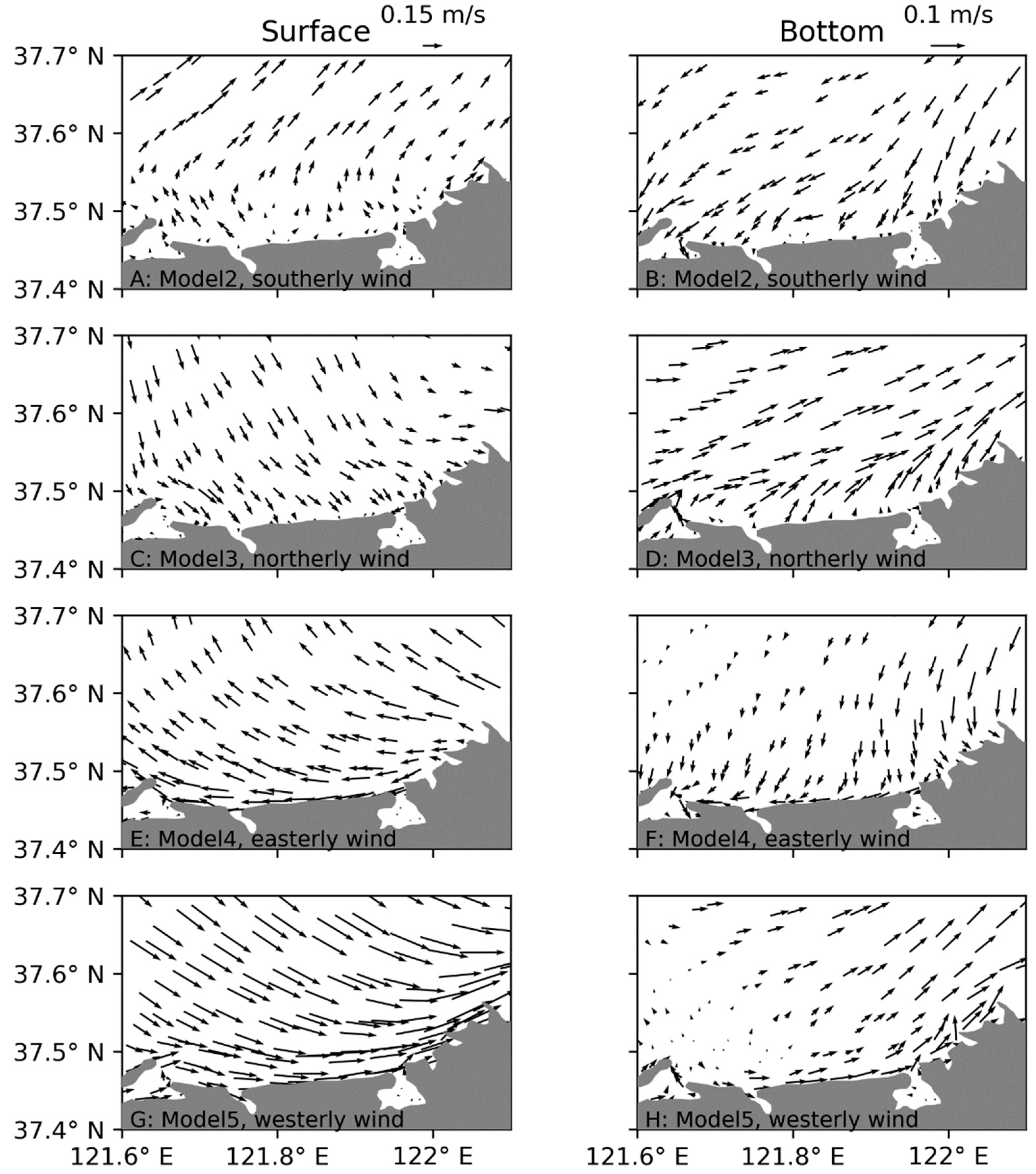
3.3.4. Current Velocity Induced by Alongshore and Cross-Shore Wind

The notable difference between the two storms was the intrusion of cold water from offshore during Storm II, which implies that cross-shore transport may have been significantly enhanced during the second storm. The current velocity and the cross-shore discharge were also investigated. The hourly current velocity in Model2–5 was averaged over the period from 00:00 on 20 July to 01:00 on 21 July 2016. The time-averaged current velocity excluded tidal component and kept the wind-induced current. The surface and bottom time-averaged currents in Model2–5 are shown in Figure 12. The surface current in the four models is generally consistent with the surface Ekman velocity theory. The surface current directions were approximately 45° to the right of the wind directions in most parts of the study area. Near the coastline, the surface current directions were almost parallel to the coastline. The cross-shore components of surface current pointed toward the north in Model2 and Model4 and toward the south in Model3 and Model5. The southerly wind and the easterly wind produced a shoreward bottom current, while in the other two Models, the bottom current was overall directed toward the northeast. The orientation of the coastline in the study area was almost west–east. The easterly wind was upwelling-favorable, and the westerly wind was downwelling-favorable according to the generally accepted viewpoint on the wind-upwelling system. From the surface and bottom current velocities in Figure 12, one can infer that the southerly wind was upwelling-favorable and the northerly wind was downwelling-favorable. A strong bottom temperature gradient existed before the storm, whereby the bottom temperature decreased rapidly from nearshore to offshore (Figure 6B). During the upwelling-favorable wind, the bottom current transported colder water toward nearshore. The bottom cooling due to the intruding cold-water had a greater impact than the warming rate due to vertical mixing, which resulted in the continuous decrease of the temperature at S1, as shown in Figure 10. The decrease in the bottom temperature helped stabilize the water column and reduced vertical turbulent mixing. On the other hand, under the influence of downwelling-favorable wind, the bottom current transported warmer water toward the offshore and the surface current transported colder water to the nearshore. Both the surface and the bottom transport had a positive effect on vertical mixing. Therefore, it was easier to reduce stratification during the downwelling-favorable wind.

As shown in Figure 2, the wind direction in Storm I ranged from the northeast to northwest. The north component of the wind was always southward and significantly larger than the east component. Therefore, the wind during Storm I was downwelling-favorable, while the wind during Storm II was upwelling-favorable. The different patterns of temperature structure during Storm I and II could be well explained by the above analysis.

As cross-shore transport play a critical role in temperature structure variation, cross-shore discharge over 20 July through a transect C1 (see Figure 3B) was investigated. The transect is on 37.55° N and extends from 121.7° E to 122.0° E. The discharge per unit area (m³) is defined as ${{\displaystyle \int }}_{t_1}^{t_2}vdt$, where $t_1$ is 00:00 on 20 July, t2 is 00:00 on 21 July, and $v$ is the cross-shore component (north component) of the current velocity on a certain layer. The depth-variable discharge per unit area through the transect C1 in Model2–5 is presented in Figure 13. During the upwelling-favorable wind in Model2 and Model4, water flowed northward in the upper layers and southward in the lower layers. The wind-induced Ekman surface current was right of the wind direction. The subsurface current then rotated clockwise and was smaller than the surface current. Thus, the cross-shore component of the current velocity decreased rapidly with depth during the southerly wind. During the easterly wind, the current velocity also decreased with depth, but its direction was from northwest to north with depth. The cross-shore component may not have decreased as rapidly as during northerly wind. Therefore, the thickness of the outflow layer was smaller in Model2 (southerly wind) than in Model4 (easterly wind) (Figure 13A,C). The easterly wind transported more upper-layer water toward the north than northerly wind ($<2\times {10}^5$ m³), which resulted in a stronger discharge ($2~4\times {10}^5$ m³) in the lower layers. This explains why the bottom temperature was lower during the easterly wind than during the southerly wind (Figure 11). Both the northerly wind and westerly wind produced upper-inflow and lower-outflow discharge patterns, but the upper-layer discharge in Model5 (westerly wind) was larger than in Model3 (northerly wind). The offshore surface water was colder than the nearshore surface water. Therefore, more surface cold water flowed southward and caused the surface temperature to lower, as shown in Figure 11.

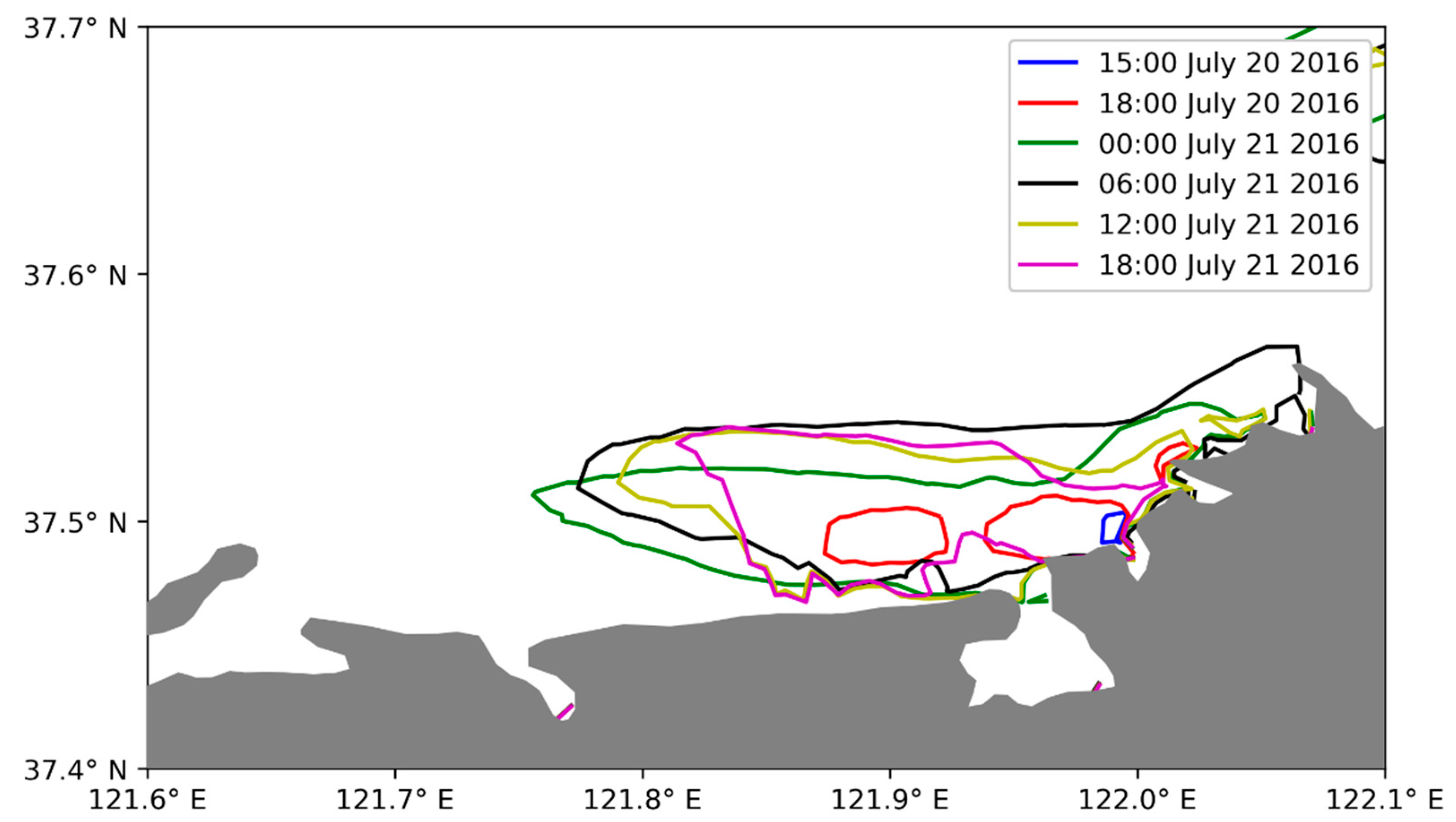
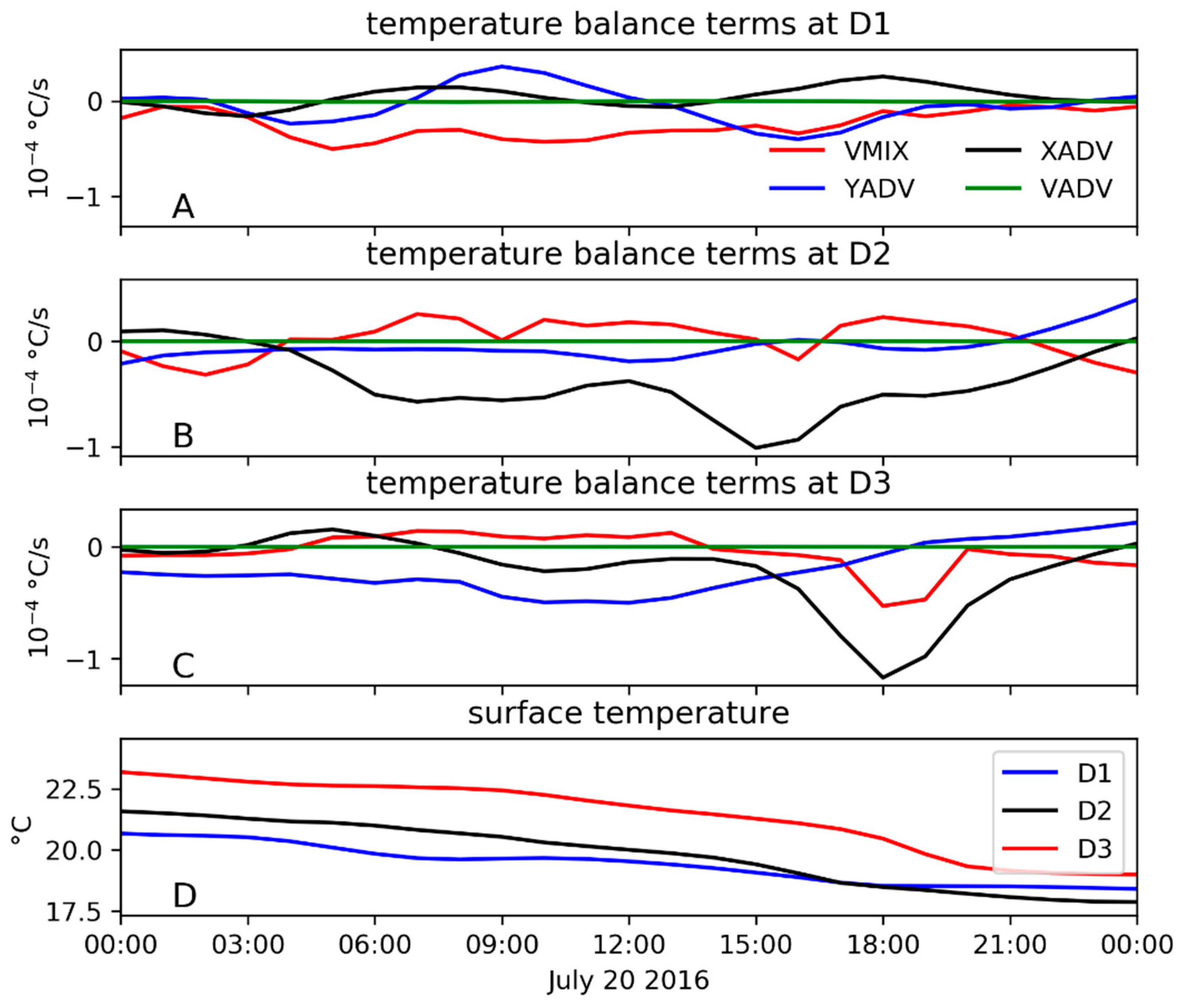
3.4. The Formation Mechanism of a Surface Cold-Water Band

Figure 8 shows that a cold-water band formed during Storm II at around 37.5° N and extended to about 20 km from west to east. Site S1 was inside the west part of the cold-water band. The substantial surface water cooling and reduced stratification at S1 are attributed to the surface cold-water band. As the minimum surface temperature during Storm II was about 19 °C, the isolines 19 °C of surface temperature at different times are presented in Figure 14. The surface temperature of 19 °C did not appear until at 15:00 on 20 July. At that time, surface water at temperatures lower than 19 °C was limited in a small nearshore area around 122.9° E (enclosed by the blue isoline), where the depth was smaller than 8 m. At 18:00 on 20 July, the cold-water zone (lower than 19 °C) was expanded toward the west. A westward cold-water tongue extended from 121.75° N to 122.05° N at 00:00 on 21 July. After that, the cold-water tongue receded and moved a short distance northward. In the numerical experiment, the easterly wind generated the westward surface current over the cold-water band, while the southerly wind-generated northward surface current (Figure 12). Accordingly, in Model4 with the easterly wind, there was also a cold-water band (Figure 11) as in Model_ref (Figure 8), but no cold-water band appeared in Model2 with the southerly wind. This implies that the westward component of wind during Storm II played an important role in the formation of the cold-water band.

A temperature balance analysis was performed using the FVCOM model output to explain the formation of the cold-water band quantitatively. The temperature equation is written as

$$\frac{\partial T}{\partial t}=\left(-\frac{\partial \left(uT\right)}{\partial x}\right)+\left(-\frac{\partial \left(vT\right)}{\partial y}\right)+\left(-\frac{\partial \left(wT\right)}{\partial z}\right)+\frac{\partial }{\partial z}\left(K_h\frac{\partial T}{\partial z}\right)$$

(1)

where $T$ is the water temperature; $t$ is the time; $u$, $v$, and $w$ are the east, the north, and the vertical component of current velocity, respectively; and $K_h$ is the turbulent eddy viscosity. The left-hand-side term in Equation (1) represents the local temporal temperature change. Local temperature change is caused by the four terms on the right-hand side. These are the east component of the horizontal advection (XADV), the north component of horizontal advection (YADV), the vertical advection (VADV), and the vertical mixing (VMIX). Along with the cold-water band, three sites D1, D2, and D3 were specified for the surface temperature balance analysis (see Figure 3B). The water depth at the sites was 6.5 m, 14.1 m, and 18.0 m at D1, D2, and D3, respectively. Site D1 was located where the cold water was originally formed. D3 was at the same location as S1, where the instrument was deployed. D2 was between D1 and D3 on the cold-water band. During the whole day of 20 July, the surface temperature decreased at all the three sites (Figure 15D). At D1, the vertical mixing dominated the surface cooling. At D2, surface cooling was mainly caused by vertical mixing in the first 2 h. Then, XADV became the primary process causing the reduction of surface water temperature throughout the remainder of 20 July. The surface cooling was so strong that the surface water was even colder than its adjacent lower layer temperature as VMIX was positive. At D3, YADV was the dominant process of the surface cooling before 15:00 on 20 July. After that, the surface cooling was mainly driven by XADV. Figure 15 shows that the cooling mechanism at D1 was different from D2 and D3. The depth at D1 was only 6.5 m. The strong wind and tidal current could mix the surface and lower-layer cold water. The surface cold water at D1 was subsequently transported toward the west. The cold surface water from D1 arrived at D2 earlier than D3, which explains why the minimum XADV at D2 was earlier than at D3. VADV was very small compared with the vertical mixing and the horizontal advection at all the three sites, although the wind in Storm Ⅱ was upwelling-favorable.

4. Discussions and Summaries

This study investigated the effect of two summer storm events with opposite wind directions on water temperature structures in the coastal water of Muping, China. A well-validated numerical ocean model FVCOM was used for this study.

Most of the time in the summer, a strong temperature gradient exists in the offshore bottom water of Muping. The patterns of the water temperature variation during the two storms were different. Wind during the Storm I was downwelling-favorable, which means that the bottom current was toward offshore. Wind during the Storm II was upwelling-favorable, and the induced bottom current was shoreward. During Storm I, the surface temperature decreased and the bottom temperature increased. The temperature of the water columns over the study area became almost mixed. However, during the second windstorm, both the surface and bottom temperature in the study area decreased.

The downwelling-favorable wind was more effective at eroding stratification than the upwelling-favorable wind. During the downwelling-favorable wind, the shoreward surface current transported colder water from offshore, and the nearshore warmer bottom water was transported to the direction of offshore. Therefore, the horizontal advection of the heat during the downwelling-favorable wind weakened the stratification. On the other hand, during the upwelling-favorable wind, the effect of the bottom intruding cold water was greater than the vertical wind mixing, causing continuous bottom water cooling in the study area. The bottom cold water made the water column more stable and suppressed mixing. These results are consistent with the findings reported when hurricanes attacked the east coast of the United States [21,31].

In the study area, the coastline extended from west to east. It is generally regarded that upwelling-favorable or downwelling-favorable wind is parallel to the coastline [32]. Few previous studies have recognized that the cross-shore wind is upwelling-favorable or downwelling-favorable. The numerical experiment in this paper indicates that the cross-shore wind could also be upwelling-favorable (southerly) or downwelling-favorable (northerly) as it could also produce cross-shore transport with opposite directions in the upper and lower layers. This may be valid in shallow coastal waters and under the influence of strong wind. Strong cross-shore wind transported significantly more surface water than moderate wind along the cross-shore direction. Then, the lower-layer water had to be transported to the opposite direction due to the mass balance. However, under the easterly wind, both the upper-layer and lower-layer transport were larger than the southerly wind. More bottom deeper cold water intruded nearshore, making the surface and bottom water colder than during the southerly wind. During a storm, the northerly wind is also as downwelling-favorable as the westerly wind. Due to stronger surface transport, surface water was colder during the westerly wind than during the northerly wind. Apart from in the study area investigated herein, a cross-shore wind of moderate magnitude can also be upwelling-favorable, such as in small-scale bays (2 × 3 km) [33] and narrow bays (5 × 40 km) [34]. Therefore, whether cross-shore wind can be upwelling-favorable or downwelling-favorable depends on wind speed magnitude, the coastal water size, and the coastline shape.

Although wind during Storm II was upwelling-favorable, the effect of upwelling to cool surface water was minor. As the wind is very strong during a storm, vertical mixing is the primary process for cooling surface water other than upwelling. Apart from wind mixing, large wind can also generate a strong alongshore surface current which redistributes surface temperature. A distinct feature was the appearance of a cold-water band during Storm II. Longshore cold-water bands are common in upwelling-influenced coastal waters [35,36,37]. The positions of cold-water bands depend on the wind magnitude [38] and topography [37,39]. Unlike classic upwelling-related cold-water bands, the cold-water band observed herein was formed due to the vertical mixing and westward surface advection. Although the southerly wind was also upwelling-favorable, such surface cold-water band did not appear under the southerly wind.

Strong summer stratification in the study area slows down the vertical diffusion of DO from upper layers to lower layers and may sometimes lead to hypoxia. Storms are important to relieve DO deficiency. Storms are rare and short in summer, but strong winds may significantly alter the stratification process in shallow coastal waters as shown in this paper. The wind direction during storms was found to play an important role in sea temperature variation. Under normal weather conditions, the dominant wind direction was south or southwest in the study area. The wind speed was weak but lasted for a longer time than the storms. Future research will be conducted to explore the influence of wind direction under normal weather conditions on temperature structures and stratification and their effects on annual variation of sea temperature.

References

1. Yang, B.; Gao, X.; Xing, Q. Geochemistry of organic carbon in surface sediments of a summer hypoxic region in the coastal waters of northern Shandong Peninsula. Cont. Shelf Res. 2018, 171, 113–125. [Google Scholar] [CrossRef]
2. Du, J.; Shen, J. Decoupling the influence of biological and physical processes on the dissolved oxygen in the Chesapeake Bay. J. Geophys. Res. Ocean. 2015, 120, 78–93. [Google Scholar] [CrossRef] [Green Version]
3. Zhu, J.; Zhu, Z.; Lin, J.; Wu, H.; Zhang, J. Distribution of hypoxia and pycnocline off the Changjiang Estuary, China. J. Mar. Syst. 2016, 154, 28–40. [Google Scholar] [CrossRef]
4. Zhu, J.; Shi, J.; Guo, X.; Gao, H.; Yao, X. Air-sea heat flux control on the Yellow Sea cold water mass intensity and implications for its prediction. Cont. Shelf Res. 2018, 152, 14–26. [Google Scholar] [CrossRef]
5. Lee, S.-H.; Beardsley, R.C. Influence of stratification on residual tidal currents in the Yellow Sea. J. Geophys. Res. Ocean. 1999, 104, 15679–15701. [Google Scholar] [CrossRef] [Green Version]
6. Wei, H.; Yuan, C.; Lu, Y.; Zhang, Z.; Luo, X. Forcing mechanisms of heat content variations in the Yellow Sea. J. Geophys. Res. Ocean. 2013, 118, 4504–4513. [Google Scholar] [CrossRef]
7. Li, J.; Li, G.; Xu, J.; Dong, P.; Qiao, L.; Liu, S.; Sun, P.; Fan, Z. Seasonal evolution of the Yellow Sea cold water mass and its interactions with ambient hydrodynamic system. J. Geophys. Res. Ocean. 2016, 121, 6779–6792. [Google Scholar] [CrossRef] [Green Version]
8. Li, X.; Sun, X.Y.; Zhang, Q.F.; Niu, F.X.; Yao, Z.G. Seasonal evolution of the Northern Yellow Sea cold water mass. Mar. Sci. Bull. 2013, 15, 16–25. [Google Scholar]
9. Zhang, S.W.; Wang, Q.Y.; Lü, Y.; Cui, H.; Yuan, Y.L. Observation of the seasonal evolution of the Yellow Sea cold water mass in 1996–1998. Cont. Shelf Res. 2008, 28, 442–457. [Google Scholar] [CrossRef]
10. Yang, H.-W.; Cho, Y.-K.; Seo, G.-H.; You, S.H.; Seo, J.-W. Interannual variation of the southern limit in the Yellow Sea bottom cold water and its causes. J. Mar. Syst. 2014, 139, 119–127. [Google Scholar] [CrossRef]
11. Lee, J.-h.; Pang, I.-C.; Moon, J.-H. Contribution of the Yellow Sea bottom cold water to the abnormal cooling of sea surface temperature in the summer of 2011. J. Geophys. Res. Ocean. 2016, 121, 3777–3789. [Google Scholar] [CrossRef]
12. Wu, X.; Wang, H.; Bi, N.; Song, Z.; Zang, Z.; Kineke, G.C. Bio-physical changes in the coastal ocean triggered by typhoon: A case of Typhoon Meari in summer 2011. Estuar. Coast. Shelf Sci. 2016, 183, 413–421. [Google Scholar] [CrossRef]
13. Ni, X.; Huang, D.; Zeng, D.; Zhang, T.; Li, H.; Chen, J. The impact of wind mixing on the variation of bottom dissolved oxygen off the Changjiang Estuary during summer. J. Mar. Syst. 2016, 154, 122–130. [Google Scholar] [CrossRef] [Green Version]
14. Ma, Z.; Han, G.; de Young, B. Modelling the response of Placentia Bay to hurricanes Igor and Leslie. Ocean. Model. 2017, 112, 112–124. [Google Scholar] [CrossRef]
15. Scully, M.E.; Friedrichs, C.; Brubaker, J. Control of estuarine stratification and mixing by wind-induced straining of the estuarine density field. Estuaries 2005, 28, 321–326. [Google Scholar] [CrossRef]
16. Xie, X.; Li, M. Effects of wind straining on estuarine stratification: A combined observational and modeling study. J. Geophys. Res. Ocean. 2018, 123, 2363–2380. [Google Scholar] [CrossRef]
17. Chereskin, T.K.; Price, J.F. Upper Ocean Structure: Ekman Transport and Pumping. In Encyclopedia of Ocean Sciences, 3rd ed.; Cochran, J.K., Bokuniewicz, H., Yager, P., Eds.; Oxford University Press: Oxford, UK, 2019; pp. 80–85. [Google Scholar]
18. Scully, M.E. Physical controls on hypoxia in Chesapeake Bay: A numerical modeling study. J. Geophys. Res. Ocean. 2013, 118, 1239–1256. [Google Scholar] [CrossRef] [Green Version]
19. Lentz, S.; Shearman, K.; Anderson, S.; Plueddemann, A.; Edson, J. Evolution of stratification over the New England shelf during the Coastal Mixing and Optics study, August 1996–June 1997. J. Geophys. Res. Ocean. 2003, 108, 8–14. [Google Scholar] [CrossRef]
20. Guan, S.; Zhao, W.; Huthnance, J.; Tian, J.; Wang, J. Observed upper ocean response to typhoon Megi (2010) in the Northern South China Sea. J. Geophys. Res. Ocean. 2014, 119, 3134–3157. [Google Scholar] [CrossRef] [Green Version]
21. Forsyth, J.; Gawarkiewicz, G.; Andres, M.; Chen, K. The interannual variability of the breakdown of fall stratification on the new jersey shelf. J. Geophys. Res. Ocean. 2018, 123, 6503–6520. [Google Scholar] [CrossRef]
22. Weinke, A.D.; Biddanda, B.A. Influence of episodic wind events on thermal stratification and bottom water hypoxia in a Great Lakes estuary. J. Great Lakes Res. 2019, 45, 1103–1112. [Google Scholar] [CrossRef]
23. Survey, E.B.o.C.B. (Ed.) Survey of China Bays; China Ocean Press: Beijing, China, 1991; Volume 3. [Google Scholar]
24. Chen, C.; Beardsley, R.C.; Franks, P.J.S.; Keuren, J.V. Influence of diurnal heating on stratification and residual circulation of Georges Bank. J. Geophys. Res. Ocean. 2003, 108. [Google Scholar] [CrossRef]
25. Cazenave, P.W.; Torres, R.; Allen, J.I. Unstructured grid modelling of offshore wind farm impacts on seasonally stratified shelf seas. Prog. Oceanogr. 2016, 145, 25–41. [Google Scholar] [CrossRef] [Green Version]
26. Jiang, L.; Xia, M. Modeling investigation of the nutrient and phytoplankton variability in the Chesapeake Bay outflow plume. Prog. Oceanogr. 2018, 162, 290–302. [Google Scholar] [CrossRef]
27. Wu, X.-G.; Tang, H.-S. Coupling of CFD model and FVCOM to predict small-scale coastal flows. J. Hydrodyn. Ser. B 2010, 22, 284–289. [Google Scholar] [CrossRef]
28. Egbert, G.D.; Erofeeva, S.Y. Efficient inverse modeling of barotropic ocean tides. J. Atmos. Ocean. Technol. 2002, 19, 183–204. [Google Scholar] [CrossRef] [Green Version]
29. Halliwell, G.R. Evaluation of vertical coordinate and vertical mixing algorithms in the HYbrid-Coordinate Ocean Model (HYCOM). Ocean. Model. 2004, 7, 285–322. [Google Scholar] [CrossRef]
30. Dee, D.P.; Uppala, S.M.; Simmons, A.J.; Berrisford, P.; Poli, P.; Kobayashi, S.; Andrae, U.; Balmaseda, M.A.; Balsamo, G.; Bauer, P.; et al. The ERA-Interim reanalysis: Configuration and performance of the data assimilation system. J. R. Meteorol. Soc. 2011, 137, 553–597. [Google Scholar] [CrossRef]
31. Miles, T.; Seroka, G.; Glenn, S. Coastal ocean circulation during Hurricane Sandy. J. Geophys. Res. Ocean. 2017, 122, 7095–7114. [Google Scholar] [CrossRef]
32. Hu, J.; Wang, X.H. Progress on upwelling studies in the China seas. Rev. Geophys. 2016, 54, 653–673. [Google Scholar] [CrossRef]
33. Walter, R.K.; Reid, E.C.; Davis, K.A.; Armenta, K.J.; Merhoff, K.; Nidzieko, N.J. Local diurnal wind-driven variability and upwelling in a small coastal embayment. J. Geophys. Res. Ocean. 2017, 122, 955–972. [Google Scholar] [CrossRef]
34. Cheng, P.; Valle-Levinson, A.; Winant, C.D.; Ponte, A.L.S.; de Velasco, G.G.; Winters, K.B. Upwelling-enhanced seasonal stratification in a semiarid bay. Cont. Shelf Res. 2010, 30, 1241–1249. [Google Scholar] [CrossRef]
35. Montoya-Sánchez, R.A.; Devis-Morales, A.; Bernal, G.; Poveda, G. Seasonal and intraseasonal variability of active and quiescent upwelling events in the Guajira system, southern Caribbean Sea. Cont. Shelf Res. 2018, 171, 97–112. [Google Scholar] [CrossRef]
36. Ruiz-Castillo, E.; Gomez-Valdes, J.; Sheinbaum, J.; Rioja-Nieto, R. Wind-driven coastal upwelling and westward circulation in the Yucatan shelf. Cont. Shelf Res. 2016, 118, 63–76. [Google Scholar] [CrossRef]
37. Su, J.; Pohlmann, T. Wind and topography influence on an upwelling system at the eastern Hainan coast. J. Geophys. Res. Ocean. 2009, 114. [Google Scholar] [CrossRef] [Green Version]
38. Chen, Z.; Yan, X.-H.; Jiang, Y.; Jiang, L. Roles of shelf slope and wind on upwelling: A case study off east and west coasts of the US. Ocean. Model. 2013, 69, 136–145. [Google Scholar] [CrossRef]
39. Howatt, T.M.; Allen, S.E. Impact of the continental shelf slope on upwelling through submarine canyons. J. Geophys. Res. Ocean. 2013, 118, 5814–5828. [Google Scholar] [CrossRef]
Figure 1. (A) The location of the study area is in the red frame. (B) The study area is indicated in the blue rectangular frame. The black isolines are isobaths (m) in the study area and adjacent waters; the red triangular is the location of a stationary measurement (S1).
Jmse 09 00710 g001
Figure 2. Air pressure and wind speed (10 m) of the two storm events. (A) Air pressure (hPa, blue isolines) and wind field (red vectors) over the Yellow Sea and the Bohai Sea at 11:00 12 July 2015 (Storm I). The green line indicates the track of Typhoon Chan-hom; 4 red diamonds are the locations of typhoon centers at 00:00, 08:00, 15:00 on 12 July 2015, and 02:00 on 13 July 2015 from south to north. (B) Air pressure (blue isolines) and wind field (red vectors) over Yellow Sea and Bohai Sea at 17:00 on 20 July 2016 (Storm II). (C) Timeseries of wind vectors at site S1 during Storm Ⅰ. (D) Timeseries of wind vectors at S1 during Storm II. Wind speed (10 m) and air pressure data are ECMWF interim data.
Jmse 09 00710 g002
Figure 3. (A) The whole model mesh of FVCOM. The red line indicates the open boundary. (B) The zoom-in model mesh surrounding the study area. The red horizontal line indicates a transection C1 used for analysis in Section 3.3. The 3 black triangles D1, D2, and D3 are used for temperature balance analysis in Section 3.4.
Jmse 09 00710 g003
Figure 4. Comparisons of temperature between model results and observational data during Storm I (A) and Storm II (B).
Jmse 09 00710 g004
Figure 5. Time-depth diagram of the modelled temperature at location S1 during Storm I. The blue and red lines indicate the start and end time of Storm I, respectively (wind speed > 8 m/s).
Jmse 09 00710 g005
Figure 6. Spatial distribution of the surface (A,C) and bottom (B,D) temperature before (12:00 on 11 July 2015 (A,B)) and during (14:00 on 13 July 2015 (C,D)) Storm I.
Jmse 09 00710 g006
Figure 7. Time-depth diagram of modelled temperature at location S1 during Storm II. The blue and red line indicate the start and end time of Storm I (wind speed > 8 m/s).
Jmse 09 00710 g007
Figure 8. Spatial distribution of surface (A,C) and bottom (B,D) temperature before (12:00 on 19 July 2016 (A,B)) and during (00:00 on 21 July 2016 (C,D)) Storm II.
Jmse 09 00710 g008
Figure 9. (A) Timeseries of temperature simulated by Model_ref and Model1. (B) Spatial distribution of surface temperature simulated by Model1 at 00:00 on 22 July 2016. (C) Spatial distribution of bottom temperature simulated by Model1 at 00:00 on 22 July 2016.
Jmse 09 00710 g009
Figure 10. Timeseries of surface and bottom temperature simulated by Model2–5.
Jmse 09 00710 g010
Figure 11. Distribution of surface (A,C,E,G) and bottom (B,D,F,H) temperature simulated by Model2–5.
Jmse 09 00710 g011
Figure 12. Surface and bottom time-averaged current velocities in Model2–5. Surface and bottom current velocities simulated by the Model2 are displayed in (A,B) respectively. Surface and bottom current velocities simulated by the Model3 are displayed in (C,D) respectively. Surface and bottom current velocities simulated by the Model4 are displayed in (E,F) respectively. Surface and bottom current velocities simulated by the Model5 are displayed in (G,H) respectively.
Jmse 09 00710 g012
Figure 13. Discharge (m3) per unit area across the section C1 over 20 July 2016 in Model2 (A), Model3 (B), Model4 (C), and Model5 (D). The sign of inflow (toward the coast) was negative (dashed lines), and outflow was positive (solid lines). For better display, the isoline values are 10 5 times of discharge.
Jmse 09 00710 g013
Figure 14. Isolines 19 °C of surface temperature at different times during Storm II.
Jmse 09 00710 g014
Figure 15. Surface temperature balance terms during 20 July 2016 at D1 (A), D2 (B), and D3 (C). (AC) share the same legend as (A). (D) Surface temperature at D1, D2, and D3 during 20 July 2016.
Jmse 09 00710 g015