Article

Process-Based Model Prediction of Coastal Dune Erosion through Parametric Calibration

1
Department of Convergence Study on the Ocean Science and Technology, Korea Maritime & Ocean University, Busan 49112, Korea
2
Department of Ocean Engineering, Korea Maritime & Ocean University, Busan 49112, Korea
3
Department of Marine Science and Convergence Engineering, Hanyang University, Ansan 15588, Korea
4
School of Civil and Construction Engineering, Oregon State University, Corvallis, OR 97331-2302, USA
*
Authors to whom correspondence should be addressed.
J. Mar. Sci. Eng. 2021, 9(6), 635; https://doi.org/10.3390/jmse9060635
Submission received: 31 March 2021 / Revised: 31 May 2021 / Accepted: 2 June 2021 / Published: 7 June 2021
(This article belongs to the Special Issue The Coastal Response Modeling)

Abstract

:
Coastal dunes are important morphological features for both ecosystems and coastal hazard mitigation. Because understanding and predicting dune erosion phenomena is very important, various numerical models have been developed to improve the accuracy. In the present study, a process-based model (XBeachX) was tested and calibrated to improve the accuracy of the simulation of dune erosion from a storm event by adjusting the coefficients in the model and comparing it with the large-scale experimental data. The breaker slope coefficient was calibrated to predict cross-shore wave transformation more accurately. To improve the prediction of the dune erosion profile, the coefficients related to skewness and asymmetry were adjusted. Moreover, the bermslope coefficient was calibrated to improve the simulation performance of the bermslope near the dune face. Model performance was assessed based on the model-data comparisons. The calibrated XBeachX successfully predicted wave transformation and dune erosion phenomena. In addition, the results obtained from other two similar experiments on dune erosion with the same calibrated set matched well with the observed wave and profile data. However, the prediction of underwater sand bar evolution remains a challenge.

1. Introduction

Coastal areas are attractive to humans due to opportunities for tourism, trade, transportation, fishing, and so forth. However, these areas are subjected to storm-induced flooding and erosion, which are threats to coastal safety in the coastal region. Indeed, the coastal dune acts as the natural defense line against the impact of storm flooding and rising sea level as well as providing natural habitats to local flora and fauna [1]. In general, berm and dune systems are eroded by winter storms, resulting in relatively steep beach profiles and sand bars; whereas in the summer, the eroded sand piles up once again and results in a mild beach profile [2]. Recent extreme storm events, such as Hurricanes Katrina and Sandy, have destroyed the dune and berm systems along the coasts of Texas and New Jersey, resulting in severe flood damage to the hinterland [3,4]. Therefore, a reliable predictive model for the storm-driven dune erosion is consistently required to assess coastal management strategies against external force by rising sea levels and the possibility of more intense storms. Unfortunately, the hydrodynamic and morphological response to storms in the coastal area is highly complex due to the combination of sediment motions (soil dilatancy and grain stabilization, etc.) and wave nonlinearity effects (wave breaking, skewness, and asymmetry). Therefore, there have been various numerical studies to predict the storm-driven dune evolution process in terms of field measurements [5,6,7] and physical experiments [8,9,10]. Over the past decades, semi-empirical, parametrized numerical models such as SBeach [11] and CSHORE [12] have been developed to assess storm-induced erosion and overwash of coastal dunes under extreme conditions. Although the existing tools predict bar behavior on scales of months to years, they are limited to estimate storm-induced dune erosion, overwash, and breaching of coastal dunes. Therefore, considerable efforts have been made to improve the model accuracy around the waterline resulting in the development of a new process-based and time-dependent 2DH model called XBeach [13]. This model is an open-source and off-the-shelf model, which solves coupled equations for predicting wave propagation, sediment transport, and bed level change in the nearshore. The low-frequency wave motion plays an essential role in the incident band swash and morphological change on dissipative sandy beaches during extreme conditions [14]. The XBeach model can assess the storm-induced erosion of coastal areas to coastal erosion induced by extreme storm surges and is widely used to evaluate the performance of existing and future coastal protection projects. Although the XBeach model can predict the morphodynamics on storm impact of the beach/dune system regarding the long wave motions, the model results with default settings substantially overestimate the beach/dune erosion [9,14] and are unable to correctly model the sand bar formation [9].
Numerous studies have extended and validated the XBeach model to improve the model capability for predicting the morphodynamic storm impact of beach/dune systems. To overcome the overestimation of the cross-shore sediment transport and erosion volume, McCall et al. [6] suggested applying artificial limiters for maximum sediment concentration and critical Shields parameter in the XBeach model. However, these sediment transport limiters are not physically based and have led to even worse prediction of dune breaching in some cases [15]. Therefore, as an alternative approach, the bed slope effect on the incipient motion as well as the concept of hindered erosion by soil dilatancy was implemented to improve model performances for dune erosion and breaching events [15]. Both the bed slope and dilatancy effect achieved an acceptable agreement with experiment data, while the wave shape parameter yielded much better results with field data. The XBeach model uses a wave-action equation based on a phased-averaged approach for short waves and hence does not account for the wave shape. Waves approaching the shoreline transform from sinusoidal to skewed in the shoaling zone and then obtain a highly asymmetric shape in the wave breaking zone [16]. The wave skewness and asymmetry affect the sediment suspension and transport, and ultimately beach morphology evolution. As reported by Van Geer et al. [17], nine empirical parameters (i.e., fw, cf, gamma, gammax, beta, alpha, wetslp, facSk, and facAs) in XBeach called WTI (Wettelijk Toets Instrumentarium) settings were optimized for the Dutch Coast using the database of 1D flume experiments and 2DH field cases, in the framework project WTI2017, to enhance XBeach simulation results for dune safety assessment in the Netherlands. Despite various works on calibrations to improve model prediction, the implementation of the bed slope effect, wave shape, and other calibration factors in XBeach cannot completely solve the overestimation of berm/dune erosion volumes. Hence, many studies still attempt to improve the model performance continuously. For instance, the latest release of the XBeach model (version 1.23.5527, XBeachX release) includes the new physical formation for the bermslope effect [18,19] that focuses on swash zone profile changes and TMA (Texel, Marsen, and Arsloe) spectrum [20] for wave boundary forcing. The former is a practical approach to reduce significant erosion induced by complex processes in the limited swash zone and the latter is a JONSWAP (Joint North Sea Wave Project) spectrum [21] with the shallow water effect.
The present study aims to test and calibrate a process-based model (XBeachX) to improve the simulation accuracy of dune erosion from a storm event. For that objective, this study recalibrates the breaker slope (beta) and wave shape parameters (facSk and facAs) in WTI settings, and applies bermslope transport under TMA wave boundary forcing. The results were compared using the dataset of large-scale physical models conducted in the large wave flume of the Hinsdale Wave Research Laboratory at Oregon State University [22]. Model prediction of the wave height and the bed level change were assessed based on the model-data comparisons, and the calibrated XBeachX successfully reproduced the wave transformation and dune erosion phenomena.

2. Method

2.1. Experimental Setup

Two-dimensional large-scale movable experiments were conducted to investigate the morphodynamics in a sandy dune beach in the Large Wave Flume at the Hinsdale Wave Research Laboratory at Oregon State University by [22]. The flume dimension was 104 m × 3.7 m × 4.6 m (length × width × depth). Oregon beach sands with a median diameter of 0.22 mm were used to reproduce a sandy dune beach in the flume. The initial profile of dune and beach was selected based on the various east coast and Gulf coast dune survey results in the United States. The dune and beach were built in the flume at a 1:6 geometric scale.
The storm wave conditions were selected based on the field observation during a nor’easter storm that eroded dune profiles along Assateague Island, Virginia, U.S. As shown in Table 1, eight different random waves with different water levels, wave heights, and wave periods were generated to reproduce the entire storm event by using the TMA spectrum including pre-storm, great erosion event (SC3 and SC4), and post-storm [9,10]. Eight resistance-type wave gages and three ultrasonic wave gauges were installed to measure the water surface elevations from the deeper region to the shallower region. Acoustic sensors, MTA (Multi Transducer Array), and a laser range finder were used to survey the profile below and above the water level, respectively. More detailed information for the experimental setup can be found in [9,10]. Figure 1 shows the experimental setup of this study. The coastal dune was initially set up and was eroded, and an underwater sand bar was formed after the wave generation.

2.2. Numerical Setup

Numerical simulation was carried out using XBeach, which is widely used to predict waves, currents, sediment transport, and morphology change under various wave conditions in both 1D and 2D. Many researchers have validated the model in a large number of cases for not only hydrodynamics [23,24,25] but also morphological changes [6,14,19,26]. This model provides three modes for hydrodynamics: the stationary mode, surfbeat mode, and non-hydrostatic mode. The stationary mode solves the wave-averaged equation, and therefore infragravity motions are neglected. The surfbeat mode calculates the short-wave variation on the wave group and the long waves that are associated with them, separately. The non-hydrostatic mode allows the propagation and decay of individual waves. After hydrodynamic processes, XBeach simulates sediment transport and bed level change based on the determined time step and boundary conditions. The stationary mode is generally selected when relatively small or when short wave motions are simulated [27] and neglects infragravity waves, which is vital for prediction of the dune and beach erosion during the storm condition. The non-hydrostatic mode has required more computational cost due to higher resolutions of the numerical grid and has not yet been tested and validated extensively with sediment transport formulations in the model. This study uses the surfbeat mode and the latest XBeachX version, which includes new physical formulation (e.g., bermslope transport) and a new boundary condition (i.e., TMA spectrum) rather than the older version, which only used the JONSWAP spectrum. In this study, the XBeach modeling was conducted under the TMA wave boundary condition with a peak enhanced factor, γ = 3.3, because the above-mentioned laboratory experiment was also set by the same condition.
Grid, bathymetry, and sand properties such as D50 (median diameter) and porosity are based on large wave-flume data, as described in Section 2.1. These input data are exactly the same as the previous study [9], as shown in Table 2. The grid size of a model domain has various resolutions from 0.15 m at the dune area to 2 m offshore under the appropriate CFL (Courant-Friedrichs-Lewy) criterion to compute stably with maximum performance and reduction of computational time. Water levels are set up consistently with Table 1, and wave heights for spectral boundary conditions are defined using wave heights observed by the closest wave gauge to a wave maker.
Many semi-empirical parameters are defined in the XBeach model and set as default values. As previously mentioned, these default values tend to overestimate dune erosion and show poor model performance. For example, the previous study [9] showed that the default settings considerably overestimated the bed level changes and sediment transport and thus the dune was totally breached in the end. To solve the problem, WTI settings were developed, which improved the numerical model performance, but the results in the previous study with WTI settings [9] indicated overestimation near the swash zone. Therefore, the present study suggests the need for re-calibration of wave shape parameters and breaker slope coefficients among WTI settings and investigation of the bermslope transport under wave boundary forcing (TMA).

2.3. Calibration Procedure

In the previous study, XBeach simulations successfully reproduced the infragravity wave runup in the above-mentioned experiment data through the calibration of wave and sediment transport parameters [10]. However, the result was obtained through time-dependent tuning of wave and sediment transport parameters, which limited the application in other cases. On the other hand, this study adopts a sequential calibration procedure to improve a model performance that predicts dune erosion and the resulting bed level changes across the surf and swash zone. The process consists of three stages of calibration. Each step is linked to a breaker slope parameter, wave asymmetry and skewness, and a bermslope parameter, respectively. The flow chart for the procedure is presented in Figure 2. First of all, either the wave dissipation factor or the breaker slope parameter can be calibrated in the case of under- or over-estimation of wave conditions across the surf zone. Further explanation of those two parameters is discussed in the following section. Secondly, two user-defined wave shape parameters that consider skewed and asymmetric transformation when the waves propagate in the shoaling and surf zone are used for calibration of the morphodynamic process. Thirdly, the user-defined bermslope coefficient can be considered to resolve an unrealistic bermslope of the simulated results, as reported by the previous study [9]. Wave shape parameters affect onshore sediment transport in large part of profiles across the shoaling, surf, and swash zone. On the contrary, the bermslope transport term affects limited areas near the waterline (see Section 3.3 for details on the bermslope term). Therefore, this study calibrates wave shape parameters first to improve overall profile prediction and then solves the overestimation problem of the swash zone by adjusting bermslope parameters, which is similar to previous studies [19,25,28].

3. Results

3.1. Wave Calibration

Wave dissipation in the nearshore is caused by the bed friction, breaking, and surface roller. WTI settings and several studies use wave dissipation (alpha, α) [25,29], which is related to breaking, and the breaker slope coefficient (beta, β) [29], which is related to the surface roller, as calibration factors. The Xbeach model calculates the effect of wave surface roller using Equation (1) [27] with those two coefficients, contributing to the shoreward kinetic energy and resulting in radiation stresses and wave-induced forces so that they would affect the prediction of wave height and runup in the surf and swash zone. However, the wave dissipation factor ( α ) did not contribute to significant improvement of the underestimation of wave height in the swash zone in the present study (not presented here), resulting in larger RMSE than the result from a breaker slope factor (β). Therefore, the alternative wave calibration factor, beta (β), is adopted to solve the limitation, as mentioned above. The roller energy balance (Equation (1)) that contains kinetic energy can be calculated by the following equation of x, y, and θ   space:
E r t + E r cos θ x + E r csin θ y = D w D r D w = 2 α Q b E w T r e p ,   Q b = 1     exp ( H r m s / H m a x   n ) D r = 2 g β E r c
where E r is the roller energy, D w and D r are the dissipations by breaking and surface rollers, energy of wave is E w , fraction of breaking waves is Q b , representative wave period is T r e p , root-mean square and maximum wave height are H r m s and H m a x , wave celerity is c, and gravity acceleration is g.
In the present study, wave calibration (WCB) was carried out before the morphodynamic calibration presented in Figure 2 by estimating Root Mean Square Error (RMSE). Varying breaker slope coefficients were used to hindcast accurate wave height, comparing them with the measured ones. Subsequently, optimal values were adopted using the trial and error calibration method. Figure 3 illustrates the results of significant wave heights (Hs) after beta calibrations. Each panel shows the transformation of Hs from offshore to the dune after storm conditions (SC3, upper panel, and SC4, lower panel, respectively). The breaker slope factor does not influence the offshore wave heights before wave breaking because the roller energy balance is applied in the surf zone, but with more influence during the severe condition (i.e., SC4) compared with milder conditions (before SC4). As a result, a reduced breaker slope factor (beta = 0.085), which denotes less dissipation due to the surface roller, improves the prediction of wave transformation in both the surf and swash zone (solid red line in Figure 3). Consequently, optimized wave calibration input obtained by beta is used here to evaluate the suitability of wave shape and bermslope transport to predict accurate morphological change.

3.2. WTI Settings Calibration

XBeach model contains numerous semi-empirical parameters to predict the morphodynamic process [6,13], and model results with default parameters substantially overestimate the beach/dune erosion. As reported by van Geer et al. [17], the nine semi-empirical parameters in XBeach showed a big influence on the model result and are called the WTI settings. In particular, the wave skewness (facSk) and asymmetry (facAs) make considerable contributions to the sediment transport and beach morphology evolution [5,30], because wave skewness and asymmetry are closely related to wave non-linearity and onshore sediment transport. They are also connected to the migration of nearshore bars [28,31]. Hence, only two calibration parameters among the nine in WTI settings are determined. In this study, fifteen different values of the two parameters (No. (1–15) in Table 3) are simulated to optimize TMA results with the calculation of each BSS (Brier-Skill-Score [32]).
BSS = 1 [ z b , c z b , m z b , m 2 / z b , o z b , m 2 ]
Index z b , o, c, and m denote bed level, initial, computed, and measured, respectively, and z b , m indicates the error of the measured bed level that is neglected in this study. Each value range of BSS is categorized as 1.0–0.8 (Excellent), 0.8–0.6 (Good), 0.6–0.3 (Reasonable/fair), 0.3–0 (Poor), and <0 (Bad) [32].
No.2–No.7 in Table 3 is simulated to identify the sensitivity between facAs and facSk. In Figure 4, varying facAs with facSk = 0.13 (No.2–No.4, upper panel) and varying facSk with facAs = 0.13 (No.5–No.7, lower panel) show different volume changes with time. Erosion (positive) above MSL occurs during the entire simulation (18 h) under simulations No.2–No.7. Higher values for the two factors produce less excessive erosions compared with the measured profile based on volume changes. The volume change of No.7 (facSk = 0.38) is 5.42 m 2 while the measured result is 4.32 m 2 . However, the volume change of No. 4 (facAs = 0.38), the opposite value of No.7, is 4.39 m 2 , which shows good agreement with the measured profile. This finding shows that facAs appears to be more sensitive when facSk varies with the same magnitude.
Figure 5 shows good agreement with relatively intense storm conditions (SC4) compared with milder conditions (SC3). Note that BSS for the rest of the scenario (SC1, SC2, and SC5–SC7) is omitted for brevity. Case 1 (blue circle) and Case 2 (red circle) indicate bed level above 0 m and between −2 and 0 m, respectively. In contrast with the excellent prediction (Maximum BSS = 0.989) for Case1, Case2 for SC4 presented lower values (BSS = 0.799) than Case1, although the average BSS of Case2 is good (0.8–0.6) based on BSS classification. This result indicates that the adjustment of wave shape parameters improves the model performance in berm and foredune erosion, but the bed level changes across the surf zone show lower correlation. Under relatively milder wave conditions (SC3), the wave shape parameters close to the default setting (facSk = 0.1 and facAs = 0.1) have a good agreement with experiment data. In contrast, higher values of the parameters provide better performances under more energetic conditions (SC4). This result implies that wave shape parameters are event-specific.
No.12 simulation in Table 3 results in the best-calibrated value to predict bed level and sediment transport before considering the bermslope transport. In Figure 6, the profile of Post-WCB presents better predictions compared with that of pre-WCB by calibrating for accurate wave height transformation. However, it overestimates bed level change in the swash zone after SC4 while underestimating erosion before SC4. Furthermore, the results still show the difference between the measured and predicted slope in the swash zone, although the results are improved by adjusting wave shape parameters. As a result, the calibrations thus far need additional processes (i.e., bermslope) in order to solve the inaccurate prediction of the slope near the swash zone.

3.3. Bermslope Transport

The bed slope results in various changes in hydrological and mainly morphological (e.g., sediment transport rate and direction, and initiation of sediment motion) aspects [33]. The bermslope effect was introduced by XBeach developers to consider those effects by slope and to compensate for significant erosion near the shoreline [18,19]:
q B S = α q z b x b e r m s l o p e z b x
where q B S and q are the sediment transports by the bed slope and sediment concentration, respectively, and α is related to Reynolds number. This parametric approach denotes, for example, the considerable onshore transport when the bermslope term ( z b / x b e r m s l o p e ) is larger than the actual slope term ( z b / x ). The prescribed bed slope nudges the swash zone profile into a given slope only where the simulated ratio of wave height/water depth (H/h) > 1 in surfbeat mode and h < 1 m in the stationary model [18,27].
The computed profiles obtained after the calibrations with wave height, beta, facSk, and facAs show good agreement with experimental results under the TMA spectrum. However, it was found that the computed beach slope in the lower swash zone (1:10) became milder than the measured one (1:7) after SC4, as shown in Figure 7a. The reason to severely flatten the profile is that XBeach does not represent the complete complexity of swash zone processes [18,19]. Another possible cause is a discrepancy between the uniform D50 value in the model and the shoreward coarsening trend in reality. This overestimation can be improved by adjusting the bermslope parameter, as shown in Figure 7b. Five different values (0.10 to 0.14) of the bermslope are compared to the respective results after the simulation. As expected, the use of a larger value of bermslope parameters increases the simulated bermslope, and the optimal calibration value of the berm slope is 0.11 with BSS = 0.992. The morphological responses of dune and berm are mainly affected by the infragravity wave dynamics (wave runup, setup, and so on) and surge level during storm events. However, the prediction of sediment transport in the swash zone is not easy due to the complexity of nonlinear wave effects (wave breaking, skewness, asymmetry, and groundwater effect) and their interactions with the sediment transport. Therefore, the heuristically determined formulation for the bermslope transport can be useful to predict shoreline retreat, berm, and dune erosion under storm event.

3.4. Profile and Volume Changes

Optimized settings based on BSS skill assessment (facSK = 0.31, facAs = 0.21, beta = 0.085, bermslope = 0.11) are used to predict morphological changes both in surf and swash zone, and the results are compared with the profiles before calibration processes for TMA and measured profiles as shown in Figure 8. Volume changes here are calculated by trapezoidal numerical integration. Index pre- and post-CB-TMA in Figure 8 indicate the TMA spectrum with no calibration processes and final calibrated settings, respectively. Erosion (positive) occurs above MSL during all scenarios, especially SC4, and erosion volumes for SC1-SC4 are well-predicted under post-CB-TMA while volume changes for SC5-SC7 are slightly larger than the measured values (e.g., post-calibrated and measured volume changes after SC7: 4.69 and 4.32 m 2 , respectively). Moreover, volume changes in pre-CB-TMA have been underestimated after SC2.
Accretion (negative) occurs below MSL throughout the scenario of both measured and computed profiles, while pre-CB-TMA results show an underestimation of accretion, which is derived from the underestimation of erosion above MSL. The magnitude of accretions in Case2 is nearly consistent with the magnitude of erosions in Case1 (e.g., post-calibrated volume changes after SC7 in Case 1 and 2: 4.69 and −4.34 m 2 , respectively). On the other hand, Figure 8e shows limitation in predicting the bed level changes in the surf zone, especially where the nearshore bar is created. The measured profiles show the formation of a nearshore sandbar, particularly during SC4, but computed results could not reproduce the sand bar formation where the cross-shore distance was from 45 to 60 m. This difference from measured profiles has been observed by a previous study [9] as well as the results in the present study, which means that neither the original WTI settings nor the re-calibrated WTI settings under TMA conditions are improved to be able to generate a nearshore bar. In other words, post-CB-TMA results show better performance compared with pre-CB-TMA in both Case1 and Case2, but the optimized settings obtained by newly added physical formulation and boundary condition, and adjusted WTI with wave height calibration, are specialized for accurate prediction in the swash zone and dune face. Nevertheless, the calibration processes conducted in this study present a promising model verification under wave boundary forcing with TMA spectra.

4. Calibrated Model Validation

From the optimal value obtained by three sequential calibration processes (Figure 2), XBeach successfully reproduces the dune erosion and bed level changes in the swash zone. This study also tests two additional XBeach simulations with the same calibration set used in the experiment shown in [22] (hereafter called OSU2006) of Figure 1, to verify its applicability to similar dune erosion cases under storm conditions.
Two additional experiments were conducted by Oregon State University and Hanyang University in 2019 (hereafter called OSU2019 and HYU2019 [34]). They have similar profile features before and after storm conditions, while the initial profile in OSU2019 consists of a berm located in the 60 to 70 m area. The general input except for D 50 in Table 2 and the optimized calibration set are used in the same way with OSU2006. To validate other cases with the same calibration set obtained from the results of OSU2006, this study simply compares simulated wave height and profile changes with the observed data. The results of OSU2019 show good agreement with the swash zone profile from the initial berm profile and accurate wave height prediction except for in the vicinity of the nearshore bar (Figure 9, upper panel). However, XBeach does not reproduce significant wave transformation changes near a sand bar because of poor predictions of profile near the area. The results of HYU2019 also show good performance near the swash zone, similar to the two OSU experiments (Figure 9, lower panel). Interestingly, a well-reproduced erosion of swash zone was formed with the same calibration set under different spectrum (Bretschneider–Mitsuyasu type [35,36]) from OSU experiments. However, it also created no inner and outer bar, resulting in similar wave height pattern with OSU2019.

5. Conclusions and Discussion

The process-based numerical model (XBeachX) was tested by comparing it with the large-scale dune erosion experimental results conducted in the Large Wave Flume at Oregon State University and overestimated dune erosion and wave height under the original parametric setting. The previous study [9] improved dune erosion prediction by using the WTI setting but the model still overestimated the bermslope near the dune face.
The present study tried to calibrate XBeachX by using breaker slope (β), skewness (facSk), asymmetry (facAs), and bermslope (bermslope), and improved the model results of wave transformation, dune erosion volume, and bermslope. Moreover, additional model tests of two large wave-flume experiments were carried out to evaluate the applicability of the newly calibrated parameters to similar cases on dune erosion. The model results with the same calibration set also show analogous wave transformation and bed level changes near the dune face compared to the measured data.
Based on the current study, the following conclusions can be drawn:
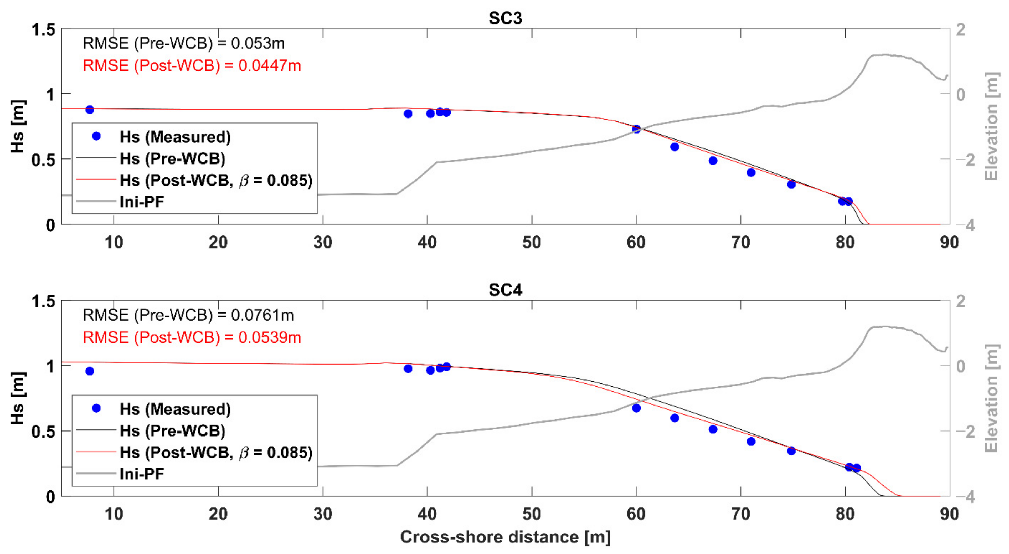
  • The cross-shore wave transformation was calibrated by using the breaker slope coefficient (β = 0.085), which affects the shoreward shift in wave-induced setup and return flow, resulting in an improvement across inner-surf zone in spite of there being no influence before the wave breaking.
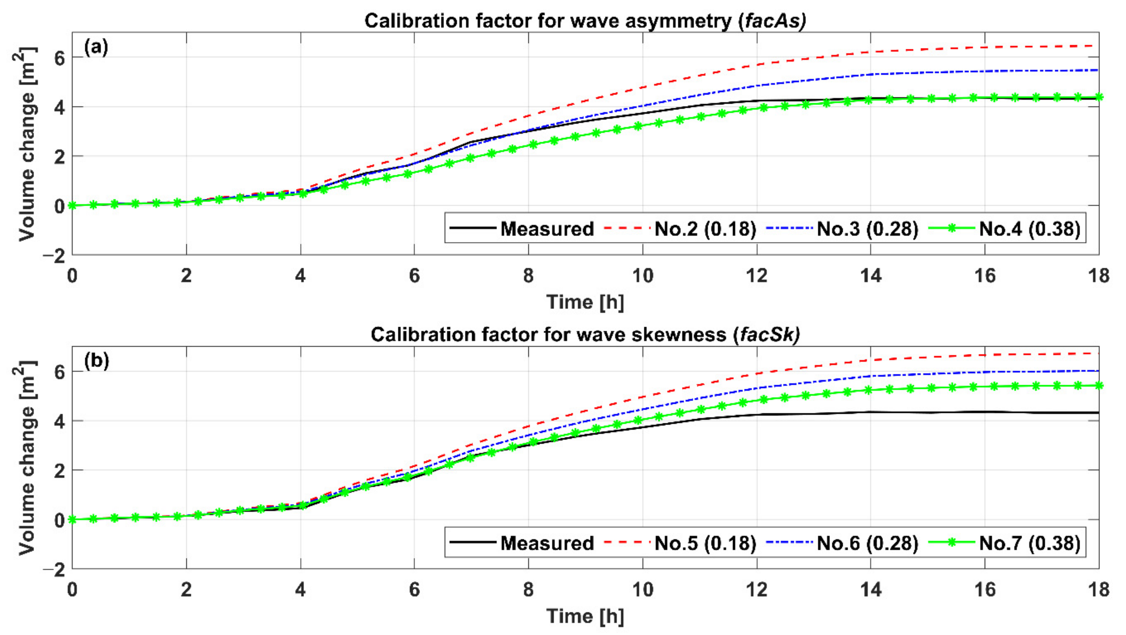
  • Wave skewness (facSk = 0.31) and asymmetry (facAs = 0.21) were used to calibrate dune profile simulation results in terms of wave nonlinearity and onshore sediment transport based on WTI setting. Because the wave skewness and asymmetry are closely related to wave nonlinearity, these parameters are sensitive to the bottom slope and wave spectral shape. Therefore, these parameters should be carefully calibrated in sand bar effect dominant cases.
  • The new coefficient (bermslope) in XBeachX was tested and calibrated by comparing it with the experimental results. The BSS value was the highest when the bermslope was 0.11. As a result, the foredune slope simulation was improved compared with the results from the previous studies.
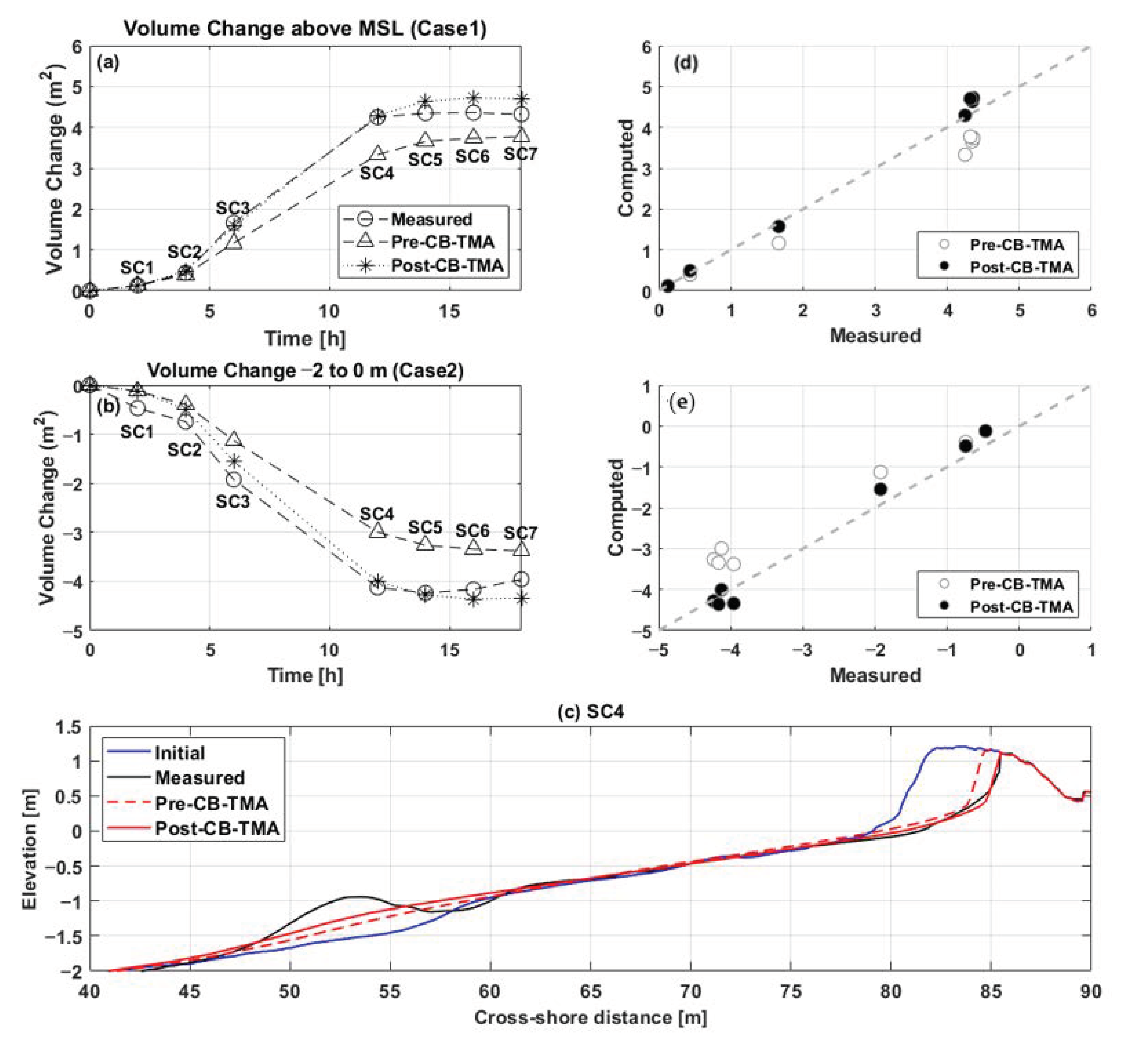
  • The simulation results with two supplementary validation cases by using four calibrated coefficients were significantly improved in terms of wave transformation, bermslope, and foredune erosion, while all simulation results of the underwater sand bar were still poor.
The present study calibrated the model with two steps in the morphodynamic calibration: (1) wave nonlinearity parameters (wave skewness and asymmetry); and (2) the beach slope parameter in the lower swash zone (bermslope). However, since these parameters might be interrelated, the model can be calibrated with the combination of the three parameters, simultaneously.
Even if the simulation results of the total erosion volume in both the dune area and the underwater region showed a good agreement, the local sand bar evolution was still not successfully simulated by XBeachX. Because XBeachX is a depth-averaged model where the horizontal wave velocity and undertow are considered vertically uniform, there can be limitations in local sand bar evolution simulation. Therefore, the adjustment of the vertical profile of horizontal velocity in the boundary layer may improve this simulation. Besides, spatial variation of sand distribution and the friction coefficient in the model should be studied to improve the model performance in terms of underwater sand bar evolution. The calibrated model set up in this study should also be validated using field observation data. Additionally, the model should be validated by using the experimental data of underwater hydrodynamics including the sand bar location.

Author Contributions

Conceptualization, K.D. and S.S.; methodology, H.J. and K.D.; software, H.J.; validation, H.J.; formal analysis, H.J.; investigation, H.J. and K.D.; resources, D.C.; data curation, S.S.; writing—original draft preparation, H.J., K.D. and S.S.; writing—review and editing, H.J., K.D., S.S. and D.C.; visualization, H.J.; supervision, K.D. and S.S.; project administration, K.D. and S.S.; funding acquisition, K.D. and S.S. All authors have read and agreed to the published version of the manuscript.

Funding

This research was partly supported by the project titled ‘Practical Technologies for Coastal Erosion Control and Countermeasure’, funded by the Ministry of Oceans and Fisheries, Korea (20180404) and by the National Research Foundation of Korea (NRF-2019R1C1C1003160).

Acknowledgments

The authors are thankful to Maddux and Ruggiero for providing their experimental data.

Conflicts of Interest

The authors declare no conflict of interest.

References

  1. Carter, R.W.G. Coastal Environments: An Introduction to the Physical, Ecological, and Cultural Systems of Coastlines; Academic Press: London, UK, 1988; pp. 301–333. [Google Scholar]
  2. Komar, P.D. Beach Process and Sedimentation, 2nd ed.; Prentice Hall: Hoboken, NJ, USA, 1998. [Google Scholar]
  3. Benimoff, A.I.; Fritz, W.J.; Kress, M. Chapter 3—Superstorm Sandy and Staten Island: Learning from the Past, Preparing for the Future; Bennington, J.B., Farmer, E.C., Eds.; Academic Press: Boston, MA, USA, 2015; pp. 21–40. [Google Scholar]
  4. Vigdor, J. The Economic Aftermath of Hurricane Katrina. J. Econ. Perspect. 2008, 22, 135–154. [Google Scholar] [CrossRef]
  5. Dissanayake, P.; Brown, J.; Wisse, P.; Karunarathna, H. Effects of storm clustering on beach/dune evolution. Mar. Geol. 2015, 370, 63–75. [Google Scholar] [CrossRef]
  6. McCall, R.T.; Van Thiel de Vries, J.S.M.; Plant, N.G.; Van Dongeren, A.R.; Roelvink, J.A.; Thompson, D.M.; Reniers, A.J.H.M. Two-dimensional time dependent hurricane overwash and erosion modeling at Santa Rosa Island. Coast. Eng. 2010, 57, 668–683. [Google Scholar] [CrossRef]
  7. Do, K.; Kobayashi, N.; Suh, K. Erosion of nourished Bethany beach in Delaware, USA. Coast. Eng. J. 2013, 56, 1450004. [Google Scholar] [CrossRef]
  8. Elsayed, S.M.; Oumeraci, H. Effect of beach slope and grain-stabilization on coastal sediment transport: An attempt to overcome the erosion overestimation by XBeach. Coast. Eng. 2017, 121, 179–196. [Google Scholar] [CrossRef] [Green Version]
  9. Do, K.; Shin, S.; Cox, D.; Yoo, J. Numerical Simulation and Large-Scale Physical Modelling of Coastal Sand Dune Erosion. J. Coast. Res. 2018, 85, 196–200. [Google Scholar] [CrossRef]
  10. Palmsten, M.L.; Splinter, K.D. Observations and simulations of wave runup during a laboratory dune erosion experiment. Coast. Eng. 2016, 115, 58–66. [Google Scholar] [CrossRef] [Green Version]
  11. Larson, M.; Kraus, N.C. SBEACH: Numerical Model for Simulating Storm-Induced Beach Change. Report 1, Empirical Foundation and Model Development. Technical Report CERC-89-9; U.S Army Engineer Waterways Experiment Station, Coastal Engineering Research Center: Washington, DC, USA, 1989.
  12. Kobayashi, N.; Farhadzadeh, A.; Melby, J.; Johnson, B.; Gravens, M. Wave overtopping of levees and overwash of dunes. J. Coast. Res. 2010, 2010, 888–900. [Google Scholar] [CrossRef]
  13. Roelvink, D.; Reniers, A.; van Dongeren, A.; van Thiel de Vries, J.; McCall, R.; Lescinski, J. Modelling storm impacts on beaches, dunes and barrier islands. Coast. Eng. 2009, 56, 1133–1152. [Google Scholar] [CrossRef]
  14. De Vet, P.L.M.; McCall, R.T.; Den Bien, J.P.; Stive, M.J.F.; Van Ormondt, M. Modelling Dune Erosion, Overwash and Breaching at Fire Island (Ny) during Hurricane Sandy. In Proceedings of the Coastal Sediment 2015, San Diego, CA, USA, 11–15 May 2015; pp. 1–10. [Google Scholar] [CrossRef] [Green Version]
  15. De Vet, P.L.M. Modelling sediment Transport and Morphology during Overwash and Breaching Events. Master’s Thesis, Delft University of Technology, Delft, The Netherlands, 28 July 2014. [Google Scholar]
  16. Brinkkemper, J.A. Modeling the cross-Shore Evolution of Asymmetry and Skewness of surface Gravity Waves Propagating over a natural Intertidal Sandbar. Master’s Thesis, Utrecht University, Utrecht, The Netherlands, 11 February 2013. [Google Scholar]
  17. van Geer, P.; den Bieman, J.; Hoonhout, B.; Boers, M. XBeach 1D—Probabilistic model: ADIS, Settings, Model uncertainty and Graphical User Interface. Tech. Rep. 2015, 18, 1209436. [Google Scholar]
  18. Roelvink, D.; Costas, S. Beach berms as an essential link between subaqueous and subaerial beach/dune profiles. Geo-Temas 2017, 17, 79–82. [Google Scholar]
  19. Roelvink, D.; Costas, S. Coupling nearshore and aeolian processes: XBeach and duna process-based models. Environ. Model. Softw. 2019, 115, 98–112. [Google Scholar] [CrossRef]
  20. Hughes, S.A. The TMA shallow-water spectrum description and applications. In Tech. Report CERC-84-7; US Army Corps of Engineers: Norfolk, VA, USA, 1984. [Google Scholar]
  21. Hasselmann, K.; Barnett, T.P.; Bouws, E.; Carlson, H.; Carwright, D.E.; Enke, K.; Ewing, J.A.; Gienapp, H.; Hasselmann, D.E.; Kruseman, P.; et al. Measurements of wind-wave growth and swell decay during the Joint North Sea Wave Project (JONSWAP). Dtsch. Hydrogr. Z. 1973, 8, 1–95. [Google Scholar]
  22. Maddux, T.B.; Ruggiero, P.; Palmsten, M.; Holman, R.; Cox, D.T. Laboratory Observations of Dune Erosion; AGU Fall Meeting (Poster): San Diego, CA, USA, 2006. [Google Scholar]
  23. Lashley, C.H.; Roelvink, D.; van Dongeren, A.; Buckley, M.L.; Lowe, R.J. Nonhydrostatic and surfbeat model predictions of extreme wave run-up in fringing reef environments. Coast. Eng. 2018, 137, 11–27. [Google Scholar] [CrossRef] [Green Version]
  24. Roelvink, D.; McCall, R.; Mehvar, S.; Nederhoff, K.; Dastgheib, A. Improving predictions of swash dynamics in XBeach: The role of groupiness and incident-band runup. Coast. Eng. 2018, 134, 103–123. [Google Scholar] [CrossRef]
  25. Lashley, C.H.; Bertin, X.; Roelvink, D.; Arnaud, G. Contribution of infragravity waves to run-up and overwash in the pertuis breton embayment (France). J. Mar. Sci. Eng. 2019, 7, 205. [Google Scholar] [CrossRef] [Green Version]
  26. Dissanayake, P.; Brown, J.; Karunarathna, H. Modelling storm-induced beach/dune evolution: Sefton coast, Liverpool Bay, UK. Mar. Geol. 2014, 357, 225–242. [Google Scholar] [CrossRef] [Green Version]
  27. Introduction—XBeach v.1.23.5741 Documentation. Available online: https://xbeach.readthedocs.io/en/latest/xbeach_manual.html (accessed on 9 May 2021).
  28. Rafati, Y.; Hsu, T.J.; Elgar, S.; Raubenheimer, B.; Quataert, E.; van Dongeren, A. Modeling the hydrodynamics and morphodynamics of sandbar migration events. Coast. Eng. 2021, 166, 103885. [Google Scholar] [CrossRef]
  29. Kalligeris, N.; Smit, P.; Ludka, B.C.; Guza, R.T.; Gallien, T.W. Calibration and assessment of process-based numerical models for beach profile evolution in southern California. Coast. Eng. 2020, 158, 103650. [Google Scholar] [CrossRef] [Green Version]
  30. Simmons, J.A.; Harley, M.D.; Marshall, L.A.; Turner, I.L.; Splinter, K.D.; Cox, R.J. Calibrating and assessing uncertainty in coastal numerical models. Coast. Eng. 2017, 125, 28–41. [Google Scholar] [CrossRef]
  31. Zimmermann, N.; Trouw, K.; De Maerschalck, B.; Toro, F.; Delgado, R.; Verwaest, T.; Mostaert, F. Scientic Support Regarding Hydrodynamics and Sand Transport in the Coastal Zone Evaluation of XBeach for Long Term Cross-Shore Modelling; Technical Report; Flanders Hydraulic Research: Antwerp, Belgium, 2015. [Google Scholar]
  32. van Rijn, L.C.; Wasltra, D.J.R.; Grasmeijer, B.; Sutherland, J.; Pan, S.; Sierra, J.P. The predictability of cross-shore bed evolution of sandy beaches at the time scale of storms and seasons using process-based profile models. Coast. Eng. 2003, 47, 295–327. [Google Scholar] [CrossRef]
  33. Walstra, D.J.R.; Van Rijn, L.C.; Van Ormondt, M.; Brière, C.; Talmon, A.M. The effects of bed slope and wave skewness on sediment transport and morphology. In Proceedings of the Sixth International Symposium on Coastal Engineering and Science of Coastal Sediment Process, New Orleans, LA, USA, 13–17 May 2007. [Google Scholar] [CrossRef] [Green Version]
  34. Shin, S.; Kim, J.; Yoo, J.; Do, K.; Chang, T.; Kim, J. Dune erosion and sand bar migration during a storm event: Large-scale wave flume test and numerical simulation. In Proceedings of the Virtual International Conference on Coastal Engineering (vICCE), Online, 6–9 October 2020. [Google Scholar]
  35. Bretschneider, C.L. Significant Waves and Wave Spectrum; Ocean Industry: St. Lawrence River, NY, USA, 1968; pp. 40–46. [Google Scholar]
  36. Mitsuyasu, H. On the Growth of the Spectrum of Wind-Generated Waves. Coast. Eng. Japan 1970, 13, 1–14. [Google Scholar] [CrossRef]
Figure 1. Top view (upper panel) and side view (lower panel) of the flume and instrument setup. Open circles and solid lines: resistance-type wave gauges; yellow squares: ultrasonic wave gauges; black solid line: initial beach profile; red solid line: final beach profile.
Jmse 09 00635 g001
Figure 2. Flow chart of the calibration procedure in the present study: Hydrodynamic and morphodynamic calibration subcategorize one and two steps each, resulting in three sequential adjustments.
Jmse 09 00635 g002
Figure 3. Hs of pre and post (optimized) WCB after storm conditions (SC3 and SC4): Measured (blue filled circle), pre- WCB (solid black line), and post-WCB (solid red line, beta = 0.085), and initial profile (solid gray line).
Jmse 09 00635 g003
Figure 4. Time-varying volume changes above mean sea level under (a) facSk = 0.13 with varying facAs (0.18, 0.28, and 0.38), (b) facAs = 0.13 with varying facSk (0.18, 0.28, and 0.38): No. (simulation number in Table 3), Measured (black solid line), 0.18 (red dashed line), 0.28 (blue dash-single dotted line), and 0.38 (green solid line with star shapes).
Jmse 09 00635 g004
Figure 5. Brier-Skill-Score for computed final profile of SC3 and SC4: No. (simulation number in Table 3), Case1 (blue circle)—bed level above 0 m (MSL, Mean Sea level) and Case2 (red circle)—bed level between −2 and 0 m.
Jmse 09 00635 g005
Figure 6. Comparison of initial, measured and computed final profiles applied to wave calibration (WCB) and wave shape calibration (facSK = 0.31 and facAs = 0.21) for SC3, SC4, and SC5.
Jmse 09 00635 g006
Figure 7. Initial, measured, and computed final profile for SC4: (a) slope of swash zone: measured profile (1:7) and computed profile (1:10); (b) bermslope (BS) effect.
Jmse 09 00635 g007
Figure 8. Measured and computed (pre and post-CB-TMA) volume changes of final profiles throughout the entire scenario (ad) and profiles after SC4 (e): volume changes (a) above MSL and (c) between −2 and 0 m and correlation (b) above MSL and (d) between −2 and 0.
Jmse 09 00635 g008
Figure 9. Initial (black), final measured and computed profile (blue and red, respectively), and significant wave height (gray solid line: simulated, red circle: measured) of two experiments (upper panel: OSU2019, lower panel: HYU2019).
Jmse 09 00635 g009
Table 1. Incident wave and water level conditions for each step. Hs, Tp, and WL denote significant wave height, peak period, and water level, respectively [9].
CaseHs (m)Tp (s)WL (m)
Initial0.254.903.96
SC10.502.044.00
SC20.673.064.05
SC31.004.804.09
SC41.174.904.13
SC51.004.904.09
SC60.674.904.05
SC70.504.904.00
Recovery0.254.903.96
Table 2. Summarized general input information for numerical setup provided by the previous study [9].
Input for SetupGrid PointGrid Resolution D 50 PorositySpecific Gravity
Values126Non-equidistant
(0.15 to 2 m)
0.2 mm0.42.65
Table 3. facSk and facAs lists during XBeach modeling: No. (simulation number), Sk (facSk), and As (facAs).
No.123456789101112 1131415
Sk0.130.130.130.130.180.280.380.220.240.260.280.310.330.350.37
As0.130.180.280.380.130.130.130.140.160.180.200.210.230.250.27
1 Optimized calibration parameter, which is 0.989 of BSS above mean sea level for SC4.
Publisher’s Note: MDPI stays neutral with regard to jurisdictional claims in published maps and institutional affiliations.

