VPP Coupling High-Fidelity Analyses and Analytical Formulations for Multihulls Sails and Appendages Optimization

Abstract

A procedure for the optimization of a catamaran’s sail plan able to provide a preliminary optimal appendages configuration is described. The method integrates a sail parametric CAD model, an automatic computational domain generator and a Velocity Prediction Program (VPP) based on a combination of sail RANS computations and analytical models. The sailing speed and course angle are obtained, with an iterative process, solving the forces and moment equilibrium system of equations. Analytical formulations for the hull forces were developed and tuned against a matrix of CFD solutions. The appendages aerodynamic polars are estimated by applying preliminary design criteria from aerospace literature. The procedure permits us to find the combination of appendages configuration, rudders setting, sail planform, shape and trim that maximise the VMG (Velocity Made Good). Two versions of the sail analysis module were implemented: one adopting commercial software and one based on the use of only Open-Source codes. The solutions of the two modules were compared to evaluate advantages and limitations of the two approaches.

1. Introduction

A sailing boat is a mechanical system in which several forces and moments act in a complex environment whose static and dynamic equilibrium affect the overall performance. The sailing speed depends on the boat characteristics and on the sails performances with a mechanism that requires several aspects of physics involved to be opportunely modelled. For this reason, yacht design should be faced within so-called Velocity Prediction Program (VPP) environments [1]. VPPs are procedures that evaluate the global equilibrium of the system balancing hull and sail forces. Their accuracy is strongly related to the accuracy of the model adopted to estimate the forces [2]. The typical approaches to feed the models are the generation of experimental databases [3,4] or the integration of CFD (Computational Fluid Dynamic) computations [5]. Adopting numerical flow solutions, however, can significantly increase the cost of computations leading to procedures that are not compatible with the practical requirements of design especially in the preliminary sizing phases. The identification of the most opportune compromise between accuracy and computational requirements is the winning strategy to develop efficient design tools. The adoption of a combination of surrogate models and available sails data to reduce the calculation requirements in VPPs is proposed in [6]. In [7] analytical formulations for sail aerodynamics have also been described. In [8], the data deriving from experiments and computations are used to develop a VPP for the Olympic Nacra 17 foiling catamaran. In some cases, as for instance in foiling vessels, the sailing dynamic stability plays a crucial role. In [9], the dynamic stability is included in a VPP developed for the International Moth dinghy. In [10], such aspect is studied for a 16-foot foiling catamaran.

The method here proposed integrates a parametric geometry model of the sail plan, an automatic computational domain generator and a VPP based on a combination of CFD computations and analytical models. Sailing speed and course angle are obtained, with an iterative process, solving the forces and moments equilibrium system of equations. The hull forces are modelled by empirical analytical formulations whose coefficients are tuned against a matrix of known solutions of the isolated demihull. This model provides a very fast evaluation of the forces at a given velocity, displacement and leeway angle. Dagger boards and rudders are modelled as wings. Their aerodynamic polars are estimated applying preliminary design criteria from the aerospace literature. The closure of the equations system is assured by the sail forces and the position of the aerodynamic centre of effort provided by RANS (Reynolds Averaged Navier–Stokes) computations. The VPP is integrated in a numerical optimization environment which permits to find the sail planform, shape and trim that, in combination to a preliminary evaluation of the optimal appendages configuration and rudders setting, maximise the boat VMG (Velocity Made Good). The test case used for the development of the method is a Classic A-Class catamaran.

Part of the work reported in this paper was funded within the 4th EU PRACE’s SHAPE programme. At the end of the project a technical report was produced and made available online [11]. The present work was inspired by that report from which it differs for a deeper description of the implemented modules with particular focus on the VPP.

The paper is divided into three parts: the first introduces the VPP that couples the analytical model of the boat to the sail RANS solution, the second one describes the development of the modules of the optimization environment and the last one compares the solutions of two versions of the sail analysis model applied to a simple A-Cat sail optimization problem. The two proposed CFD modules differ in the numerical tools used to implement them. One was developed adopting well-known commercial software while the other is based on Open-Source codes. The integration of the latter model allows to propose a design tool completely free from commercial licenses (the VPP and the parametric CAD model of the sail are already based on Open-Source software) with a clear advantage in economic terms. Nevertheless, its accuracy and the complexity related to its implementation in an optimization environment should be verified case by case. The comparison here reported was planned with this purpose.

2. Performance Prediction Model

A boat model, fully based on analytical formulations, is proposed. The objective is to provide a very fast and versatile tool able to estimate the boat characteristics with an accuracy acceptable in the preliminary development phase and suitable for an optimization environment. The strength of this approach is the capability to easily parametrise several aspects of the boat components providing the possibility to involve in the optimization a wide range of design variables as chord, draft, twist, setting, airfoil and planform of the appendages. The boat model is developed in form of a Scilab function [12] able to interact, in a comparative iterative process within the equilibrium equations system, with the sail RANS aerodynamic solution to constitute a VPP.

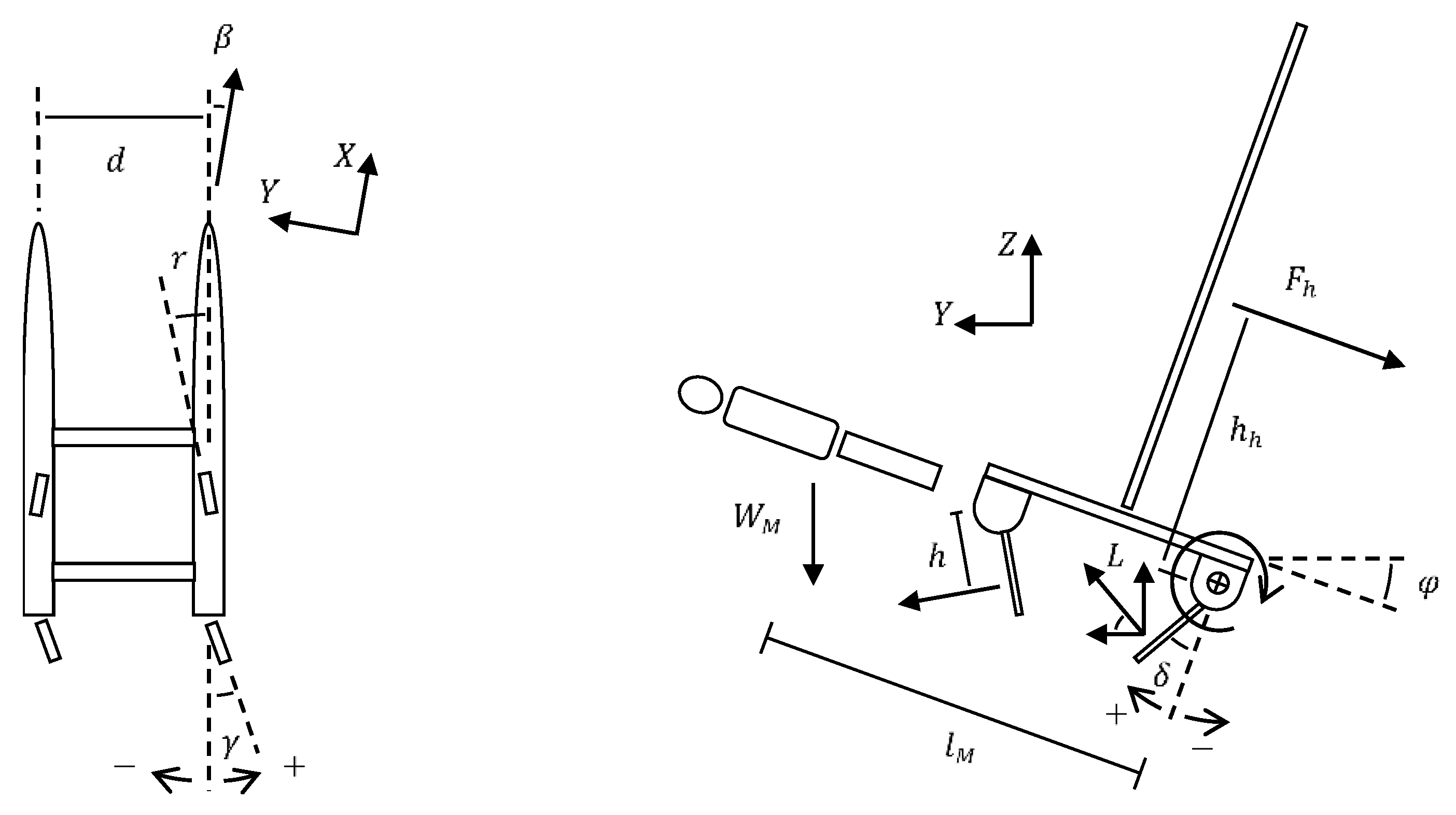
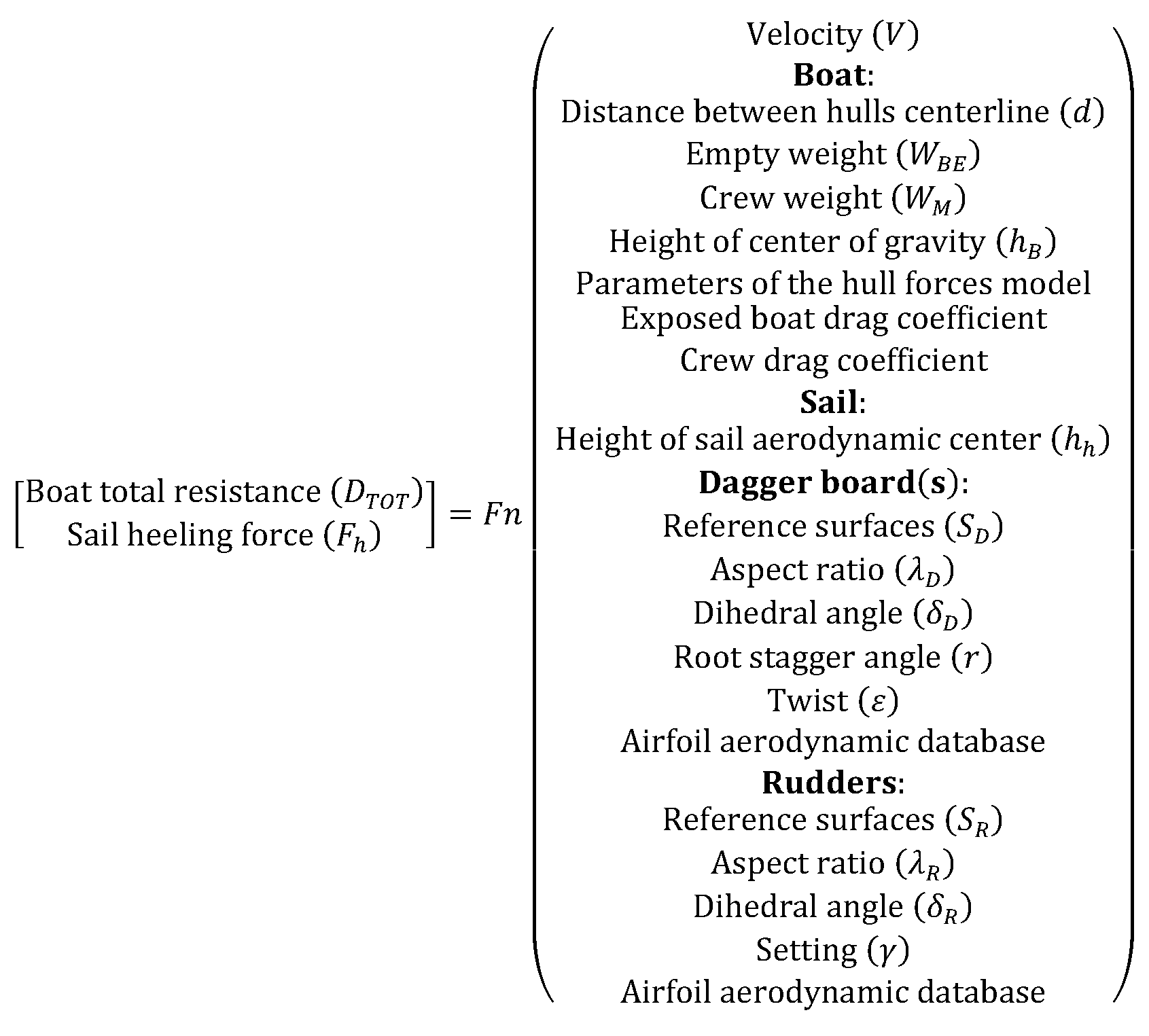
2.1. Boat Global Forces and Moment Equilibrium

Figure 1 reports the orientation of the adopted reference frame and summarises the forces acting on the boat.

The forces equilibrium equations of the complete boat, referred to a frame with the $X$ axis aligned with the sailing direction and the $Z$ axis perpendicular to the water plane, are:

Xequilibrium

$$D_{TOT}=D_{D_D}+D_{D_U}+D_{R_D}+D_{R_U}+D_H+D_{M_x}+D_{B_x}=F_t$$

(1)

$D$ refers to drag, the subscripts ${*}_{D_D}$, ${*}_{D_U}$, ${*}_{R_D}$ and ${*}_{R_U}$ refer, respectively, to downwind dagger board, upwind dagger board, downwind rudder and upwind rudder. $D_H$ is the demihull resistance, $D_{M_x}$ and $D_{B_x}$ are the aerodynamic drag component along the $X$ direction, respectively, of the crew and the boat. $F_t$ is the thrust force of the sail.

$\mathit{Y}$equilibrium (assuming to neglect the lift generated by the boat)

$$F_h\mathit{cos}\phi +D_{M_y}+D_{B_y}=L_{D_D}\mathit{cos}\left(\phi +{\delta }_D\right)+L_{D_U}\mathit{cos}\left(\phi -{\delta }_D\right)+L_{R_D}\mathit{cos}\left(\phi +{\delta }_R\right)+L_{R_U}\mathit{cos}\left(\phi -{\delta }_R\right)+L_H$$

(2)

$F_h$ is the sail heeling force, $\phi$ is the heeling angle, $D_{M_y}$ and $D_{B_y}$ are the aerodynamic drag component along the $Y$ direction, respectively, of the crew and the boat. $L$ refers to lift force, $\delta$ refers to the appendages dihedral angle and $L_H$ is the side force generated by the demihull. The subscripts ${*}_D$ and ${*}_R$ refer to dagger boards and rudders.

$\mathit{Z}$equilibrium

$$W_M+W_{BE}+F_h\mathit{sin}\phi =W_{BO}+L_{D_D}\mathit{sin}\left(\phi +{\delta }_D\right)+L_{D_U}\mathit{sin}\left(\phi -{\delta }_D\right)+L_{R_D}\mathit{sin}\left(\phi +{\delta }_R\right)+L_{R_U}\mathit{sin}\left(\phi -{\delta }_R\right)$$

(3)

$W_M$ is the crew weight, $W_{BE}$ is the boat empty weight and $W_{BO}$ is the boat operative weight.

The moment equilibrium along the $X$ axis and around the centre of buoyancy of the downwind hull gives:

${\mathit{M}}_{\mathit{X}}$equilibrium

$$\begin{gathered} W_{BE}\frac{d}{2}\mathit{cos}\phi +W_M{l}_M\mathit{cos}\phi =W_{BE}{h}_g\mathit{sin}\phi +F_h{h}_h+L_{D_D}{h}_{D_D}+L_{D_U}\left(h_{D_U}-d\mathit{sin}{\delta }_D\right)+L_{R_D}{h}_{R_D} \\ +L_{R_U}\left(h_{R_U}-d\mathit{sin}{\delta }_R\right)+W_{BE}{h}_B\mathit{sin}\phi \end{gathered}$$

(4)

where the left-hand side of the equation represents the maximum possible righting moment with the helmsman at trapeze. The term $h_h$ is the height of the sail centre of effort and $h_g$ is the height of the boat centre of gravity. The other terms $h$ refer to the arm of the resulting force relative to the element identified by the subscripts.

It was decided to not involve the yaw and pitching moment equilibrium in the system. The first in general impacts the rudder angle while the latter mainly influences the hull longitudinal setting. Both parameters can be controlled with an opportune sail rig/appendage centring and crew position. In more detail, the idea is to avoid including the yaw equilibrium, for which the variables would be the relative mast/daggerboard positions, and to include the rudder setting as variable of design. Its most opportune setting can be obtained as output of the optimization and operatively achieved by positioning the mast and the appendages in a location that allows sailing with the required rudder setting. The option to avoid solving the pitching moment equilibrium might appear not opportune in case of very slender hulls such as the catamaran’s ones. In our case, nevertheless, the extremely light empty weight of the boat (comparable with the weight of the crew) allows to force the longitudinal attitude in all sailing conditions controlling the position of the crew without the requirement of including the longitudinal degree of freedom in the system. As it was done for the rudder, the longitudinal setting can be imposed as variable of design without deriving it as consequence of the equilibrium. In the view of developing a static VPP, the assumption to neglect the two additional equilibrium equations is considered acceptable for the presented application.

2.1.1. Hull Forces Modelling

A large amount of literature is available, and several strategies are offered to model a traditional monohull sailing yachts, from databases solutions to accurate regression based polynomial expressions [13,14]. Such methods are not valid in case of fast catamarans hulls although experiments on slender bodies, both in calm water and head waves, are available to support the development of analytical models [15]. A significant contribution on this topic is provided by the Molland’s work [16]. Nevertheless, the documented correlations inspired the develop of simplified formulations customised to a typical A-Class cat hull shape whose coefficients are to be tuned knowing a limited set of forces data of the hull to be modelled. The formulations were developed by a comparison with a wide matrix of data of a reference hull at several attitudes and leeway angles. The reference database was obtained by RANS analyses in place of experimental measurements. The literature confirms, in fact, the confidence in the accuracy of CFD solutions for both displacing and planning hulls [17,18]. The adopted base of validation of the analytical model is the demihull of a Flyer S A-Class catamaran (Figure 2).

Two formulations were developed for hull side force and for drag. To estimate the hull side force (force laying in a plane parallel to the water plane and normal to the sailing direction), the bare hull is modelled as a lifting body as follows:

$$L_H=\frac{1}{2}{\rho }_w{V}^2{S}_H\frac{\partial C_{L_H}}{\partial \beta }\beta$$

(5)

where ${\rho }_w$ is the sea water density, $V$ is the boat velocity and $\beta$ is the leeway angle. The reference surface $S_H$ is the side projection, on the symmetry plane, of the submerged part of the demihull and changes with displacement. It is modelled, for a typical A-Class hull shape, by two formulations approximating a set of values computed by a CAD system and valid before and after a defined operative weight $W_{B{O}_0}$:

$$S_H=\{\begin{array}{cc}\hfill \left(k_{S_H{}_1}{W}_{B{O}_0}+k_{S_H{}_2}\right){\left(\frac{W_{BO}}{W_{B{O}_0}}\right)}^{{\tau }_{S_H}}, & W_{BO}<W_{B{O}_0}\\ \hfill k_{S_H{}_1}{W}_{BO}+k_{S_H{}_2}, & W_{BO}\ge W_{B{O}_0}\end{array}$$

(6)

The coefficients $k_{S_H{}_1}$ and $k_{S_H{}_2}$ are computed knowing two surface values in the linear region. ${\tau }_{S_H}$ is estimated adding a known value at an operative weight lower than $W_{B{O}_0}$.

According to the matrix of CFD solutions of the reference demihull, the slope of the side force curve $\frac{\partial C_{L_H}}{\partial \beta }$ linearly change with the displacement. Nevertheless, also a non-linear relation with the velocity (Reynolds effect) and the leeway angle was observed. To account for those effects the developed formulation contains exponential expressions of the two parameters:

$$\frac{\partial C_{L_H}}{\partial \beta }=V^{{\tau }_{H_1}}{\beta }^{{\tau }_{H_2}}\left(k_H{}_1{W}_{BO}+k_H{}_2\right)$$

(7)

The parameters $k_H{}_1$, $k_H{}_2$, ${\tau }_{H_1}$ and ${\tau }_{H_2}$ are tuned against the known hull data. The graphs in Figure 3 compare the analytical solutions at two velocities and three leeway angles with the reference CFD database.

The bare demihull total resistance is expressed by:

$$D_H=\frac{1}{2}{\rho }_w{V}^2{S}_{wet}{C}_T$$

(8)

The reference wet surface $S_{wet}$ depends on the operative weight and is modelled with two formulations similar to the ones adopted to model $S_H$. The values to be approximated are computed by CAD. The model estimates the surface value starting from zero displacement in order to provide the procedure the capability to analyse also configurations in which the lifting contributions of the foils are predominant to the hull forces.

$$S_{wet}=\{\begin{array}{cc}\hfill \left(k_{S_w{}_1}{W}_{B{O}_0}+k_{S_w{}_2}\right){\left(\frac{W_{BO}}{W_{B{O}_0}}\right)}^{{\tau }_{S_w}}, & W_{BO}<W_{B{O}_0}\\ \hfill k_{S_w{}_1}{W}_{BO}+k_{S_w{}_2}, & W_{BO}\ge W_{B{O}_0}\end{array}$$

(9)

The terms $k_{S_w{}_1}$, $k_{S_w{}_2}$ and ${\tau }_{S_w}$ are found knowing the hull wet surface at two displacement values in the linear and one in the non-linear region. Figure 4 reports the comparison between the wet surface modelled by the developed analytical formulation and the values of the reference hull computed by CAD.

The total resistance coefficient is modelled as a combination of a friction and a residuary component [19]:

$$C_T=\left(1+k\right)C_f+C_w$$

(10)

The form factor $\left(1+k\right)$ accounts for the over velocity generated by the thick shape of the body [20]. Its value is evaluated from literature or from a known bare hull drag value. The skin friction coefficient is estimated according to the ITTC-57 friction line expression [21]:

$$C_f=\frac{0.075}{{\left(log{R}_N-2\right)}^2}$$

(11)

where $R_N=\frac{V{L}_{wl}}{\nu }$ is the Reynolds number referred to the hull waterline length. Good agreement with CFD computations was observed (Figure 5) adopting as $L_{wl}$ the full length of the hull (modern A-Cat hulls have an inversed bow shape).

A significant simplification was chosen to model the residuary drag coefficient $C_w$. A combination of two quadratic formulations with Froude number, for speeds lower and higher than a critical value and linearly function of the operative weight, was adopted:

$$C_w=\{\begin{array}{cc}\hfill (W_{BO}+w_w)(k_{w_1}+\frac{k_{w2}}{F_{N{c}_r}}+\frac{k_{w3}}{{F_{N{c}_r}}^2}){F_N}^2,& F_N<F_{N{c}_r}\\ \hfill (W_{BO}+w_w\left)\right(k_{w_1}{F_N}^2+(k_{w_2}{F}_N+k_{w_3}),& F_N\ge F_{N{c}_r}\end{array}$$

(12)

The factor $\left(W_{BO}+w_w\right)$ accounts for the dependency from the operative weight and is tuned by the term $w_w$. The values of $w_w$, $k_{w_1}$, $k_{w_2}$ and $k_{w_3}$ are to be tuned against the matrix of the known demihull solutions. If a large database of hull solution is available, the combination of values that best match the data might be identified with a trial-and-error procedure. The values adopted for the reference hull were identified by a numerical optimization procedure that converges toward the combination of values that minimize the absolute difference between the analytical formulation and the computed CFD values. To further best match the data, the boundary Froude number might differ from the theoretical critical value of 0.4 referred to the waterline length. The Figure 6 compares the solutions of the analytical wave drag model with the CFD solutions of the reference hull at two operative weights.

Figure 7 compares the computed (by CFD) and the modelled (by the developed analytical models) viscous and residuary drag of the reference hull. It is evident how the viscous component is dominant in most of typical A-Cat speed range. Therefore, the relative roughness of the wave drag model poorly affect the accuracy of the total hull drag estimation.

An additional factor that accounts for the drag increase due to the leeway angle was also included. Such dependency was assumed to be quadratic with leeway angle. From the CFD computations it was also observed to be linearly dependent to the operative weight and exponentially to velocity. The proposed factor to be included is:

$$1+k_{\beta }{V}^{{\tau }_{\beta }}\left(W_{BO}+w_{\beta }\right){\beta }^2$$

(13)

The terms $k_{\beta }$, ${\tau }_{\beta }$ and $w_{\beta }$ are tuned against the known hull solutions. The final analytical drag formulation assumes then the form:

$$D_H=\frac{1}{2}{\rho }_w{V}^2{S}_{wet}\left[\left(1+k\right)C_f+C_w\right]\left[1+k_{\beta }{V}^{{\tau }_{\beta }}\left(W_{BO}+w_{\beta }\right){\beta }^2\right]$$

(14)

Figure 8 compares, for the reference hull, the modelled hull drag increase due to the leeway angle with the CFD computations at two velocities.

The analytical formulations can be tuned to model new hulls knowing a total of three CAD measurements at three displacements and a minimum of six CFD solutions or experimental forces measurements at two values of velocities, attitudes and leeway angles. The coefficients adopted to model the reference Flyer S demihull forces are listed in

Table 1. Values of the parameters adopted to model the Flyer S demihull forces.

Reference Surfaces	Side Force	Wave Drag	Leeway Drag
$k_{S_H{}_1}$ = 0.00437	$k_H{}_1$ = 6 × 10−7	$w_w$ = 80 kg	$k_{\beta }$ = 2 × 10−6
$k_{S_H{}_2}$ = 0.07	$k_H{}_2$ = 1.3 × 10−4	$k_{w_1}$ = 2.16 × 10−6	${\tau }_{\beta }$ = 1.5
${\tau }_{S_H}$ = 0.83	${\tau }_{H_1}$ = 1.3	$k_{w_2}$ = −8.3 × 10−6	$w_{\beta }$ = 400 kg
$k_{S_w{}_1}$ = 0.00876	${\tau }_{H_2}$ = 0.2	$k_{w_3}$ = 9 × 10−6
$k_{S_w{}_2}$ = 0.95
${\tau }_{S_w}$ = 0.5	shape factor $k$ = 0.01
$W_{B{O}_0}$ = 94 kg

.

2.1.2. Appendages Forces Modelling

Dagger boards and rudders are modelled as wings. Their aerodynamic polars are estimated applying preliminarily design criteria from literature. The formulation for lift is:

$$L=\frac{1}{2}{\rho }_w{V}_{eff}{}^{2}S{C}_L$$

(15)

The lift coefficient, in the linear region of the lift curve of a non-symmetric foil, can be expressed as:

$$C_L=\frac{\partial C_L}{\partial \alpha }{\alpha }_{eff}+C_{L0}$$

(16)

where $\frac{\partial C_L}{\partial \alpha }$ is the slope of the lift curve and $C_{L0}$ is the lift generated by the foil at zero incidence. The effective velocity $V_{eff}$ is the component of the boat velocity vector normal to the foil leading edge (for rectangular planform) and ${\alpha }_{eff}$ is its angle of incidence. $V_{eff}$ is the only velocity component responsible for the generation of lift (the friction contribution can be neglected). The spanwise component, in fact, does not affect the lift but only causes a shifting of the boundary layer [22]. From geometrical considerations it can be demonstrated that, for moderate values of the leeway angle, the effective velocity can be approximated to the boat speed:

$$V_{eff}\approx V$$

(17)

and the effective incidence can be approximated, for instance for the downwind appendage, to:

$${\alpha }_{eff}\approx \beta \mathit{cos}\left(\phi +{\delta }_D\right)$$

(18)

From the above considerations and referring to the Figure 1, the lift coefficients of dagger boards and rudders are then expressed in function of $\beta$ as follows:

$$\begin{array}{c}{C}_{L_{D_D}}={\left(\frac{\partial C_L}{\partial \alpha }\right)}_{D_D}\left[\beta \mathit{cos}\left(\phi +{\delta }_D\right)+r\right]+C_{L{0}_{D_D}}\\ C_{L_{D_U}}={\left(\frac{\partial C_L}{\partial \alpha }\right)}_{D_U}\left[\beta \mathit{cos}\left(\phi -{\delta }_D\right)-r\right]-C_{L{0}_{D_U}}\\ C_{L_{R_D}}={\left(\frac{\partial C_L}{\partial \alpha }\right)}_{R_D}\left[\beta \mathit{cos}\left(\phi +{\delta }_R\right)+\gamma \right]\\ C_{L_{R_U}}={\left(\frac{\partial C_L}{\partial \alpha }\right)}_{R_U}\left[\beta \mathit{cos}\left(\phi -{\delta }_R\right)+\gamma \right]\end{array}$$

(19)

The 3D lift curve slopes are estimated by empirical formulations used in aeronautics in the preliminary design phase [23]. Assuming a linear twist and constant airfoil section along the full span, it is modelled (with dimension $\raisebox{1ex}{$1$}\!\left/ \!\raisebox{-1ex}{$deg$}\right.$) as:

$$\frac{\partial C_L}{\partial \alpha }=f\frac{{\left(\frac{\partial C_l}{\partial \alpha }\right)}_{2D}\frac{b}{2p}}{1+57.3\frac{{\left(\frac{\partial C_l}{\partial \alpha }\right)}_{2D}\frac{b}{2p}}{\pi \lambda }}$$

(20)

The terms $p$ is the foil planform perimeter subtracting the root chord length, $b$ is the appendage draft and $\lambda$ the aspect ratio of the mirrored full span geometry. The term ${\left(\frac{\partial C_l}{\partial \alpha }\right)}_{2D}$ is the 2D lift curve slope of the adopted airfoil.

The dagger boards lift coefficients at zero incidence $C_{L{0}_D}$ are obtained solving the lift curve equations for $C_{L_D}=0$ (first two expressions of Equation (19)) substituting to the factor between squared brackets the 3D angle of incidence at which the foil generates zero lift that, for the downwind dagger board, for instance, is given by:

$${\alpha }_{C_{L0}}={\alpha }_{C_{L{0}_{2D}}}+J\epsilon -r$$

(21)

${\alpha }_{C_{L{0}_{2D}}}$ is the zero-lift incidence of the airfoil, $\epsilon$ is the foil twist and $r$ the root stagger angle.

The appendages drag formulation is:

$$D=\frac{1}{2}{\rho }_w{V}^{2}S{C}_D$$

(22)

where the drag coefficient $C_D$ is expressed in function of the lift coefficient.

$$C_D=C_{D0}+\frac{C_L{}^2}{\pi \lambda e}+C_L\epsilon {\left(\frac{\partial C_l}{\partial \alpha }\right)}_{2D}v+{\left[\epsilon {\left(\frac{\partial C_l}{\partial \alpha }\right)}_{2D}\right]}^{2}w$$

(23)

The 2D lift curve slope of the airfoil ${\left(\frac{\partial C_l}{\partial \alpha }\right)}_{2D}$ required in Equations (20) and (23), the zero lift incidence ${\alpha }_{C_{L{0}_{2D}}}$ of Equation (21), the drag at zero lift $C_{D0}$ in Equation (23) refer to the characteristics of the selected airfoil and can be provided in several ways. In the method described in this paper three options were implemented: they can be provided as an external experimental database, in a form of coefficients of analytical 2D polars or can be computed “on the fly” by a coupled panel/boundary layer code [24] in which the airfoil is parameterized by a NURBS control polygon or provided in formatted coordinates of points. The values of $f$ in Equation (20), $J$ in Equation (21), $e$, $v$ and $w$ in Equation (23) are reported in the literature as a function of aspect and taper ratio [25].

The analytical formulations above described are valid for isolated wings. The effect on rudders of the daggerboard downwash was considered moderate and neglected at this stage. From the downwash chart reported in [26], it was estimated that this approximation introduces uncertainness on the total drag in the order of fractions of percentage. Other phenomena such as wall interference, ventilation and the effects of the moderate curvature of Classic A-Cat daggerboards were also not considered. An activity to refine the models is on progress by fine tuning additional factors against an extended database of CFD solutions on hulls with appendages (Figure 9). For sail optimization purpose, nevertheless, moderate uncertainness in the accuracy of the VMG is not expected to invalidate the search direction of the shape that maximize the sail thrust.

Substituting the foils forces formulation in the equilibrium system of equations—Equations (1)–(4)—and including the hull side force model—Equation (5)—we obtain, assuming the boat velocity $V$ and the height of sail aerodynamic centre of effort $h_h$ to be given as input, a system of five equations and five unknowns ($D_{TOT}$, $F_H$, $W_{BO}$, $L_H$ and $\beta$). The solution of the equations system is implemented as a script function (written in Scilab) that produces as output the boat total resistance $D_{TOT}$ and the sail heeling force $F_H$ (which are the parameters to be compared with the CFD sail solutions) at a given speed $V$, centre of effort height $h_h$ and set of parameters characterising the boat configuration (Figure 10).

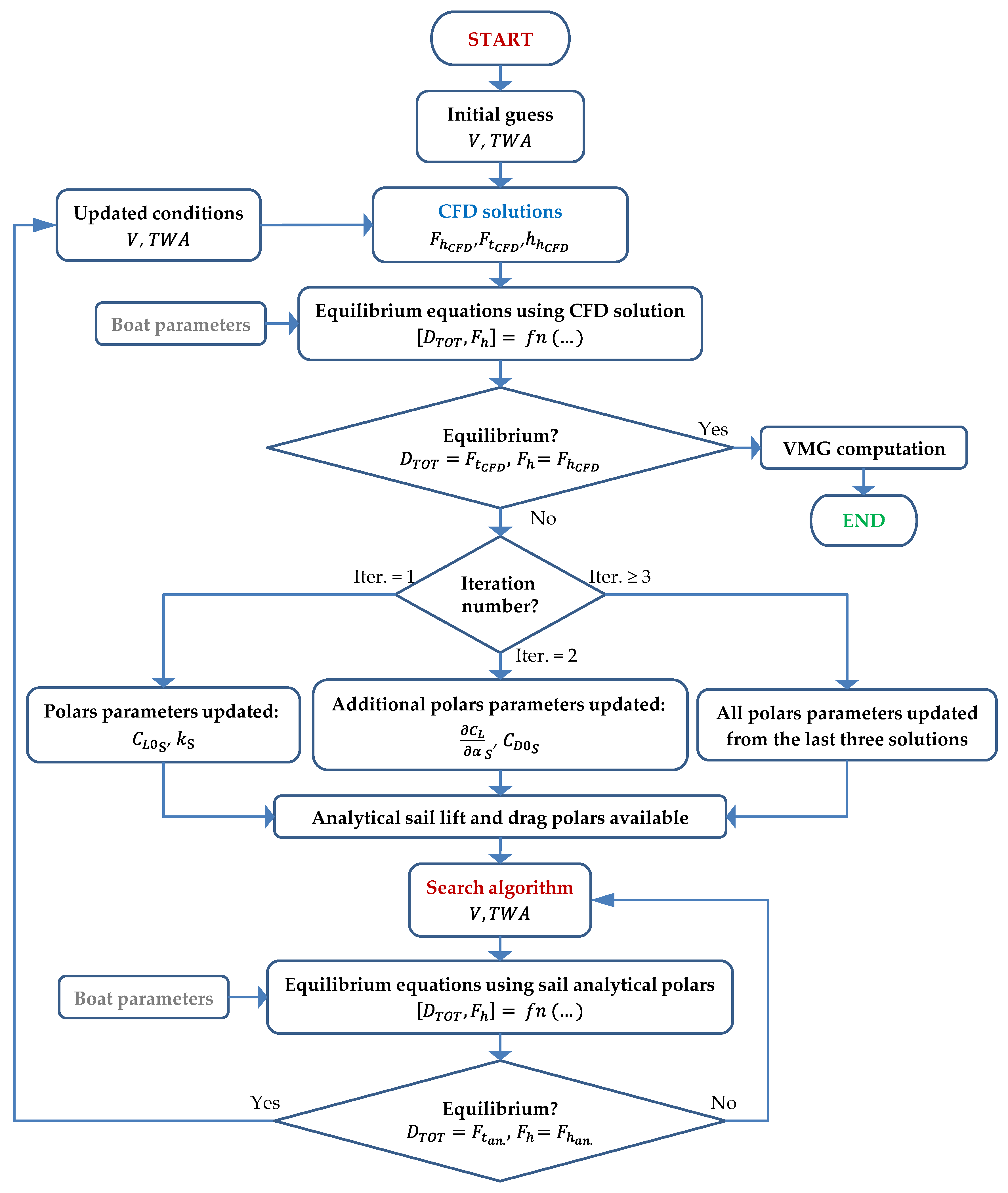
2.2. Closure of the Performance Solution Problem

No sail aerodynamic model is included in the function modelling the boat performance. As anticipated, it requires an input of two unknown parameters that are not related to the boat geometry or setting: the velocity of the boat $V$ and the height of the sail centre of effort $h_h$. The closure of the problem is provided, iterating with the CFD aerodynamic solution of the sail at fixed sailing conditions.

Figure 11 describes the workflow to estimate the VMG for a given combination of parameters characterising the boat configuration. The procedure begins guessing an initial sailing speed $V$ and course $TWA$. A CFD analysis, with the selected sail plan, shape and trim, is then run at these conditions. Sail forces and centre of effort are extracted and used to verify the equilibrium system. The verification consists in checking if the boat total resistance and the sail heeling force, computed by the analytical model for the given hull and appendage configuration, are equal, respectively, to the sail thrust force and the heeling force deriving from the CFD computation:

$$\{\begin{array}{c}{D}_{TOT}=F_t{}_{CFD}\\ F_h=F_h{}_{CFD}\end{array}$$

(24)

If the two solutions are different, new values of boat speed and true wind angle are selected. The CFD computation is restarted at the new conditions and the procedure is repeated until the equilibrium equations criteria are verified (within a prescribed tolerance). The VPP problem is completed with the production, as output, of the “Velocity Made Good” ($VMG=V\mathit{cos}TWA$), which represents the velocity of the boat toward the wind direction [27] with the selected sail geometry (considered rigid) and appendages.

To speed up the convergence of the VPP solution, the procedure of sailing conditions exploration was split into two nested cycles. The principle is to use an external loop, which involves the RANS computation, to model analytical polars of the sail aerodynamics to indicate the inner search algorithm the direction where to find the sailing conditions that verify the equilibrium. The estimated sail aerodynamic model is then refined every external cycle until the equilibrium is verified in both loops. The analytical polars formulations used to model the sail aerodynamics are similar to the one adopted to model the appendages:

$$C_L{}_S={\left(\frac{\partial C_L}{\partial \alpha }\right)}_{S}AWA+C_{L0}{}_S$$

(25)

$$C_D{}_S=C_{D0}{}_S+k_S{C}_L{}_S+\frac{C_L{{}_S}^2}{\pi {\lambda }_S{e}_S}$$

(26)

The term $e_S$ is the sail induced drag factor (always lower than 1) or “Oswald efficiency factor” and is related to the shape of the spanwise load distribution. For preliminary design purpose it is reported as function of aspect and taper ratio. ${\lambda }_S$ is the sail aspect ratio. The coefficient $k_S$ in related to the sail camber. $C_{L0}{}_S$ and $C_{D0}{}_S$ are, respectively, the lift and drag coefficients the sail rig would exhibits at zero angle of incidence if it was rigid with the current shape.

The thrust and heeling forces are expressed in function of sail lift and drag coefficients by the equations system [28]:

$$\{\begin{array}{c}{F}_t{}_{CFD}=\frac{1}{2}{\rho }_{a}AW{S}^2{S}_S\left(C_L{}_S\mathit{sin}AWA-C_D{}_S\mathit{cos}AWA\right)\\ F_h{}_{CFD}=\frac{1}{2}{\rho }_{a}AW{S}^2{S}_S\left(C_L{}_S\mathit{cos}\mathit{AWA}+C_D{}_S\mathit{sin}AWA\right)\mathit{cos}\phi \end{array}$$

(27)

where ${\rho }_a$ is the air density and $S_S$ is the sail reference surface. The apparent wind speed $AWS$ and angle $AWA$, which are the sail reference freestream velocity and angle of incidence, are obtained as function of the true wind speed $TWS$ (for convention measured at 10 m from the sea level) and its angle $TWA$ by the relations:

$$AWA={\mathit{tan}}^{-1}\left[\frac{TWS\mathit{sin}TWA\mathit{cos}\phi }{TWS\mathit{cos}TWA+V}\right]$$

(28)

$$AWS=\sqrt{{\left(TWS\mathit{sin}TWA\mathit{cos}\phi \right)}^2+{\left(TWS\mathit{cos}TWA+V\right)}^2}$$

(29)

Substituting the Equations (25), (26), (28) and (29) into the system (27) we obtain the formulation of $F_t{}_{CFD}$ and $F_h{}_{CFD}$, in function of $V$ and $TWA$, that will be used in the verification criteria of the equilibrium equations system (24).

The drag polar is a quadratic formulation with the lift coefficient. The sail aerodynamics requires then at least three iterations to be completely modelled. Its progressive update follows different criteria during the first three iterations of the external cycle of the flow chart in Figure 11:

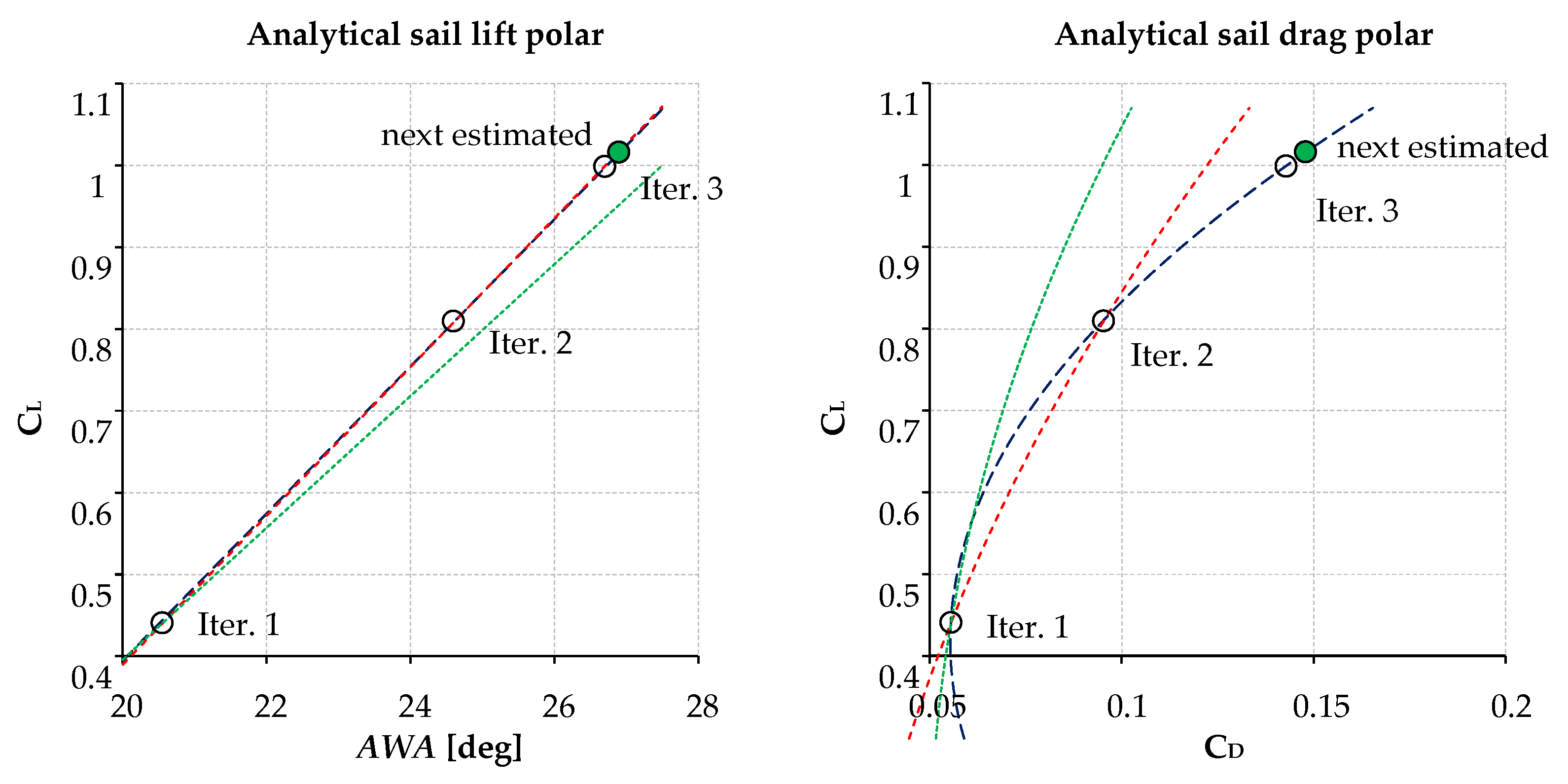
• In the first iteration the sail lift curve slope ${\left(\frac{\partial C_L}{\partial \alpha }\right)}_S$ and the induced drag factor $e_S$ are estimated from literature as function of sail aspect and taper ratio. The value of zero-lift drag coefficient $C_{D0}{}_S$ is roughly guessed. The sail lift and drag coefficients $C_L{}_S$ and $C_D{}_S$, obtained from the CFD analysis, are used to estimate $C_{L0}{}_S$ from Equation (25) and $k_S$ from Equation (26).
• In the second iteration the additional CFD solution is used to complete the analytical lift curve formulation adjusting the values of the lift curve slope ${\left(\frac{\partial C_L}{\partial \alpha }\right)}_S$ and zero-incidence lift coefficient $C_{L0}{}_S$. The parameters updated in the polar curve are $C_{D0}{}_S$ and $k_S$ while the value of $e_S$ is still guessed.
• In the third iteration the analytical drag polar formulation is completed with the computation of the induced drag factor $e_S$ which is last unknown parameter. The lift curve is updated connecting a quadratic formulation to the previous computed linear part.
• In all the following iterations the sailing condition estimation are performed modelling the polars regions under investigation updating both curves by a generic quadratic formulation using the closest three solutions.

Figure 12 reports, for a typical A-Class sail plan, an example of the evolution of the sail polars computation during the progress of the first three iterations and the estimation of the values to be used for the computation of the sailing conditions in the fourth iteration (green circles). If the sail aerodynamic conditions fall in the linear region of the lift curve three iterations are in general sufficient to converge. If not, the reported analytical polars formulation are no more valid. The quadratic formulations, with which the non-linear sail aerodynamics is modelled in the following iterations, simply constitute interpolating curves whose coefficients have no particular physical meaning.

The searching criterion of the aerodynamic coefficients in the inner cycle is driven by an optimization procedure, based on the Nelder–Mead Simplex algorithm [29], whose objective function is the minimisation of the differences between the forces derived from the boat analytical model and from the CFD computation:

$$Obj.Func.=\left|D_{TOT}-F_t{}_{CFD}\right|+\left|F_h-F_h{}_{CFD}\right|$$

(30)

The values of $V$ and $TWA$ that satisfy the equilibrium are used in the next external loop where the sail polars are updated. The iterations continue up to the satisfaction of the equilibrium system in both loops. When the convergence is reached, the boat VMG is computed and produced as output.

It was experienced that the number of RANS computations required to reach a convergence rarely was higher than four or five (if sail is not stalled or, in general, if separations are not too large). Furthermore, a restarting procedure from the previous solution and a progressive reduction of the CFD iterations, was implemented. This strategy showed to be very efficient in boosting the convergence, but its robustness is related to the capability to select starting sailing conditions as realistic as possible. The procedure fails in case of sudden sail separation. To reject such solutions a check if complete stall occurs was implemented.

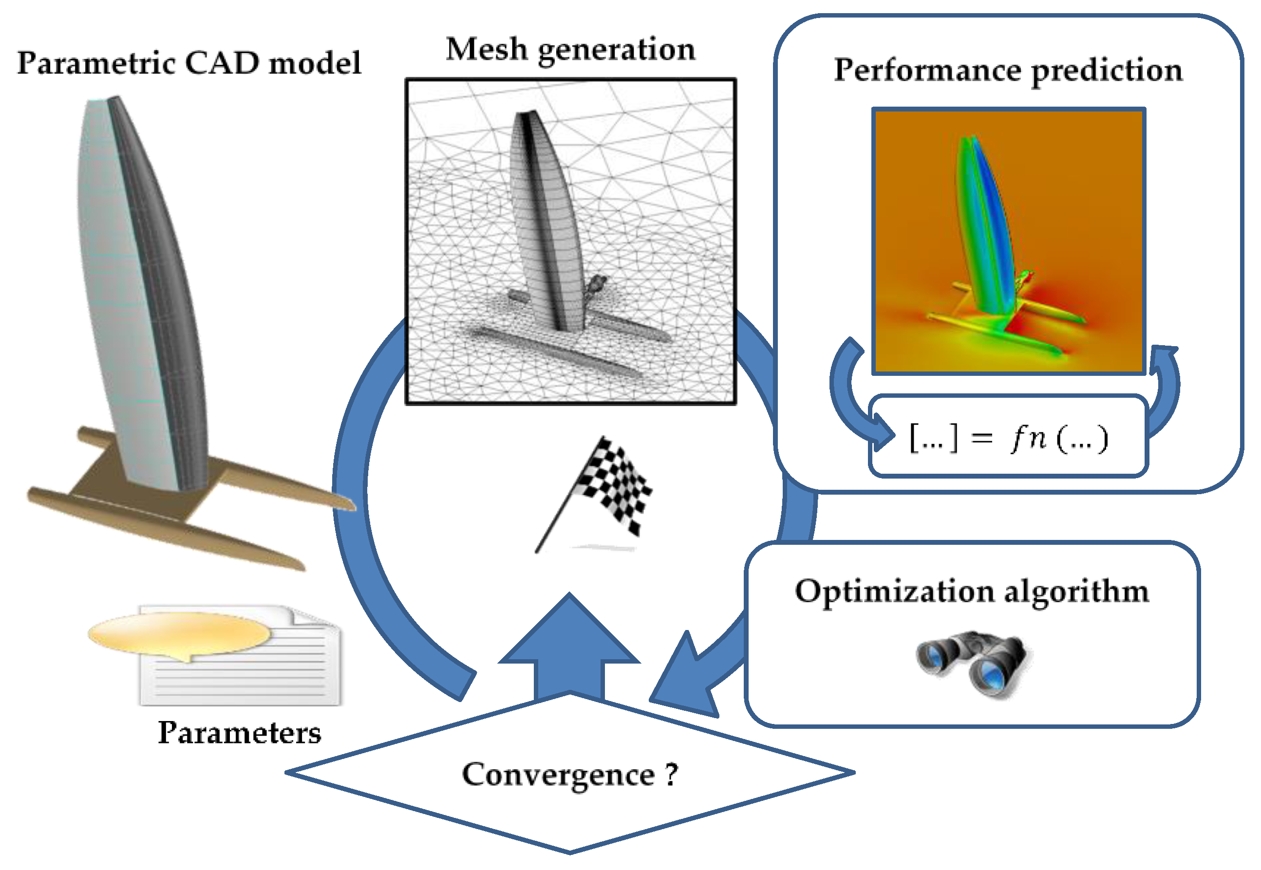
3. Optimization Environment

The above-described performance prediction procedure was integrated in an optimization environment in which the optimal sail plan, trim and appendage configuration is researched. Several approaches are possible to parametrize the geometry. A very efficient method consists in adopting mesh morphing techniques [30]. Such approach has the advantage to operate directly on the numerical domain avoiding the remeshing requirement. The adoption of structured meshes or efficient remeshing algorithms, however, might allow to develop procedures with computational efforts comparable to mesh morphing strategies. The method here presented integrates, in an automatic process, the sail parametric CAD model, the computational domain generation, the RANS analysis and the VPP model.

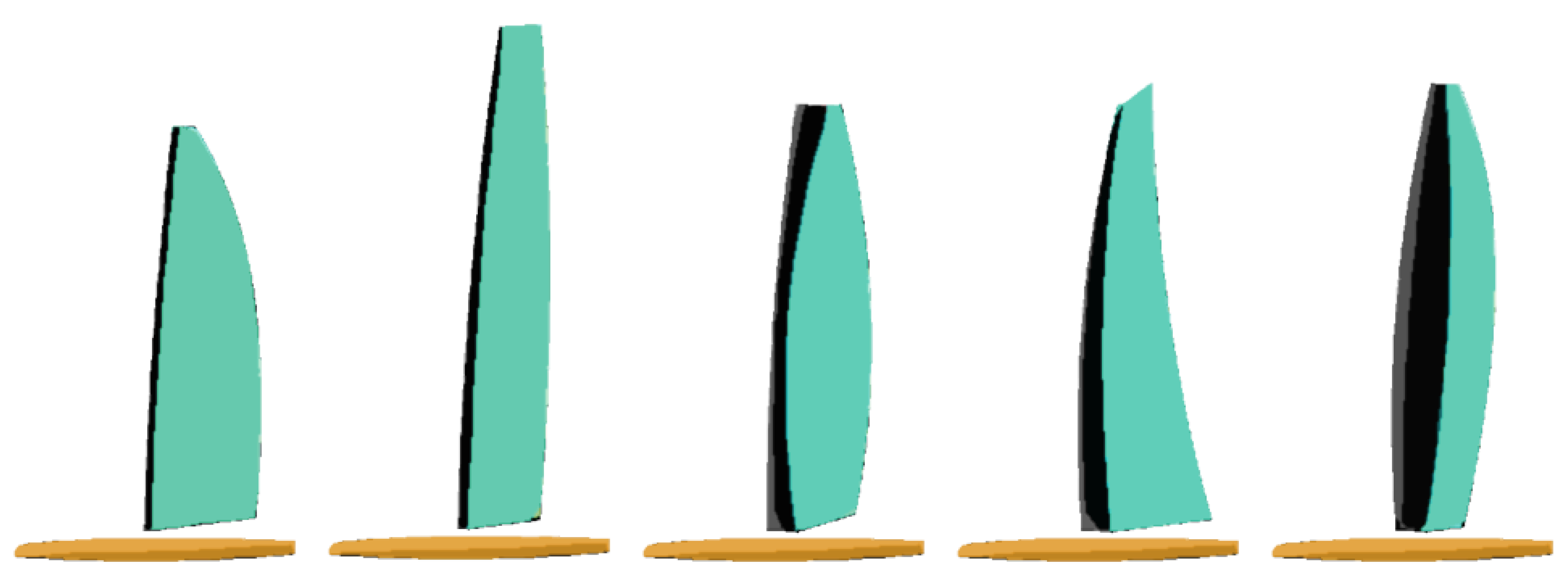
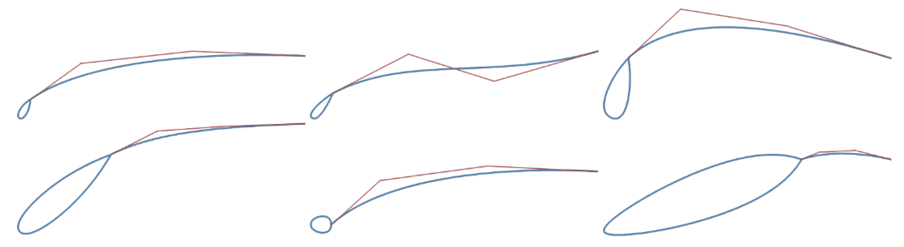
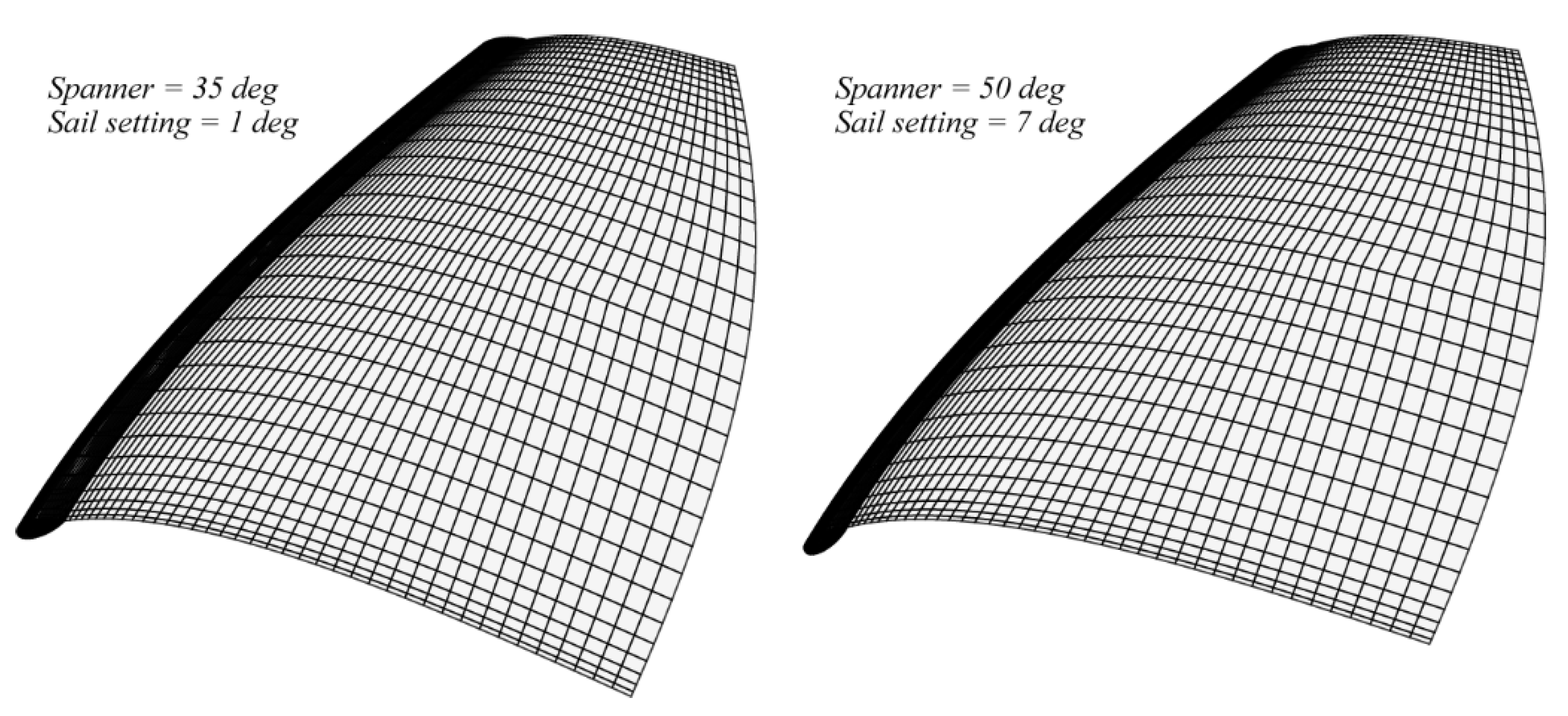
3.1. Sail Parametric Geometric Module

The selected strategy to parametrise the computational domain is based on the update of a parametric CAD model and in the regeneration of the CFD mesh. The software used is the Open-Source FreeCAD (www.freecadweb.org accessed on 1 April 2021) tool, a general-purpose parametric 3D CAD modeller [31]. The software can also be used as a library by other programs. The geometry generation and its exportation are managed by a Python script (Figure 13).

The topology of the sail plan consists in a single mast/mainsail configuration. The CAD parameters were selected with the aim to investigate the largest possible range of geometries. Traditional sail plans, wing masts or wing sails with a small portion of flexible sail can be generated. The model is built by a loft surface through a foot, an intermediate arbitrarily positioned and a head curve that are used as control sections. The luff curve is used as guide. In a similar manner, the mast is generated from three geometries at the same stations. The planform is controlled by reference surface, aspect ratio, taper ratio and by other parameters that give the possibility to investigate a wide range of shape. The examples in Figure 14 give the sense on the flexibility of the parametric model.

The sail sections are generated by cubic Bezier curves. The first point of the control polygon is connected to the mast luff, the last one coincides with the leech of the sail. The four coordinates of the two intermediate control points are parameters of the geometry (red polylines in Figure 15). The mast sections are generated by spline curves controlled by three parameters. The spanner angle (angle between the mast chord and the boat symmetry plane) is a setting parameter. The input reference surface area is kept unchanged. After the geometry creation, the final sail area is measured and the loft surface cut in order to restore the required value. The procedure is linked to the sail CFD analysis module. Two versions of the fluid dynamic computation were setup: one based on commercial software and one based on an Open-Source solver.

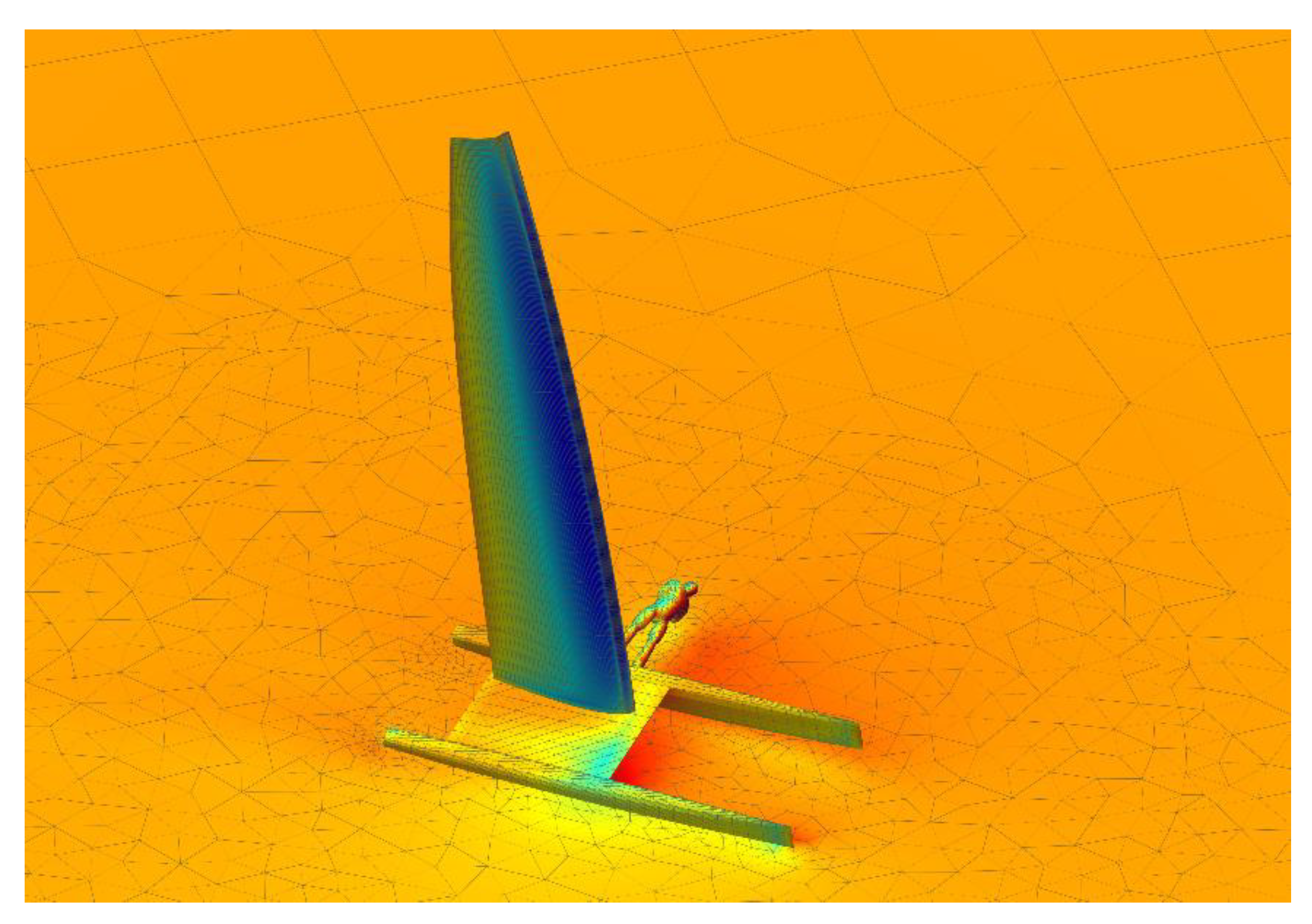
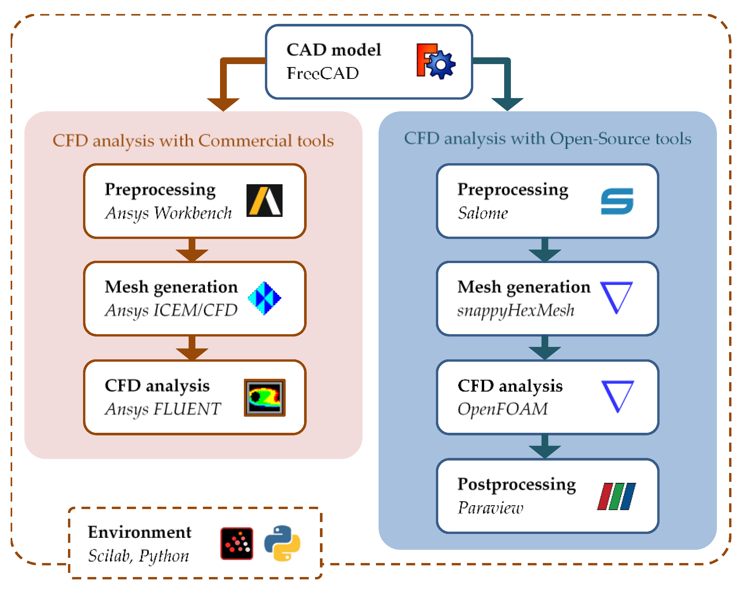
3.2. Sail CFD Analysis Module Implemented Adopting Commercial Software

A well consolidated mesh update procedure [32], widely applied to several aerodynamic optimization problems, was implemented. It is based on an automatic generation of a structured hexahedral multiblock mesh using ANSYS ICEM/CFD and in the run of the analysis using the CFD ANSYS Fluent solver. Due to the complexity of the geometry (all of the boat, included the helmsman, is modelled) a mixed strategy, in the mesh generation, was adopted. The domain was divided in several regions with common boundaries and each region was meshed applying the more appropriate strategy. A structured CH grid topology was created in a limited volume around the sail and dimensioned to envelope the full range of possible geometries. An unstructured hybrid prism/tetra mesh was generated around the boat in the volume between the sail structured mesh and the water plane. The sail/boat mesh assembly is contained in a box, four boat lengths large and tall, in which another hybrid prism/tetra mesh portion was generated. The remaining volume was meshed with hexahedral cells growing toward the top with a progression aimed to better model the inflow air boundary layer. The full domain is 10 boat lengths wide and is extended 10 boat lengths upstream and downstream the model. The several elements of the mesh are connected by zonal interface boundaries in which a simple “flow-through” condition between the non-conformal zones is imposed. The first image of Figure 16 shows the assembly of the parts with the interfaces in evidence. The other two images detail the structured grid around the sail which is the only part of the mesh subjected to update every optimization iteration.

Figure 17 reports the final assembly of the mesh. The total dimension is around half millions of cells. This value was selected after a mesh sensitivity analysis. It was evaluated as a reasonable compromise between accuracy and computational costs being the mesh to be adopted for an optimization procedure in which is more important the difference between candidates than the absolute accuracy of the analysis.

The numerical analysis consists in a steady fully turbulent RANS computation. The extracted solutions are the sail heeling and thrust forces, in upwind sailing conditions, together with the resultant aerodynamic centre of pressure. The two-equation $k-\omega$ SST (Shear Stress Transport) turbulence model of Menter [33] was used. Wall Functions were applied to model the wall boundary layer. The boat is moving on a local reference frame at the given speed $V$ and direction $TWA$ with respect to the true wind. These values are updated iterating with the analytical boat model in a process that constitutes the VPP module that provides the performance of the boat with the selected geometric configuration. At far field the wind boundary layer velocity profile [34] in the absolute reference frame is imposed. A pressure outlet is imposed at the outlet boundary behind the boat. Figure 18 reports the solution on a typical geometry with 10 knots of true wind speed at 10 m from the water plane. The streamlines evidence the structures of the sail tip and root vortices. The wind boundary layer velocity magnitude is reported by a contour plot on a plane behind the boat.

Sails often exhibits separations in the region of the mast (Figure 19 reports an example of the typical evolution of this phenomenon behind a traditional A-Class rig). Furthermore, they usually perform in high lift conditions when trailing edge separations might also occur. The solver convergence histories could then be affected by unsteadiness or, in general, by irregularities. The simple extraction of the value of the last iteration might provide misleading information. A routine able to filter and to evaluate the quality of the solutions was then developed. It consists in extracting a linearized interpolation of the last portion of the convergence history, in evaluating its slope, the maximum deviation of the solution from it and in extracting a value applying opportune constraints in order to reject unacceptable solutions. Figure 20 reports an example of how this filter works.

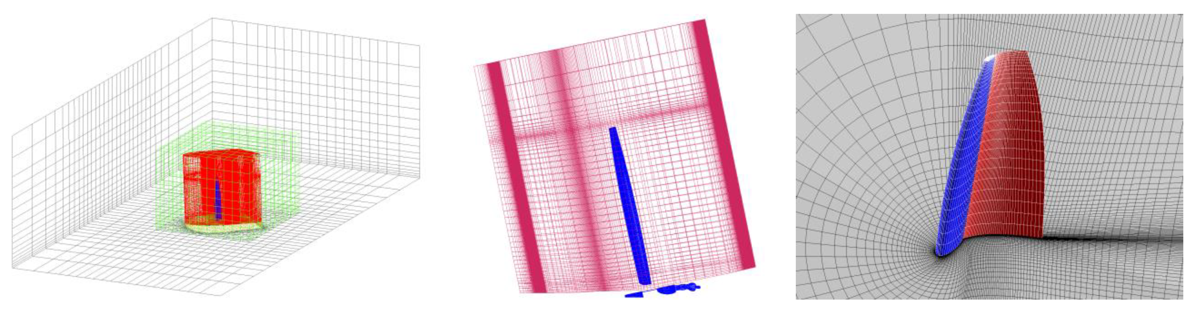
3.3. CFD Analysis Module Based on Open-Source Tools

The CFD analysis module was replicated adopting Open-Source codes. The objective is to make available a tool completely unlinked from commercial software. The workflow of the developed procedure is sketched in Figure 21. The steps of the process are summarized below:

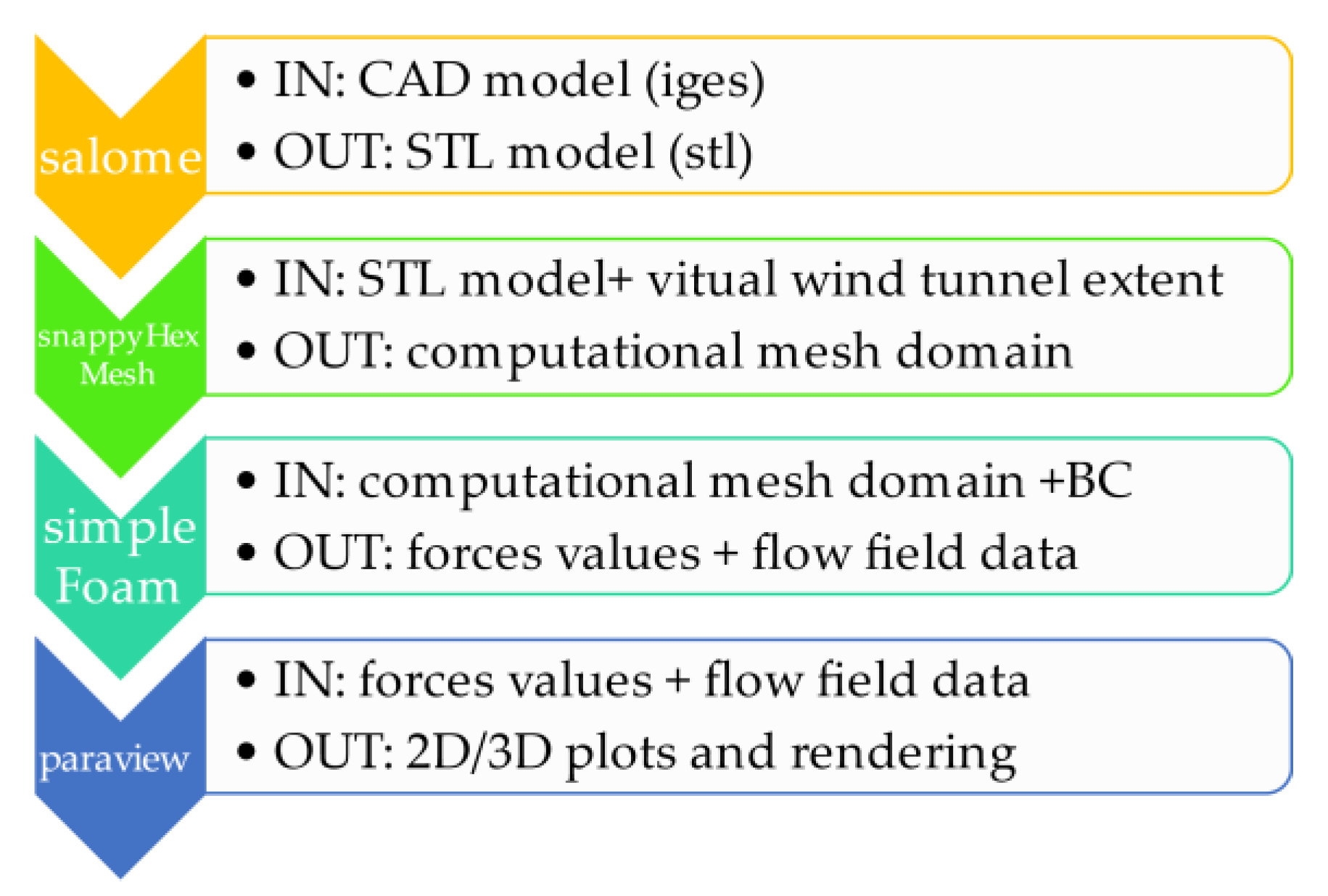
• CAD import and pre-processing;
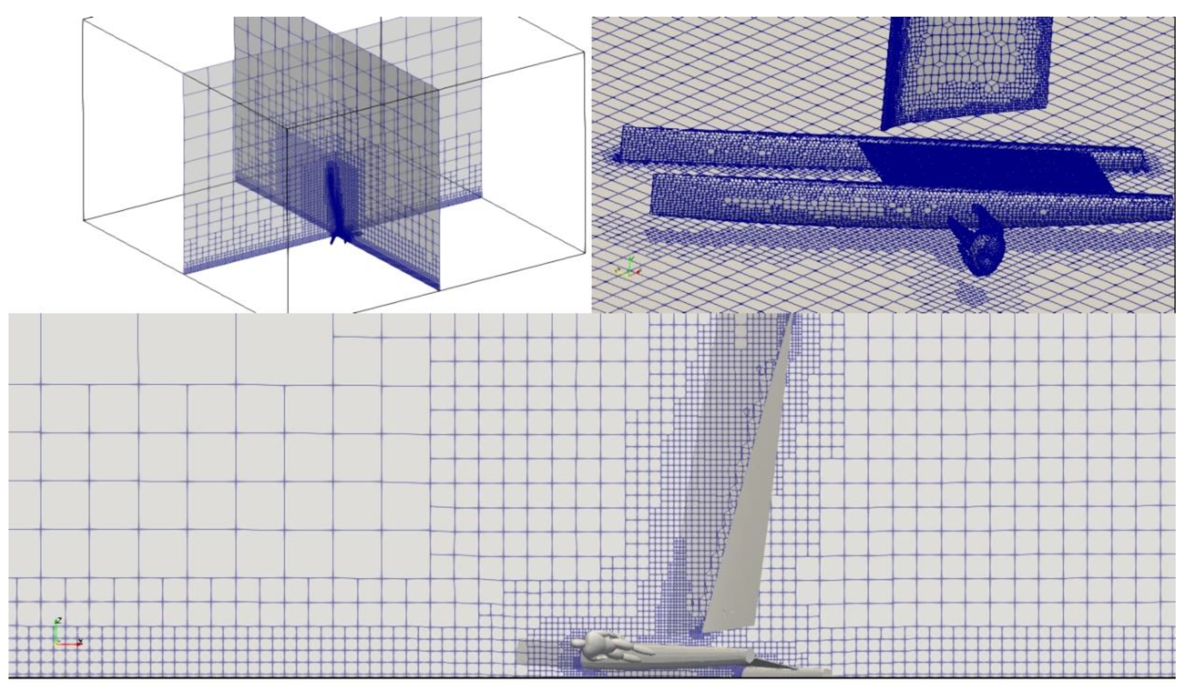
• Geometry meshing;
• Flow field solving;
• Data visualisation and post-processing.

The baseline CAD model contains the boat (hull, platform, mast and sail) and the body of the sailor. The flow solver used is OpenFOAM. The mesh was generated by the mesher SnappyHexMesh with the support of Salome-Mesh, which was used to generate the triangularisation of the surfaces. The domain is built by defining a background mesh that is iteratively refined accordingly to geometry CAD surface intersection and projection (top-down approach). This technique is very flexible and very low demanding with respect to the quality of the geometry CAD surface definition. The typical resulting computational domain and the mesh are showed in Figure 22.

The simpleFoam solver with the $k-\omega$ SST turbulence model was used. The simulations have been conducted in the relative reference frame where the boat is stationary and the wind swirling boundary profile is generated at far field by its components tabulated in a formatted file. Wall functions were adopted to model the boundary layer. From preliminary analyses it was observed the Open-Source CFD configuration to provide a solution that differ in the order of 3–5% with respect to the solutions obtained with the commercial solver Figure 23 reports a typical convergence history of the solutions.

To include the Open-Source based analysis in the optimization environment, the following steps were implemented in an automatic procedure by a set of batch scripts and Python routines:

• Conversion from CAD to STL;
• Mesh generation and CFD configuration update;
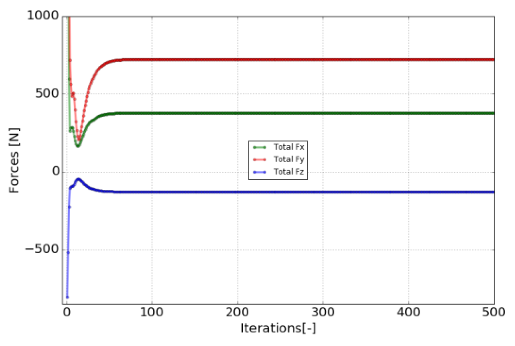
• CFD run and solutions export;
• Post-processing and results extraction.

The obtained procedure is ready to substitute the commercial based one in the optimization environment. Figure 24 lists the software adopted to implement the two CFD analysis modules.

3.4. Implementation of the Optimization Environment

Figure 25 sketches the workflow of the implemented optimization procedure. After the CAD model update the process is guided by a script that loads the new geometry, recomputes the mesh and exports the new grid in the solver format. The CFD configuration is then updated and the VPP module, described in the previous section, executed to provide the performance of the selected configuration. According to the solutions obtained, the optimization algorithm selects a new combination of parameters and the cycle progress until the “Optimum” configuration is identified. All the modules are managed by Scilab routines.

More than 40 parameters can be selected to characterise the boat configuration (airfoil, planform, positions and attitude of appendages as well as the parameters controlling the shape and the trim of the sail rig). Such a wide range of potential design variables gives great flexibility in exploring innovative solutions. The optimization environment, furthermore, provides the designer a powerful tool that supports the exploration of their limits.

4. Test of the Analysis Modules

The analysis modules were tested on a simplified optimization problem. It consisted in defining a DOE matrix, using two design variables, and in the definition of a response surface on which to search the optimum. The test has the double objective to find out potential criticisms of the CFD workflows and to compare the performance of the commercial and the Open-Source based analysis procedures. The optimization problem consisted in finding the optimum sail setting of an A-Class traditional rig at a fixed boat speed $V=10$ knots, a true wind angle $TWA=45$ deg and a true wind speed $TWS=10$ knots. The variables were the mast spanner angle and the sail setting intended as the angle between the sail chord at the base and the symmetry plane of the boat. It was decided a range of variation for the spanner from 35 to 50 degree with a step of 5 deg. The range of variation of the sail setting angle was from 1 to 7 degree with a step of 2 deg. The DOE table was then populated with 16 solutions. Figure 26 reports the geometries of two design candidates belonging to two extremes of the variables design space.

The target of the optimization was the maximisation of the sail thrust force. The objective function to maximize was defined as follows:

$$Obj.Func.=F_t=F_Y\mathit{sin}TWA-F_X\mathit{cos}TWA$$

(31)

where the input forces are referred to a frame aligned to the true wind speed direction.

The optimum sailing condition of classic catamarans is with the upwind hull in flying condition just outside the water. This is also the conditions at which almost the maximum righting moment is generated. In equilibrium conditions, the heeling moment must be equal to the righting moment. Assuming the helmsman is positioned at the trapeze, having a weight of 90 kg and an arm slightly higher than 3 m, the maximum allowable righting moment, including the contribution of the boat weight ($M_h{}_{max}$), is around 3500 Nm. This value was implemented as an optimization constraint:

$$M_Y\mathit{sin}TWA-M_X\mathit{cos}TWA\le M_h{}_{max}$$

(32)

Figure 27 compares the response surfaces computed with the solutions obtained by the two solvers. A second-degree polynomial formulation was sufficient to approximate the computed CFD solutions generating a residual error always below 0.3%.

The colours of the response surfaces are associated to the value of the heeling moment. The black curves on the surfaces are the $M_h{}_{max}$ isolines at 3500 Nm. The optimum solution has then to be searched along these curves. The green points indicate the positions of the optima solutions found with the two methods. The optimum found using ANSYS Fluent is located on the boundary of the variables space since the isocurve do not have a maximum within his domain. The maximum found with the OpenFOAM based analysis procedure is close to the middle of the spanner range. The

Table 2. Optima rig setting solutions.

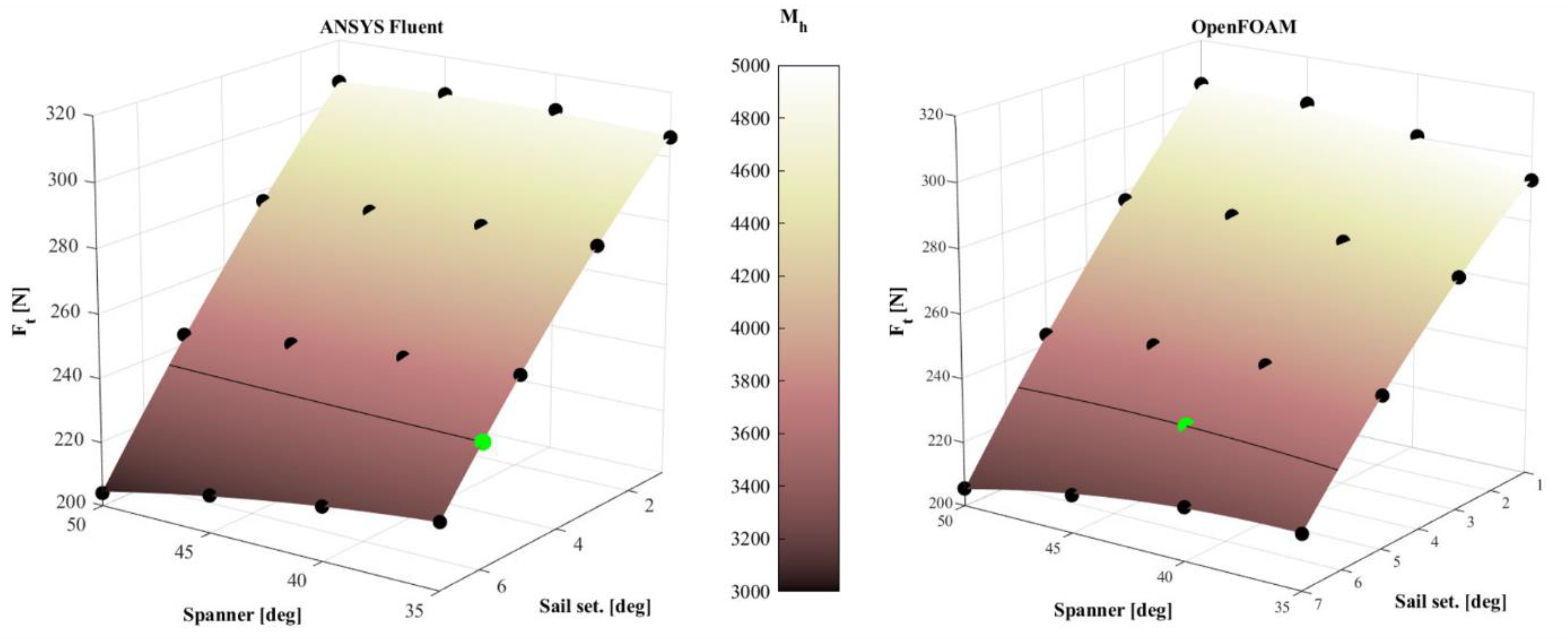
	ANSYS Fluent	OpenFOAM
Spanner	35 deg	41.7 deg
Sail setting	5.9 deg	6 deg
Thrust force	238.2 N	232.5 N

reports the two optima solutions.

The thrust force estimated by the Open-Source based analysis procedures has a difference in the order of 2.4% with respect to the solution obtained by the commercial based analysis procedure. Both estimated almost the same optimum sail setting while larger differences are observed concerning the spanner setting. This variable, in fact, was shown to cause the generation of an isoline on which to search for the optimum almost horizontal in a wide range of the variable values. As a consequence, small differences in the solutions of the two solvers led to the identification of very different optima that, nevertheless, generated very similar performances. In other words, the spanner angle showed to have a moderate impact on the objective function in a wide range of the variable space.

Figure 28 compares the pressure distribution obtained by the two solvers for the configuration with the spanner angle equal to 50 degrees and the sail setting at five degrees. The two solutions are very similar, confirming the quality of the Open-Source solution in comparison to the commercial one.

The ANSYS Fluent based analysis procedure ran on a workstation equipped with 20 cores (2 processors Intel Xeon E5-2680 2.8 GHz with 10 cores each). The complete convergence was reached, for each design points, with 200 iterations in less than ten minutes. The OpenFOAM based procedure ran on HPC nodes equipped with Intel Xeon 2670 v2 2.5 GHz. A single run required 15 min with 20 cores to complete the CAD setting, mesh generation, computation and solution extraction process. The computational costs of the two methods can then be in general considered comparable. As concluding remarks, it can be stated that the Open-Source based analysis module can be considered a valid candidate to replace the commercial based procedure.

5. Conclusions

A numerical optimization environment for a catamaran’s sail plan and appendages, that couples a VPP based on analytical models and on a sail RANS computation, was developed. Two versions of the CFD analysis module were implemented and compared: one based on commercial software and one fully based on Open-Source tools. The procedures that manage the several modules were written using the Scilab computing environment. The geometric parametric module was implemented by Python scripts used to drive the Open-Source FreeCAD software to generate the CAD model. The analytical formulations, used to model the hull and the appendages forces, were implemented in a form of independent functions and coupled to the CFD solutions of the sail to solve the equilibrium system of equations of the boat in an iterative procedure. This procedure constitutes the VPP module that estimates the performance of the selected configuration in terms of boat VMG in upwind sailing conditions. The analysis is performed, in the procedure based on commercial software, using ANSYS ICEM/CFD to generate the mesh and ANSYS Fluent to provide the aerodynamic solution. In the Open-Source based analysis, the tools adopted were Salome-Mesh for pre-processing, SnappyHexMesh for the mesh generation, OpenFOAM for the CFD solution and Pareview for the post-processing. The performance of the two analysis modules were compared applying them on a simple test case: the optimization of the setting of the sail rig of an A-Class catamaran defined by two variables. A DOE approach was adopted, and a response surface generated on the solutions obtained with the two procedures. The objective function was the maximization of the sail thrust force with the constraint of a fixed heeling moment.

The two methods generated relatively similar optima solutions (with a difference in the objective function in the order of 2%). Except for cases where significant separation was present (close to the maximum lift), OpenFOAM provided, in general, solutions whose differences were lower than 5% with respect to the forces obtained with ANSYS Fluent. The difference of the thrust force of the two optima solutions was in the order of 2.4%. Considering that an optimum solution is expected to have no separations (or at least limited separated regions), it thus can be stated that OpenFOAM is a valid candidate to replace ANSYS Fluent in the optimization procedure. This assumption is also valid evaluating the computational requirements of the two solvers. Both codes completed an analysis of a case with attached flow in less than 15 min using 20 cpu.

References

- Fossati, F. Aero-Hydrodynamics and the Performance of Sailing Yachts: The Science behind Sailing Yachts and Their Design; A&C Black: London, UK, 2009. [Google Scholar]
- Lasher, W. The determination of aerodynamic forces on sails—Challenges and status. In Atmospheric Turbulence, Meteorological Modelingand Aerodynamics; Nova Science Publishers: Hauppauge, NY, USA, 2011; pp. 487–504. [Google Scholar]
- Day, A.H.; Cameron, P.; Dai, S. Hydrodynamic Testing of a High Performance Skiff at Model and Full Scale. J. Sail. Technol. 2019, 4, 17–44. [Google Scholar] [CrossRef]
- Graf, K.; Boehm, C. Coupling of ranse-CFD with VPP methods: From the numerical tank to virtual boat testing. In Proceedings of the 2nd International Conference on Innovation in High Performance Sailing Yachts, Lorient, France, 30 June–1 July 2010. [Google Scholar]
- Lasher, W.C.; Richards, P.J. Validation of Reynolds-Averaged Navier-Stokes Simulations for International America’s Cup Class Spinnaker Force Coefficients in an Atmospheric Boundary Layer. J. Ship Res. 2007, 51, 22–38. [Google Scholar] [CrossRef]
- Peart, T.; Aubin, N.; Nava, S.; Cater, J.; Norris, S. Multi-Fidelity Surrogate Models for VPP Aerodynamic Input Data. J. Sail. Technol. 2021, 6, 21–43. [Google Scholar] [CrossRef]
- Fossati, F.; Muggiasca, S.; Viola, I.M. An investigation of aerodynamic force modelling for IMS rule using wind tunnel techniques. In Proceedings of the 19th International HISWA Symposium on Yacht Design and Yacht Construction, Amsterdam, The Netherlands, 13–14 November 2006. [Google Scholar]
- Graf, K.; Freiheit, O.; Schlockermann, P.; Mense, J.C. VPP-Driven Sail and Foil Trim Optimization for the Olympic NACRA 17 Foiling Catamaran. J. Sail. Technol. 2020, 5, 61–81. [Google Scholar] [CrossRef]
- Findlay, M.W.; Turnock, S.R. Investigation of the effects of hydrofoil set-up on the performance of an international moth dinghy using a dynamic VPP. In Proceedings of the Innovation in High Performance Sailing Yachts, Lorient, France, 29–30 May 2008. [Google Scholar]
- Bagué, A.; Degroote, J.; Demeester, T.; Lataire, E. Dynamic Stability Analysis of a Hydrofoiling Sailing Boat using CFD. J. Sail. Technol. 2021, 6, 58–72. [Google Scholar] [CrossRef]
- Cella, U.; Salvadore, F.; Ponzini, R. Coupled Sail and Appendage Design Method for Multihull Based on Numerical Optimisation; EU SHAPE Project Final Report; PRACE: Bruxelles, Belgium, 2016. [Google Scholar]
- Gomez, C.; Bunks, C.; Chancelier, J.P.; Delebecque, F.; Goursat, M.; Nikoukhah, R.; Steer, S. Engineering and Scientific Computing with Scilab; Gomez, C., Ed.; Birkhäuser: Basel, Switzerland, 1999. [Google Scholar]
- Gerritsma, J.; Onnink, R.; Versluis, A. Geometry, resistance and stability of the Delft systematic yacht hull series. Int. Shipbuild. Prog. 1981, 28, 276–297. [Google Scholar] [CrossRef]
- Keuning, L.J.; Katgert, M. A bare hull resistance prediction method derived from the results of The Delft Systematic Yacht Hull Series to higher speeds. In Proceedings of the Innovation in High Performance Sailing Yachts, Lorient, France, 29–30 May 2008. [Google Scholar]
- Kerdraon, P.; Horel, B.; Bot, P.; Letourneur, A.; le Touzé, D. High Froude Number Experimental Investigation of the 2 DOF Behavior of a Multihull Float in Head Waves. J. Sail. Technol. 2021, 6, 1–20. [Google Scholar] [CrossRef]
- Molland, A.F.; Turnock, S.R.; Hudson, D.A. Ship Resistance and Propulsion; Cambridge University Press: New York, NY, USA, 2011. [Google Scholar]
- de Luca, F.; Mancini, S.; Miranda, S.; Pensa, C. An Extended Verification and Validation Study of CFD Simulations for Planing Hulls. J. Ship Res. 2016, 60, 101–118. [Google Scholar] [CrossRef]
- Zou, L.; Larsson, L. CFD Verification and Validation in Practice—A Study Based on Resistance Submissions to the Gothenburg 2010 Workshop on Numerical Ship Hydrodynamics. In Proceedings of the 30th Symposium on Naval Hydrodynamics, Hobart, Australia, 2–7 November 2014. [Google Scholar]
- Insel, M.; Molland, A. An Investigation into the Resistance Components of High Speed Displacement Catamarans; RINA: Genoa, Italy, 1992. [Google Scholar]
- Hoerner, S.F. Fluid-Dynamic Drag; Hoerner Fluid Dynamics: Brick Town, NJ, USA, 1965. [Google Scholar]
- ITTC. Resistance Uncertainty Analysis, Example for Resistance Test. In Proceedings of the ITTC International Towing Tank Conference, Recommended Procedures, Venice, Italy, 14–16 January 2002. [Google Scholar]
- Losito, V. Fondamenti di Aeronautica Generale; Accademia Aeronautica Pozzuoli: Pozzuoli, Italy, 1991. [Google Scholar]
- Roskam, J. Airplane Aerodynamics and Performance; DARcorporation: Lawrence, KS, USA, 1997. [Google Scholar]
- Drela, M. XFoil—An Analysis and Design System for Low Reynolds Number Airfoils. In Low Reynolds Number Aerodynamics. Lecture Notes in Engineering; Springer: Berlin/Heidelberg, Germany, 1989; Volume 54, pp. 1–12. [Google Scholar]
- Abbott, A.H.; von Doenhoff, A.E. Theory of Wing Sections; Dover Publications: Mineola, NY, USA, 1959. [Google Scholar]
- Perkins, C.D.; Hage, R.E. Airplane Performance Stability and Control; John Wiley & Sons: New York, NY, USA, 1949. [Google Scholar]
- Larsson, L.; Eliasson, R. Principle of Sailing Yacht Design; Adlard Coles Nautical: London, UK, 1997. [Google Scholar]
- Claughton, A.; Wellicome, J.; Shenoi, A. Sailing Yacht Design: Theory; Longman: London, UK, 1998. [Google Scholar]
- Nelder, J.A.; Mead, R. A Simplex Method for Function Minimization. Comput. J. 1965, 7, 308–313. [Google Scholar] [CrossRef]
- Biancolini, M.E.; Viola, I.M.; Riotte, M. Sails trim optimisation using CFD and RBF mesh morphing. Comput. Fluids 2014, 93, 46–60. [Google Scholar] [CrossRef]
- Cella, U.; Cucinotta, F.; Sfravara, F. Sail Plan Parametric CAD Model for an A–Class Catamaran Numerical Optimization Procedure Using Open Source Tools. In Advances on Mechanics, Design Engineering and Manufacturing; Lecture Notes Series in Mechanical Engineering; Springer: Cham, Switzerland, 2016. [Google Scholar]
- Cella, U.; Romano, D.G. Winglets design and assessment of optimization algorithms. In Proceedings of the CAE Technologies International Conference, Bergamo, Italy, 1–2 October 2009. [Google Scholar]
- Menter, F.R. Two-equation eddy-viscosity turbulence models for engineering applications. AIAA J. 1994, 32, 1598–1605. [Google Scholar] [CrossRef]
- Musker, A.J. Explicit Expression for the Smooth Wall Velocity Distribution in a Turbulent Boundary Layer. AIAA J. 1979, 17, 655–657. [Google Scholar] [CrossRef]