Artificial Intelligence Application on Sediment Transport

Abstract

When erosion occurs, sand beaches cannot maintain sufficient sand width, foreshore slopes become steeper due to frequent erosion effects, and beaches are trapped in a vicious cycle of vulnerability due to incident waves. Accordingly, beach nourishment can be used as a countermeasure to simultaneously minimize environmental impacts. However, beach nourishment is not a permanent solution and requires periodic renourishment after several years. To address this problem, minimizing the period of renourishment is an economical alternative. In the present study, using the Tuvaluan coast with its cross-sectional gravel nourishment site, four different test cases were selected for the hydraulic model experiment aimed at discovering an effective nourishment strategy to determine effective alternative methods. Numerical simulations were performed to reproduce gravel nourishment; however, none of these models simultaneously simulated the sediment transport of gravel and sand. Thus, an artificial neural network, a deep learning model, was developed using hydraulic model experiments as training datasets to analyze the possibility of simultaneously accomplishing the sediment transport of sand and gravel and supplement the shortcomings of the numerical models.

1. Introduction

Coastal erosion has natural causes, such as sea-level rise and wave energy increase. However, it can be accelerated by changes in the natural environment due to various artificial structures installed on the coast. Coastal zones are significant for society’s development, but they are particularly vulnerable to the impacts of nature and humans and are physically very unstable. Erosion and the associated loss of land are the most evident signs of this instability. Negative shoreline trends cause secondary effects on society, particularly threats to human settlements. However, most natural sandy beaches cannot prevent extreme waves and storm surges from causing beach erosion. This erosion happens due to steep aggressive storm waves and accretion that build ups on the beach with less steep, non-aggressive waves. Thus, coastal structures can be used in erosive beaches.

Coastal structures are generally built at locations where beach erosion causes severe problems. The decision to build a coastal structure should be based on a thorough analysis of past shoreline developments and future estimated events. Accordingly, the physical processes that cause erosion should be properly identified. There are two main categories of coastal protection methods: hard and soft. Hard methods include seawalls, revetments, or jetties, which intercept and dissipate wave energy, currents and associated sand transport. However, these hard structures may enhance erosion in such areas and may collapse if improperly designed, which results in high construction and maintenance costs. By contrast, soft methods aim to dissipate wave energy using natural coastal processes. In this way, coastal defense works in accordance with the natural means of sediment erosion, storage, and transport. This method results in a low-maintenance coastal system that can respond to external forcing factors, such as storms and sea-level rise.

The erosion of the world’s coasts has led to the increasingly common use of gravel for coastal protection, beach nourishment, and sand storage to mitigate beach erosion [1]. Beach nourishment, as a soft technique, can be used as a countermeasure for the erosion problem while minimizing environmental impacts. However, like most soft techniques, it is not a permanent solution and requires periodic renourishment after several years. Beach nourishment incorporates a series of beach renourishment over the long-term horizon or the life cycle of an application. This fact poses difficulties in predicting benefits and costs because of uncertain project performance and future markets for necessary inputs, where sand is the most critical input. With the increasing demand for sand, it is difficult to predict the cost of sand in the future [2]. Thus, reducing the period of renourishment is essential, and slowing down erosion through careful planning of the nourishment’s ability to remain for a prolonged period is crucial. Larger grain-sized sand is said to be more resistant to erosion [3], and many beaches around the world, such as the Jinkoji coast in Japan, Marina di Pisa in Italy, Nice beach in France, and Fongafale shore in Tuvalu [4,5,6,7] have proved that the usage of these gravels as a nourishment material lengthens the period of renourishment.

In this study, Fongafale shore in Funafuti, Tuvalu, was selected as the study site. This shore uses gravel nourishment to protect the coast from erosion. As Tuvalu is a Pacific Island nation, locally available coral gravel is procured as a nourishment material, which is the first trial of a user- and eco-friendly coastal conservation measure in Pacific Island nations. The executed gravel beach nourishment can maintain stability under seasonal and extreme wave action conditions. Throughout the study, gravel and sand with varying placement methods were used to determine the erosion tendencies.

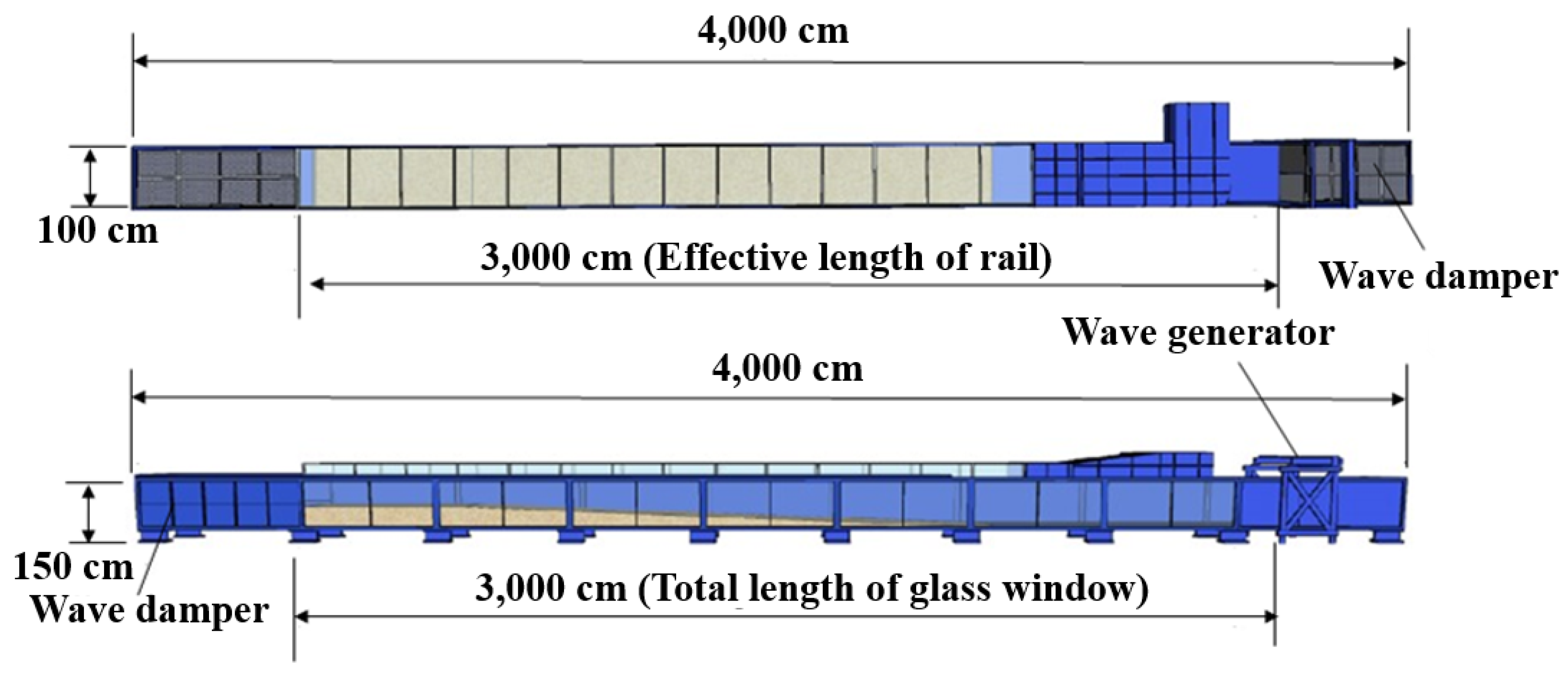
2. Hydraulic Model Experiment

A hydraulic model experiment using a two-dimensional (2D) wave flume was conducted to observe the sediment transport and profile evolution of the different nourishment types. The wave flume used in this experiment was 30 m long, 1 m wide, and 1.8 m high (see Figure 1). The wave maker can generate random and regular waves. Furthermore, it has a wave height gauge attached to the front of the wave paddle to enable reflected wave absorbing control based on the data read by the indicator. In addition, a wave damper, consisting of rubble, Styrofoam, and aluminum pieces, and an absorption filter were installed to minimize the generation of reflected waves.

The Japan International Cooperation Agency (JICA) conducted a gravel nourishment project [8] at the Tuvaluan beach (Figure 2). The typical cross section of the gravel-nourished Tuvaluan coast in the Fongafale shore was used as an initial profile for the hydraulic model experiment, and a geometric scale of 1/25 was used. The initial profile had a berm slope of 1:3.5 and a beach slope of 1:11. Two different still water levels (SWLs) (6 and 8 cm above the mean sea level (MSL), i.e., highest high water level (HHWL) (+1.42 m from MSL) and ground level (+1.92 m from MSL)), were used throughout the experiment. Beach nourishment can help mitigate the erosion process. However, a single nourishment process is not a long-term solution. Erosion will continue to wear away the nourished sand until renourishment is required. Accordingly, the aim of this study was to determine the erosion tendency when using different grain sizes with varying placement methods.

2.1. Experimental Setup

Most of the experimental parameters were considered based on the actual conditions of the Fongafale shore in Tuvalu. From the field study, it was observed that the Tuvaluan coast is a low-wave energy coast [8], where erosion is accelerated by storm waves. The aim of the experiment was to examine how gravel nourishment would react to large external forces, such as Tropical Cyclone Ula which impacted the beach and caused severe damage to the Tuvaluan coast in 2016, and which morphological changes would occur in these situations. Various placement methods were also considered to determine economical methods by prolonging the renourishment period without damaging the aesthetic view. Cyclone Ula (Figure 3) severely impacted the nourished beach. Therefore, the incident wave characteristics of Cyclone Ula were selected as wave characteristics used in the experiment. Froude-scaling principles should be considered to intercompare the observations from differently sized wave flumes [9]. Applying Froude-scaling, whereby the scale considered significant wave height as 5.2 cm, and a period of 1.1 s (based on prototype of H_s = 1.33 m, and T_s = 5.5 s shown in Figure 3) was used for a 2 h duration. The reason for the experiment ending after two hours for each case was that the profile reached an equilibrium state afterward. The gravel covering the surface at the Fongafale shore had a particle diameter of 8–15 cm, and at the bottom of this thick gravel was gravel smaller than the surface, around 2–6 cm. Although scaling down the sand and grain size without the scale effect is usually difficult, the grain sizes (D₅₀) of sand and gravel used in the experiment were chosen as 0.1 and 5.0 mm.

Four test cases using two SWLs in each case in the wave flume—one with HHWL (SWLs 1 and 6 cm above the MSL) and one with the ground level (SWLs 2 and 8 cm above the MSL)—were used to examine the damage of each test (see

Table 1. Four test cases with different sea levels.

Trial	Condition	Wave Characteristics	Sea Level
Case 1-1	Sand Only	Hs = 5.2 m Ts = 1.1 s	SWL 1
Case 1-2			SWL 2
Case 2-1	Gravel Only		SWL 1
Case 2-2			SWL 2
Case 3-1	Sand (Top) + Gravel (Bottom)		SWL 1
Case 3-2			SWL 2
Case 4-1	Sand (Left) + Gravel (Right)		SWL 1
Case 4-2			SWL 2

). Sand and gravel with different placements were selected as design options and were used to plan an effective nourishment strategy. A large grain-size nourishment is more resistant to erosion. However, to achieve similitude, mean diameters similar to those of local prototype gravels were chosen. Therefore, four types of nourishments, with different mean gravel diameters, were used for the experiments.

The initial profiles for each of the four test cases are shown in Figure 4. The experiments were performed for four test cases with the same wave conditions and irregular waves. The spectrum of the irregular wave used in the experiment was a modified Bretschneider–Mitsuyasu (Equations (1) and (2)), which was proposed by Goda for the frequency spectrum of wind waves. For each test case, the profile was measured every 30 min and stopped at 120 min. The total irregular-wave energy E_I was computed using Equation (2), where H_s and T_s represent the significant wave height and period, respectively.

$$S\left(f\right)=0.205 H_s^2{T}_s^{-4}{f}^{-5}\exp \left(-\frac{0.75}{{\left(T_{s}f\right)}^4}\right)$$

(1)

$$E_I=\rho g{\int }_0^{+\infty }0.205 H_s^2{x}^{-5}{e}^{-0.75x^{-4}}dx=0.068\rho g{H}_s^2$$

(2)

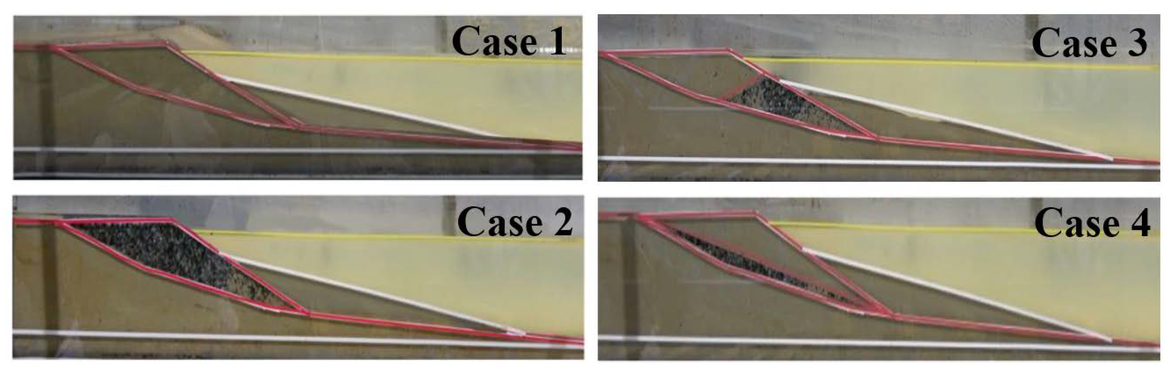
2.2. Hydraulic Model Test Cases

Figure 5 shows an overview of the initial profile of test cases 1 to 4. Case 1 included a berm slope of 1:11 and a foreshore slope of 1:3.5, which corresponded to the sand berm and sand beach without gravel on the berm (see Figure 5). Case 1 was conducted to examine how the other test cases would differ from the one that only used sand for the nourishment.

For test case 2, the initial berm profile was rebuilt on the initial profile for case 1, and the berm was replaced with gravel. D₅₀ of 5 mm of the gravel used in the test was replaced on the sand berm from case 1. This profile was the same as the profile that JICA built on the Tuvaluan coast gravel nourishment area. The idea of this profile was to compare with case 1 and to examine how to effectively decrease or protect against erosion from storm waves.

Gravel nourishment can spoil the aesthetic view and adversely affect natural beaches. Therefore, using only half the amount of gravel used in test case 2, the buried gravel layer was applied in case 3 to reduce the extent of berm erosion without spoiling the shore aesthetics. The gravel layer was first placed on the berm, and sand was placed on top of the layer.

The final test case, test case 4, had the concept of using the same amount of gravel in test case 3, but the building sill type consisted of gravel on the berm covered with sand. After rebuilding the berm sill, a mixture of sand and water was poured into the gravel sill to cover the gravel and fill the voids. All four test cases, with each SWL, were tested for 120 min and the same initial profile was rebuilt after the SWL 1.

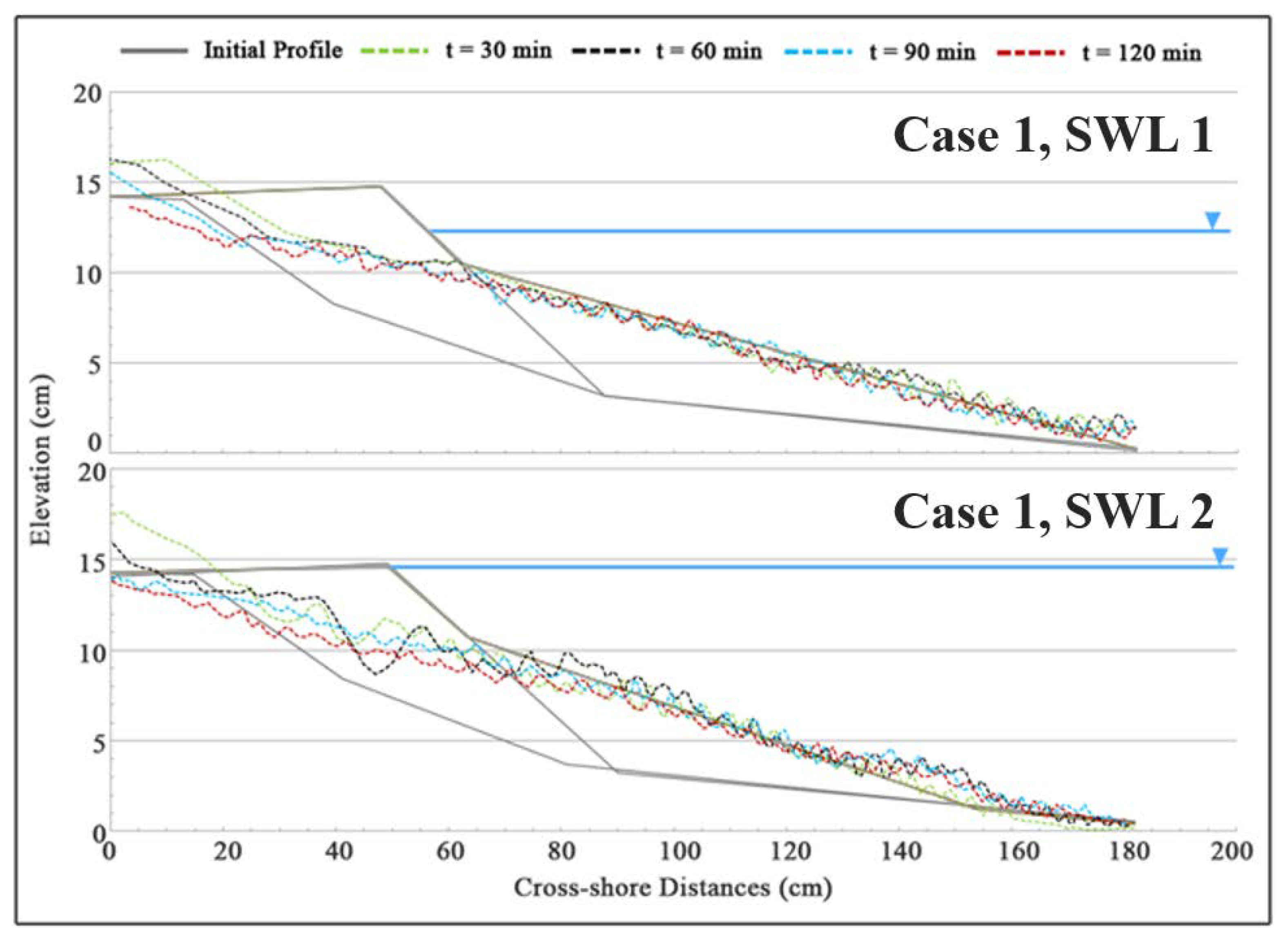
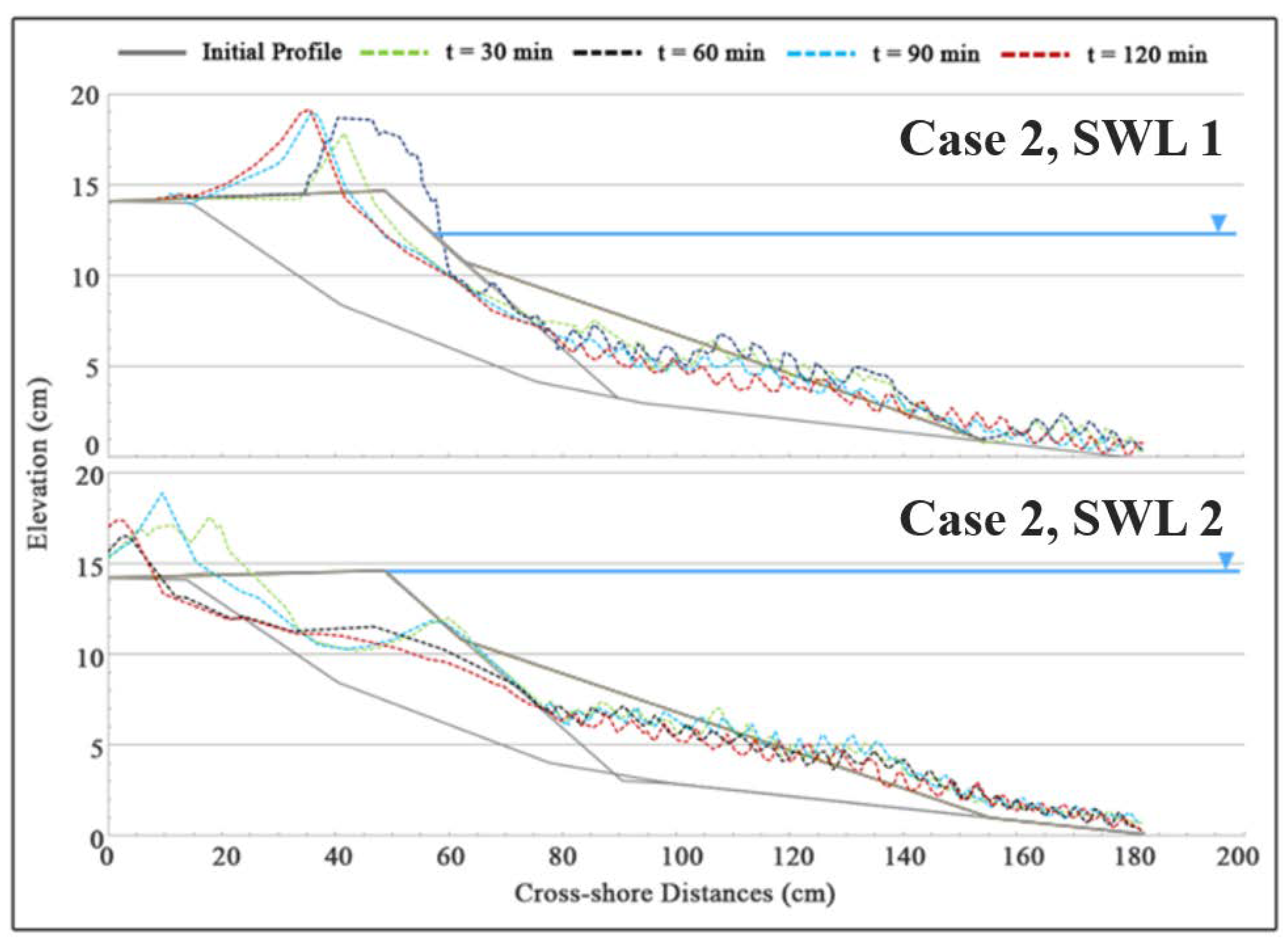
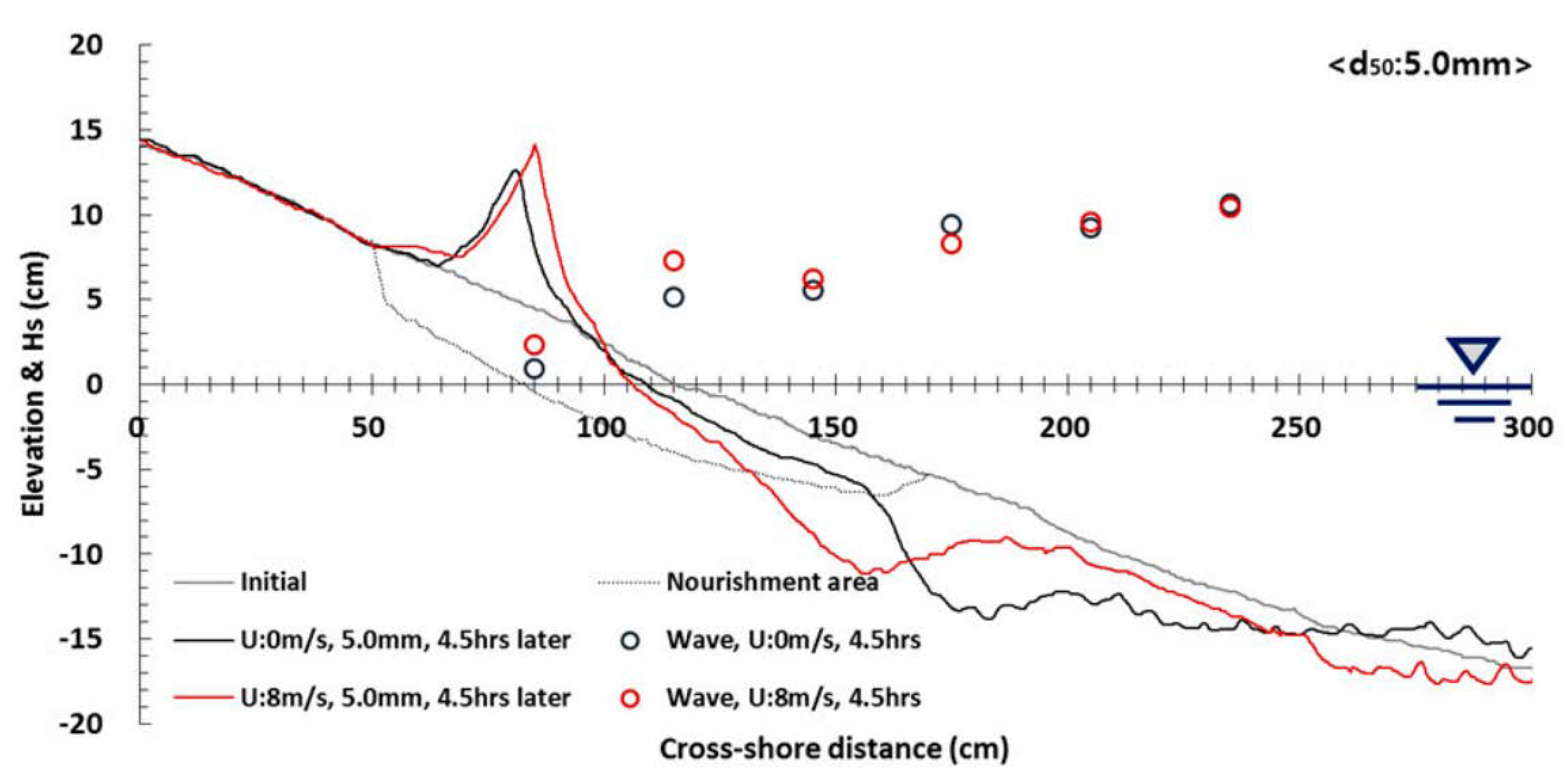
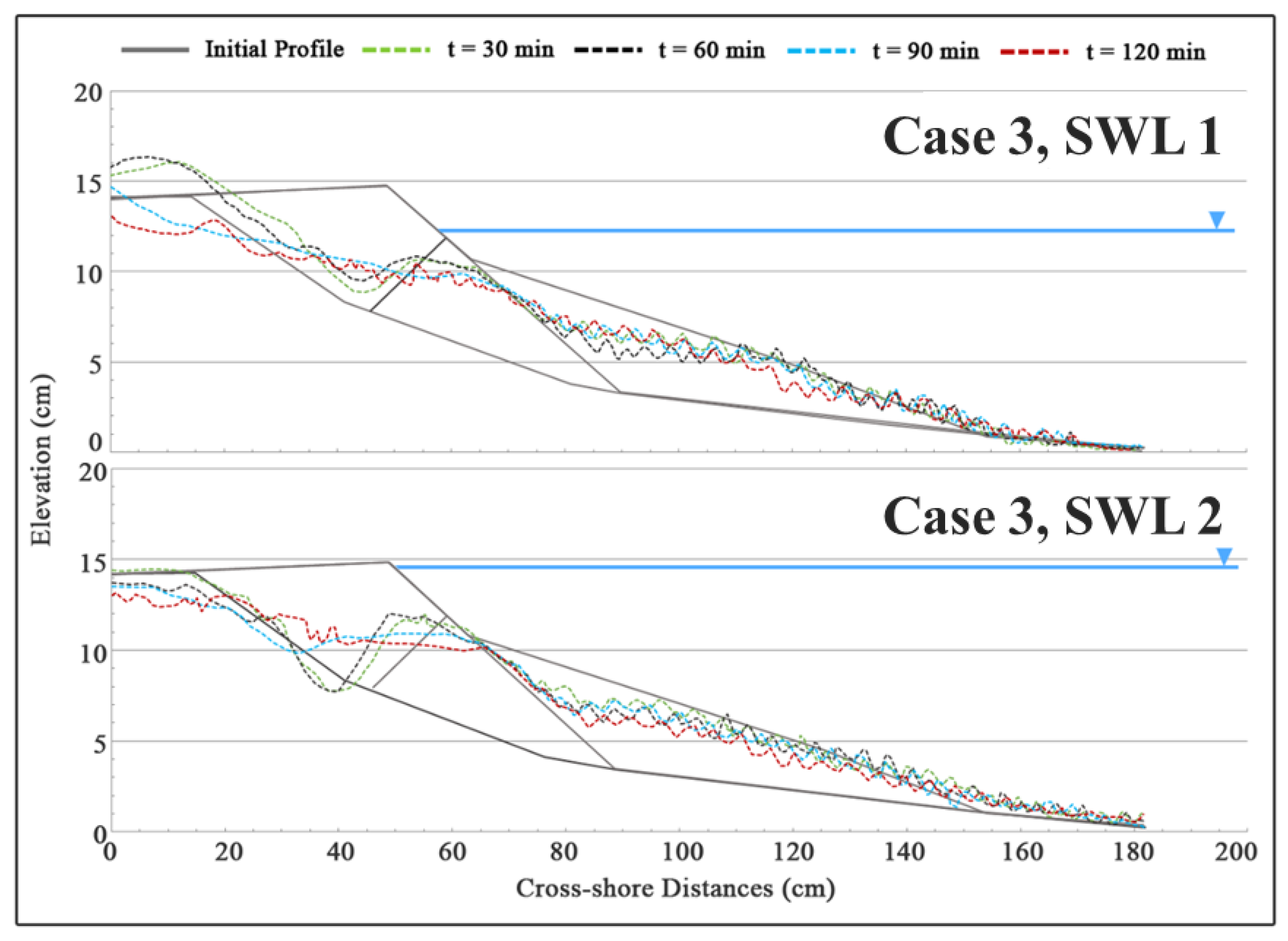
2.3. Beach Profile Evolution

The following section shows the measured profiles of test cases 1, 2, 3, and 4 at t = 0, 30, 60, 90, and 120 min for all four test cases with elevations SWL 1 and 2. For brevity, t₁ = 30 min, t₂ = 60 min, t₃ = 90 min, and t₄ = 120 min. The profiles were measured at x = 0–200 cm.

As shown in Figure 6, in test case 1 with SWL 1, a sand dune formation immediately occurred after t₁. Continuous erosion accelerated on the sand berm and, after t₃, the deposited sand dune on the backshore disappeared. Test case 1 with SWL 2 caused a trend of foreshore erosion and berm erosion during t₁ and t₂. The pattern of sand dune formation on the backshore was similar to that of test case 1 with SWL 1. However, the erosion persisted and created a deposited sand dune that disappeared faster with a higher SWL. The comparison of the two profiles showed that when using only sand as nourishment, the beaches were less sensitive to SWL, and the final profiles for SWL 1 and SWL 2 were similar.

For test case 2, with gravel berm and sand beach, Figure 7 shows the profile evolution of the measured profile at t₁ = 30 min, t₂ = 60 min, t₃ = 90 min, and t₄ = 120 min. During t₁–t₂, a gravel dune was formed on top of the berm. This gravel dune protected the minor waves from overtopping. Gravel dunes were formed on the backshore; however, because the gravel did not easily move onshore, scouring occurred on the foreshore. With time, the gravel dune migrated backshore, and the size of the dune increased. A scour trench was created landward of the berm and seaward slope, and the crest of the berm was eroded. In case 2 with SWL 2, the berm became saturated with an increase in the water level. Accordingly, the results confirmed that a large amount of erosion occurred within a short time. Compared to the results of test case 1 with SWL 1 in Figure 6, the erosion pattern showed a marked difference.

In test case 2 with SWL 1, the deposition of the berm appeared over time and the deposited gravel sand tended to retreat. This test case was found to have a good result as a countermeasure against erosion. Among the photos taken before and after Cyclone Ula at the southern part of Catalina Ramp where gravel nourishment was conducted (Figure 8), the photo on the left was taken after the gravel nourishment and before the damage caused by Cyclone Ula. The photo on the right was taken in December 2017 after Cyclone Ula, where a large amount of the gravel dune with a steep slope was formed, similar to the experimental results.

According to Shim et al. [10], gravel on the beach tends to create a gravel dune after high waves. Figure 9 shows the results reported by Shim et al. [10]. These results cannot be quantitatively compared to those of the present study because of the differences in the experimental conditions, such as incident waves, beach profile, range of beach nourishment, and generation of the wind (U). However, the experimental results for similar particle sizes can be qualitatively compared. Erosion occurred at the beginning of the experiment, but a large-scale accretion occurred on the rear side of the shoreline after a certain period. Overall, comparing the tendencies of the profile evolution, our results were similar to those of test case 2 owing to the formation of a gravel dune and foreshore erosion.

However, unlike SWL 1, SWL 2 showed berm erosion caused by sea-level rise in test case 2. The erosion problem was more pronounced in the saturated and unsaturated states than in the sand or gravel problem. The erosion pattern for the sand berm from case 1 and the gravel berm from case 2 were similar, only the pattern of deposition behind the berm was different.

With an increase in the SWL 1 to SWL 2, gravel dunes formed in different locations, with the formation of gravel dunes located on the far backshore. The scour continued and created a sand dune between the berm and the foreshore at t₂. These gravel dunes seemed to serve as protection from wave overtopping and wave overwash. Unlike in test case 1, gravel deposition and landward migration in test case 2 were sensitive to SWL, as wave run-up on gravel was sensitive to SWL. The results of this test case with SWL 2 suggest that the gravel nourishment performed at the Tuvaluan coast with a higher cyclone surge than that of Cyclone Ula.

The profile evolution in test case 3 is shown in Figure 10. As demonstrated by the initial profile with a birds eye view, gravel was hidden so that the initial profile looked the same as that in test case 1. However, the gravel layer was placed underneath the berm. Only half of the gravel used in test case 2 was applied in this test case. By the end of t₁, a tendency similar to that of test case 1 was observed. However, once the gravel layer was exposed, the gravel protected against erosion and created a gravel composite sand dune on the backshore. Over time, the beach reached equilibrium, but the gravel sand protected the beach by slowing down the erosion. After t₃, the beach profile evolution was similar to that of test case 1.

In test case 3, the gravel inside the berm formed a permeable layer. The gravel layer inside the sand berm acted as a water-permeable filter and, unlike in test case 1 which consisted of only a sand berm, it slowed the erosion rate in the area behind the gravel. This can be seen as a filter for the permeable layer of gravel and it kept the sand inside the rear section unsaturated for a period of time. Having high permeability, the gravel on the beach face caused wave water infiltration before the wave washed back to sea. Thus, the permeability helped to minimize cross-shore sediment transport and the resulting erosion. For SWL 2, erosion accelerated. However, when compared to test case 1 with SWL 2, the gravel layer was protected from the scour. In an overall comparison with SWL 1, the landward edge of the gravel layer was eroded after the berm erosion progressed landward, and the thin layer of gravel provided some protection for the sand below the gravel layer.

The profile evolution of test case 4 is shown in Figure 11. Similar to test case 3, gravel was hidden underneath the sand berm with a sill shape. The same amount of gravel was used as in test case 3. Due to the gravel sill, when the gravel was exposed, scour occurred on the sand berm. The sill’s effect became noticeable only after the sill’s crest was exposed, but wave breaking over the exposed crest created a scour hole landward of the sill. Even in the case of test case 3, the results confirmed that the gravel filter permeable layer shown in SWL 1 was not exerted at the water level of SWL 2. In the case of the buried gravel sill with SWL 2, the scour hole occurred after t₁, as wave breaking accelerated the erosion of the sand. Therefore, a dune was not formed landward and the scour hole became larger on the berm. However, the scour hole on the berm was recovered with sand after t₂.

3. Numerical Simulations and Artificial Intelligence

The recent increase in coastal storm damages necessitates the development of numerical models to predict the damage progression and breaching of beaches, coastal stone structures, and earthen levees during extreme storms. In this context, to quantitatively understand beach morphology and damage progression, robust and straightforward models are necessary to reproduce the phenomenon. However, current models cannot calculate the damage while simultaneously using different grain sizes.

Current models are based on the combinations of many physical equations and are calibrated and verified using small-scale hydraulic model experiments. Throughout the experiment, test case 1 was the only sediment of sand used, which was compared with various 2D numerical simulations. The numerical models CSHORE, SBEACH, and XBEACH were tested and compared with the results of the hydraulic model experiment and the artificial intelligence (AI) model.

In addition to test case 1, the hydraulic model experiments of test cases 2, 3, and 4, with different SWLs, were compared with the AI model’s prediction. The aim was to explore the possibility of reproducing AI convergence and its application to sediment transport. As the only data obtained from the current hydraulic model experiment were used in the AI prediction, the results may not be entirely reliable, but they can show the possibility of the application.

3.1. Artificial Neural Networks

Artificial neural networks (ANNs), a major tool in deep learning computing, are used in the areas of prediction and classification and areas where regression and other related statistical techniques have traditionally been used [11]. In general, ANNs provide either substitutive or complementary options to traditional computational schemes of statistical regression, time series analysis, pattern recognition, and numerical methods [12]. Owing to the limitations of numerical simulations reproducing gravel nourishment, ANN was used to try to predict the future profile evolution of test cases 1, 2, 3, and 4 using the hydraulic model experiment data as a training dataset. Recently, ANN was used as an alternative to nonlinear model-driven approaches. ANN relies on a data-driven approach, where the analysis depends on the available data, with little a priori rationalization of the relationships between variables and the models. The process of constructing the relationship between the input and output variables is addressed by a certain general-purpose learning algorithm.

In the present study, the ANN was inspired by information processing and communication nodes in biological systems [13]. The ANN follow the cognition process of the biological neurons of the brain and develop the intelligence from communications between different artificial neurons. It is composed of a set of interconnected artificial neurons, nodes, or a group of processing units that process and transmit information through activation functions.

The most frequently used activation functions are the linear and nonlinear functions, i.e., the logistic, rectified linear unit (ReLU), and hyperbolic tangent functions, all of which define the output of that node given an input or set of inputs.

$$f\left(x\right)=\tanh \left(x\right)=\frac{\left(e^x-e^{-x}\right)}{\left(e^x+e^{-x}\right)} \left(tanh function\right)$$

(3)

$$f\left(x\right)=\mathsf{\sigma }\left(x\right)=\frac{1}{1+e^{-x}} \left(sigmoid function\right)$$

(4)

$$f\left(x\right)=\{\begin{array}{c}0 for x \le 0 \hfill \\ x for x>0\hfill \end{array} \left(ReLU function\right)$$

(5)

The neurons of a network are structured in a single layer or multiple layers. The nodes of one layer are connected to the nodes of the next layer to which they can send information. More precisely, ANNs consist of neurons that have learnable weights and biases. Each neuron receives inputs, performs a dot product, and optionally follows it with nonlinearity. The ANN receives the input and transforms it through a series of hidden layers. As shown in Figure 12, the last connected layer is called the output layer.

Here, ANN with $O=f(\sum _{i=0}^d{w}_i{x}_i+b)$, where $x_0, x_2, x_3, \dots , x_d$ and output is $O$. Every activation function takes a single number and performs a certain fixed mathematical operation on it. Predictive analytics deals with information retrieval to predict an unknown event of interest, typically a future event. In the present study, sediment transport and profile evolution were used for the prediction. Using various data, predictive models can uncover patterns and relationships, which allow organizations to anticipate outcomes based on more concrete information than an assumption. The advantage of ANNs is the feedforward networking and backpropagation of error [14], by which the network can be trained to minimize the error up to an acceptable accuracy. The training procedure of the network is selected to fit the purpose of the supervised and unsupervised training types. In this study, a backpropagation algorithm with supervised learning was used.

3.2. Dataset and Architecture of the ANN Model

Each hidden layer consists of a set of neurons. Each neuron is fully connected to all neurons in the previous layer, and the neurons in a single layer function entirely independently and do not share any connections. The last fully connected layer is called the output layer. The architecture of this research is based on a three-layer perceptron (see Figure 13). Seven nodes with an input layer and three hidden layers with 254 nodes were used. The intention was to obtain the final predicted profile, so the node of the output layer was set to one. The aim was to predict the future profile and compare it with the measured data obtained from hydraulic model experiments. Thus, the beach profile evolution with t₁, t₂, and t₃ was used for the training, and t₄ was tested with the output from the prediction.

As in the architecture of the ANN model shown in

Table 2. Architecture of the present study.

Parameter	LAF Case	RAF Case	SAF Case
Model	Deep Neural Network
Input parameter	Cross-shore distance (value)
	Initial profile
	Time
	Height
	Period
	Case
	Sea Water Level
Activation function	Linear	ReLU		sigmoid
Hidden layer	3
Hidden layer’s node	254
Output node	1
Target	Change Profile

, seven input parameters were used for training and testing. The profiles of test cases 1, 2, 3, and 4 with SWL 1 and 2 for times t₁, t₂, and t₃ were trained. Seven input parameters, i.e., cross-shore distance, initial profile, time, height, period, case, and seawater levels, with the output (profile evolution) were used in the training. For the testing (t₄ of each test case), the same input parameters were used to obtain the final profile evolution as an output. Afterward, the tested outputs were compared with the measured profiles and the differences were analyzed to determine the performance of the ANN model, as shown in

Table 3. Results of the RMSE, MAE, and MSE (ReLU activation function).

SWL	CASE	RMSE	MAE	MSE
SWL 1	1	0.6141	0.6141	0.7235
	2	1.3004	1.3004	3.9409
	3	0.9777	0.9777	1.9097
	4	0.8903	0.8903	1.9033
SWL 2	1	0.7559	0.7559	0.9443
	2	0.8308	0.8308	1.2265
	3	0.5345	0.5345	0.4829
	4	0.6398	0.6398	0.7698

.

The performance of the developed ANN model was evaluated to ensure that the model could perform within the predefined limits set by the data used for training. The conventional approach was used to evaluate the model performance on an independent validation set of data not used in the training process. The root mean square error (RMSE), mean absolute error (MAE), and mean squared error (MSE) were used as evaluation metrics to gauge the prediction accuracy, which are defined as follows (Equations (6)–(8)):

$$RMSE=\sqrt{\frac{{\sum }_i^n{\left(Predicte{d}_i-Actua{l}_i\right)}^2}{n}}$$

(6)

$$MAE=\frac{1}{n}{\sum }_i^n\left|Predicte{d}_i-Actua{l}_i\right|$$

(7)

$$MSE=\frac{1}{n}{\sum }_i^n{\left(Predicte{d}_i-Actua{l}_i\right)}^2$$

(8)

where n is the number of test samples, Predicted is the predicted beach profile change at t₄ = 120 min, and Actual denotes the measured t₄ from the hydraulic model experiment.

From the prediction accuracy comparison of using the activation function of LAF, RAF, and SAF cases, none of the three activation functions had significant differences in error because the amount of the training data was not too large. However, the ReLU activation function was chosen because ReLU is a faster learning activation function, which was proven to be the most successful and widely used function [15], and its data sparsity reduces the likelihood of gradient vanishment.

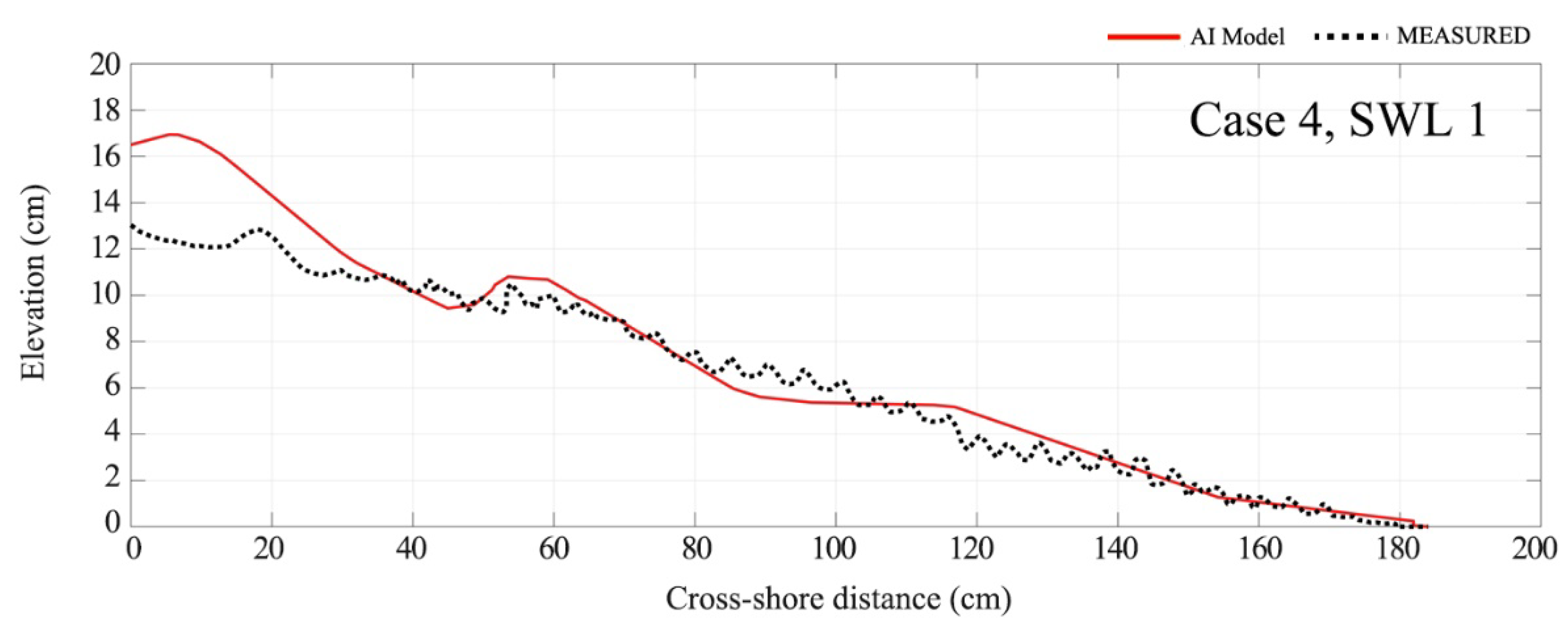
3.3. AI (ANN) Model Results

The ANN model was used to predict the future profile evolution of the sediment transport of the sand and gravel nourishment of the test cases (cases 1–4). The final beach profile for t₄ = 120 min was compared to that of the hydraulic model experiment. Some drawbacks associated with the practical use of the ANN include the possibly long modeling process time and the large amount of data required.

As shown in Figure 14 and Figure 15, in test case 1, using only sand nourishment, SWL 1 and SWL 2 were compared. This profile is the equilibrium beach profile, where the ANN model effectively predicted the foreshore. Due to the lack of data to be trained except for the three time steps t₁, t₂, and t₃, some differences were observed. Nonetheless, the overall profile appeared to be reasonable.

The typical gravel nourishment of Tuvalu was reproduced and tested using test case 2. Figure 16 and Figure 17 show the results of the ANN model and compare the profiles. From SWL 1, the ANN model produced a dune on top of the berm, similar to the measured profile. However, the shape and location were not in the exact same location. For the sake of tendency, creating the dune on top of the berm and foreshore erosion were accurately reproduced through the ANN. The measured profile of test case 2 with SWL 2 showed dune formation on the backshore, and the ANN model also predicted the berm shape profile on the backshore.

In test case 3 with SWL 1, shown in Figure 18, the ANN model predicted less erosion on the backshore compared to the measured profile evolution. Although the overall tendency of the beach profile to reach equilibrium was predicted, the amount of erosion was not accurately predicted. Nonetheless, the prediction of the ANN for test case 3 with SWL 2 in Figure 19 was more accurate than the case 3 with SWL 1 prediction. Erosion was accurately predicted for the berm and foreshore.

Finally, Figure 20 and Figure 21 show the prediction results of Case 4 with SWL 1 and 2. For test case 4 with SWL 1, the scour hole was predicted on the berm and less erosion was predicted on the backshore of the beach. As shown in Figure 20, the foreshore prediction of the 60–180 cm cross-shore was accurate. The gravel sill did not move as much on the 40–64 cm cross-shore in the measured data, but the tendency of the ANN prediction in this section was predicted well. The prediction presented a dune shape formed in this section, unlike the measured data. The 0–40 cm cross-shore had a reasonable prediction compared to the measured data.

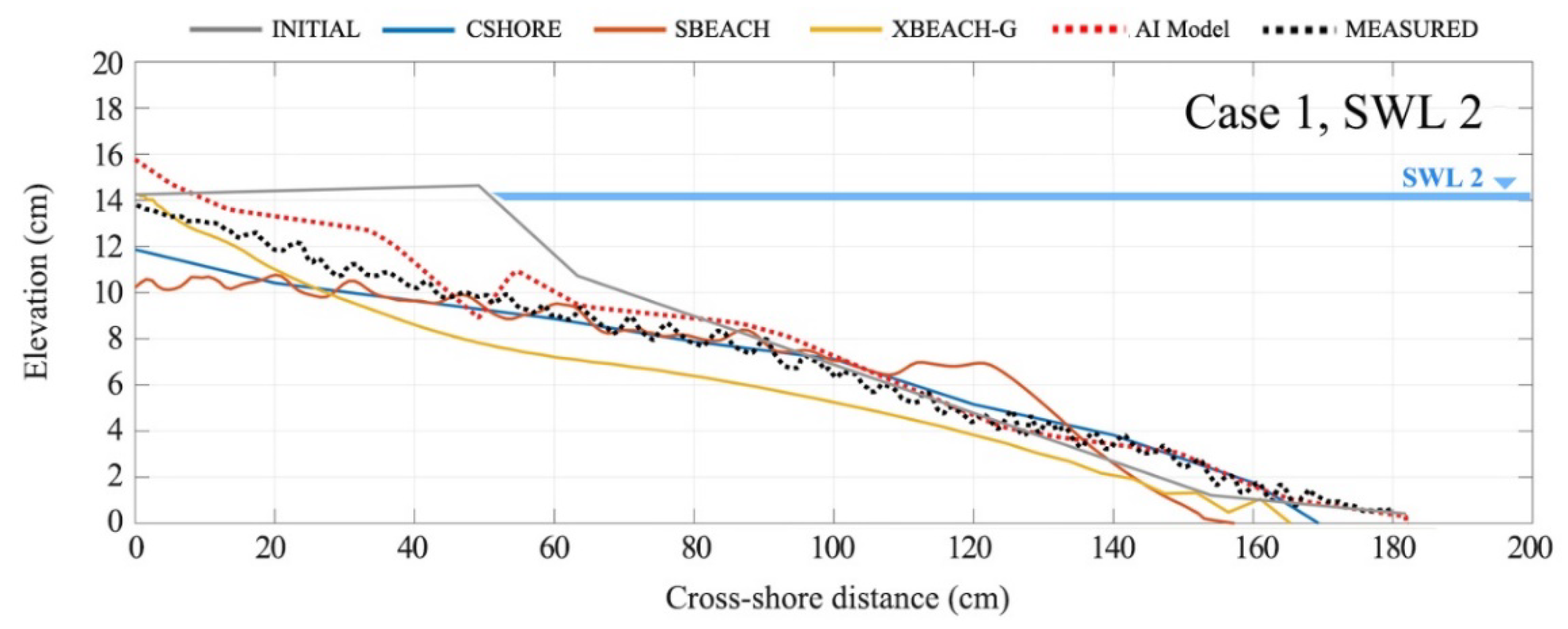
3.4. Numerical Simulations and Comparisons

Numerous numerical models for the littoral zone have been proposed for sediment transport profile behavior [16]. For instance, in a pioneering study on beaches along the Danish North Sea coast and the California coast, Bruun [17] developed a predictive equation for the equilibrium beach profile. Furthermore, using the wave energy approach and differentiation between the bedload and suspended load, Bagnold [18] developed formulas to calculate sediment transport rates, including cross-shore transport. Several subsequent studies, including Bailard [19] and Stive and De Vriend [20], refined Bagnold’s work [18]. Using a combination of theory and field observations, Larson [21] proposed the SEBACH model to predict profile changes due to storms, and the CSHORE model was used to predict such changes in response to the interactions between waves and currents. Finally, the XBEACH mode, which uses nonlinear shallow water equations, was proposed.

The aim of this section is not to compare and determine which model is the best but to examine whether the AI model can reproduce a reasonable prediction similar to other numerical simulations. All the three numerical models used 0.16 mm for D₅₀ and irregular waves with the same wave heights and wave period used in the hydraulic model experiment. All models used the smallest number of calculation cells or grid sizes as possible.

For SWL 1 in Figure 22, all models accurately predicted the profile evolution for the measured profile at t₄ = 120 min. When comparing these results with those of the ANN model prediction, the ANN model prediction was more accurate with the same tendency of becoming an equilibrium profile. When the SWL increased to SWL 2 (Figure 23), the prediction of the numerical simulations was less accurate. The erosion was overestimated for CSHORE. SBEACH predicted too much deposition on the foreshore, whereas XBEACH-G predicted too much erosion compared to the other models. This may be a problem when the SWL is too high. The ANN prediction was not perfect, but it was sufficiently good. The use of large amounts of small and field-scale data will increase the accuracy of the current ANN model, highlighting the potential of AI applications on the sediment transport prediction of beaches where numerical simulation cannot predict.

4. Conclusions

A laboratory experiment consisting of four test series was conducted in a wave flume with a sand beach and a nourished berm to compare the effectiveness of each test case. The SWL was increased to generate extreme conditions to create accretional profile changes on the foreshore and berm. While test case 1 was vulnerable to extreme wave conditions and quickly became an equilibrium profile, test case 2, with its gravel berm, showed deposition of the berm over time and had a good result as a countermeasure against erosion. For aesthetic and environmental purposes, test cases 3 and 4 were tested. Gravel underneath the berm acts as a filter for the permeable layer of gravel and keeps the sand inside the rear section unsaturated for a period of time. Although the water-permeable layer is generally effective when there is no sealevel rise, the gravel water-permeable layer has a similar effect even when the sea-level rise is confirmed through this research.

ANNs were used to predict the final profiles. Throughout the profile comparisons of ANNs and measured data for the final profile, the ANN model predicted the tendency of the erosion quite well, forming the dune on the backshore even when using gravel nourishment.

When gravel and sand are mixed, such as gravel nourishment, it is challenging to draw results other than the hydraulic model experiment. Throughout the research, the application of AI in coastal engineering started with the question, “if one can create a robust AI model using various hydraulic model experiments and field data as big data, can it be possible to replace the limitations of the numerical simulations composed of mathematical formulas?”. The results of this study may be minimal, but the results were good enough and thought to be an excellent initial step to deepen the convergence of AI in coastal engineering.

The prediction of the ANN model for the erosion trend was accurate, but the amount was smaller. This limitation could have been caused by the size of the dataset used for model training. In future analyses, more datasets with shorter timesteps and small- and large-scale experiments should be trained on the model to increase the prediction accuracy. Moreover, various tests with various types of beach profiles should be trained to make the ANN model more robust and accurate for practical use.

References

1. Lopez, I.; Aragones, I.; Villacampa, Y.; Gonzalez, F.J. Gravel beach nourishment: Modelling the equilibrium beach profile. Sci. Total Environ. 2017, 619–620, 772–783. [Google Scholar] [CrossRef] [PubMed] [Green Version]
2. National Research Council. Beach Nourishment and Protection; National Academy Press: Washington, DC, USA, 1995. [Google Scholar]
3. Wieser, W. The effect of grain zize on the distribution of small invertebrates inhabiting the beaches of Puget Sound. Limnol. Oceanogr. 1953, 4, 181–194. [Google Scholar] [CrossRef] [Green Version]
4. Kumada, T.; Uda, T.; Matsuura, T.; Sumiya, M. Field Experiment on Beach Nourishment Using Gravel at Jinkoji Coast. In Proceedings of the 32nd Conference on Coastal Engineering, Shanghai, China, 30 June–5 July 2010; pp. 1–13. [Google Scholar]
5. Cammelli, C.; Jackson, N.L.; Nordstrom, K.F.; Pranzini, E. Assessment of a gravel nourishment project fronting a seawall at Marina di Pisa, Italy. J. Coast. Res. 2006, 2, 770–775. [Google Scholar]
6. Cohen, O.; Anthony, E.J. Gravel beach erosion and nourishment in Nice, French Riviera. Mediterranee 2007, 108, 99–103. [Google Scholar] [CrossRef]
7. Onaka, S.; Ichikawa, S.; Izumi, M.; Uda, T.; Hirano, J. Effectiveness of gravel beach nourishment on Pacific Island, world scientific. Asian Pac. Coasts 2017, 2017, 651–662. [Google Scholar]
8. Kim, H.D.; Kim, K.H.; Aoki, S.; Koo, S.; Kwak, K. Gravel beach nourishment at a low-wave energy environment to control the effects of global warming. Coast. Sediment. 2019, 19, 329–337. [Google Scholar]
9. Noble, D.R.; Draycott, S.; Thomas, A.; Bruce, T. Design diagram for wavelength discrepancy in tank testing with inconsistently scaled intermediate water depth. Int. J. Mar. Energy 2017, 18, 109–113. [Google Scholar] [CrossRef]
10. Shim, K.T.; Kim, K.H.; Park, J.H. The effectiveness of adaptive beach protection methods under wind application. J. Mar. Sci. Eng. 2019, 7, 387. [Google Scholar] [CrossRef] [Green Version]
11. Abambres, M.; Ferreira, A. Application of ANN in pavement engineering: State-of-Art. HAL 2017, hal-0200668v2. [Google Scholar] [CrossRef]
12. Konate, A. Artificial neural network: A tool for approximating complex functions. HAL 2019, hal-020759. [Google Scholar]
13. Salahudeen, A.B.; Ijimdiya, T.S.; Eberemu, A.O.; Osinubi, K.J. Artificial neural networks prediction of compaction characteristics of black cotton soil stabilized with cement kiln dust. J. Soft Comput. Civil. Eng. 2018, 2, 50–71. [Google Scholar]
14. Matuszewski, J.; Sikorska-Lukasiewicz, K. Neural network application for emitter identification. In Proceedings of the 18th International Radar Symposium (IRS), Prague, Czech Republic, 28–30 June 2017; pp. 1–8. [Google Scholar]
15. Ramachandran, P.; Zoph, B.; Le, Q. Searching for activation functions. arXiv 2017, arXiv:1710.05941. [Google Scholar]
16. Yuan, F. Cross-Shore Beach Morphological Model for Beach Erosion and Recovery. Ph.D. Thesis, School of Civil and Environmental Engineering, UNSW University, Sydney, NSW, Australia, 2017. [Google Scholar]
17. Bruun, P. Coastal erosion and the development of beach profiles. In Beach Erosion Board Technical Memo No. 44; US Army Engineer Waterways Experiment Station: Vicksburg, MS, USA, 1954. [Google Scholar]
18. Bagnold, R.A. An Approach to The Sediment Transport Problem from General Physics; Geological Survey Professional Paper 422-1; United States Government Printing Office: Washington, DC, USA, 1996. [Google Scholar]
19. Bailard, J.A. Modeling On-Offshore Sediment Transport in the Surfzone. In Proceedings of the 18th International Conference on Coastal Engineering, Cape Town, South Africa, 14–19 November 1982. [Google Scholar]
20. Stive, M.J.F.; De Vriend, H.J. Quasi-3D nearshore current modelling: Wave-induced secondary current. In Proceedings of the Coastal Hydrodynamics, ASCE, Newark, DL, USA, 28 June–1 July 1987; pp. 356–370. [Google Scholar]
21. Larson, M. A model of beach profile change under random waves. J. Waterw. Port. Coast. Ocean. Eng. 1996, 122, 172–181. [Google Scholar] [CrossRef]
Figure 1. Wave flume used in the hydraulic model experiment.
Jmse 09 00600 g001
Figure 2. Gravel nourishment typical cross section on the Fongafale shore.
Jmse 09 00600 g002
Figure 3. Wave height at the lagoon side during the monitoring period.
Jmse 09 00600 g003
Figure 4. Four test cases with two SWLs tested with 120 min runs each.
Jmse 09 00600 g004
Figure 5. Initial profiles of test cases 1, 2, 3, and 4.
Jmse 09 00600 g005
Figure 6. Case 1 with SWL 1 and SWL 2 profile evolution at t1, t2, t3, and t4.
Jmse 09 00600 g006
Figure 7. Case 2 with SWL 1 and SWL 2 profile evolution of t1, t2, t3, and t4.
Jmse 09 00600 g007
Figure 8. Southern part of Catalina Ramp with gravel nourishment.
Jmse 09 00600 g008
Figure 9. Experiment of the gravel nourished beach [10].
Jmse 09 00600 g009
Figure 10. Case 3 with SWL 1 and SWL 2 profile evolution of t1, t2, t3, and t4.
Jmse 09 00600 g010
Figure 11. Case 3: BGL with SWL 1 and SWL 2 profile evolution of t1, t2, t3, and t4.
Jmse 09 00600 g011
Figure 12. Structure of neurons of the network.
Jmse 09 00600 g012
Figure 13. Neural network architecture used in the present study.
Jmse 09 00600 g013
Figure 14. Case 1 SWL 1 comparison of the ANN prediction and measured from the physical test.
Jmse 09 00600 g014
Figure 15. Case 1 SWL 2 comparison of the ANN prediction and measured from the physical test.
Jmse 09 00600 g015
Figure 16. Case 2 SWL 1 comparison of the ANN prediction and measured from the physical test.
Jmse 09 00600 g016
Figure 17. Case 2 SWL 2 comparison of the ANN prediction and measured from the physical test.
Jmse 09 00600 g017
Figure 18. Case 3 SWL 1 comparison of the ANN prediction and measured from the physical test.
Jmse 09 00600 g018
Figure 19. Case 3 SWL 2 comparison of the ANN prediction and measured from the physical test.
Jmse 09 00600 g019
Figure 20. Case 4 SWL 1 comparison of the ANN prediction and measured from the physical test.
Jmse 09 00600 g020
Figure 21. Case 4 SWL 2 comparison of the ANN prediction and measured from the physical test.
Jmse 09 00600 g021
Figure 22. Case 1 SWL 1 comparison of the numerical simulations and the ANN model.
Jmse 09 00600 g022
Figure 23. Case 1 SWL 2 comparison of the numerical simulations and the ANN model.
Jmse 09 00600 g023