


Abstract
Wind and waves present the main causes of environmental loading on seagoing ships and offshore structures. Thus, its detailed understanding can improve the design and maintenance of these structures. Wind and wave statistical models are developed based on the WorldWaves database for the Adriatic Sea: for the entire Adriatic Sea as a whole, divided into three regions and for 39 uniformly spaced locations across the offshore Adriatic. Model parameters are fitted and presented for each case, following the conditional modelling approach, i.e., the marginal distribution of significant wave height and conditional distribution of peak period and wind speed. Extreme significant wave heights were evaluated for 20-, 50- and 100-year return periods. The presented data provide a consistent and comprehensive description of metocean (wind and wave) climate in the Adriatic Sea that can serve as input for almost all kind of analyses of ships and offshore structures.
1. Introduction
Wave (re-analysis) databases, comprising numerical wave model hindcasts and assimilated altimetry satellite data, present a comprehensive state-of-the-art source for analysis of metocean data that serve as input for the design and assessment of oceangoing vessels and offshore structures [1]. The WorldWaves database was used in this study to derive wind and wave statistics for the Adriatic Sea, which is a semi-enclosed sea basin with specific wind–wave climate. The basin is analyzed as a whole, divided into three regions and at 39 evenly spaced locations. Procedures and concepts applied in the study resulted with environmental wind and wave models that provide a detailed and structured insight into the wind–wave climate of this basin. Joint probability distributions of significant wave height and peak periods and distribution of wind speed to significant wave height are developed together with extreme wave height estimation for 20, 50 and 100 year return periods.
The obtained results are useful for the design, operation planning, maintenance and life-time extension of marine-related engineering objects in the Adriatic. Specific calculations such as: extreme sea states analysis for the design of marine structures [2], coupled aero- and hydro-dynamic analysis of floating offshore wind turbines [3], long-term fatigue calculations [4], structural reliability [5] and mooring analyses [6], can benefit from the input of the developed data. Wave statistics in the Adriatic is also used for exploring wave energy potential [7,8] and for planning and evaluating the performance of high-requirement service vessels such as the coastal patrol boat developed for the Adriatic [9]. Safety analysis of a fishing vessel due to roll in a seaway [10] and organization of special marine operations [11] are other examples where accurate wave statistics for the Adriatic is indispensable.
In the second half of 20th century, wave statistics in the Adriatic was based on visual observations collected from merchant and meteorological vessels and published in the wave climatology atlas [12]. Wave statistics was rather roughly graphically presented in the form of wave roses that were later digitalized and studied in terms of extreme values [13]. These data, however, suffer from known inaccuracies of visual wave observations and lack of extreme events due to heavy weather avoidance by ships [14]. Later, measurements have been performed from four floating buoys installed along the west coast of the Adriatic [15]. However, these data were recorded and are available only for limited time of 5 years, with some interruptions due to failure and maintenance. One of the most comprehensive wave-data sources in general are the measurements from the Aqua Alta oceanographic tower, located near Venice in the north part of the Adriatic [16]. Although 38 years of continues uninterrupted measurements are available, they refer only to one specific location and cannot be used for the whole Adriatic Sea.
The present study represents the first complete wave and wind statistics for the whole Adriatic Sea, representing progress compared to previous studies [17]. The way the data are presented enables its application to almost all purposes related to marine structural design and analysis, as reviewed in the preceding paragraphs. Site specific design (e.g., for offshore structures) might require spatial interpolation of presented data; however, it can be directly applicable for the analysis of ships, as they are not confined to a specific location. Particular attention is paid to the accuracy of calculated extreme values, to avoid too conservative results that could lead to non-economical and over-dimensioned structures [18].
The paper is organized as follows. Initially, the WorldWaves database, used as the underlying material for the study, is described in Section 2 along with preliminary data structuring such as the development of sea-state and wind contingency tables, wave roses visualizations and example validations against existing buoy data. In Section 3 the theoretical background of applied methods is presented for the development of the joint probability distribution models. In Section 4, all model parameters and extreme values are presented graphically, both regionally and per individual location analyzed. Section 5 gives a discussion on the results and Section 6 presents the conclusion. At the end of the paper, Appendix A provides basic data, such as location coordinates and regional subdivision and Appendix B gives detailed tabulated results that are graphically presented in Section 4.
2. Data
The underlying data used for the analysis of wave and wind climate analysis in the Adriatic Sea were extracted from the WorldWaves (WW) database. The database represents numerical wave model hindcasts with assimilated available satellite altimetry measurements [19,20]. It includes 39 locations, evenly distributed across the Adriatic Sea with 0.5° × 0.5° (lat.-long.) spacing, in the period from September 1992 to January 2016. The underlying numerical wave model WAM (Wave Modelling) is run at the ECMWF (European Centre for Medium-Range Weather Forecasts) which acts as a European meteorological institute providing numerical atmospheric and ocean forecasts, archiving data and improving forecasting models. WAM is extensively validated in the literature [21,22]. Satellite altimetry measurements are, in general, validated by in-situ measurements made with wave buoys and are considered an empirical source of data for larger domains but lack in continuity as they are confined by individual satellite tracks and overflight times. WW includes satellite altimetry data from satellite missions taking measurements over the Mediterranean (i.e., the Adriatic): European Remote Sensing Satellites (ERS-1 and ERS-2), Ocean Topography Experiment (TOPEX), Geosat Follow-On, Jason and Environmental Satellite (Envisat).
WW Data Subdivision, Preparation and Preliminary Considerations
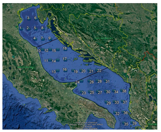
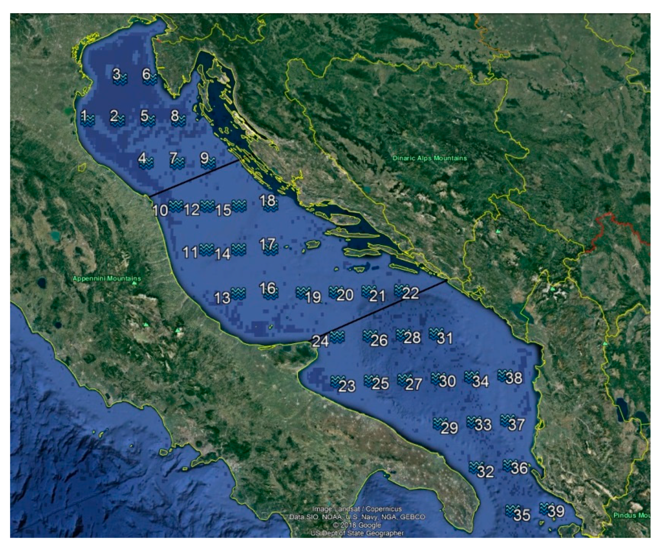
A total of 39 locations were available within the WW database for the Adriatic Sea. The locations were analyzed: individually, grouped into regions (southern, central and northern Adriatic, according to DHMZ–Croatian Meteorological and Hydrological Service official subdivision) and joint together for the basin as a whole. Location, their numbering and regional subdivision are presented in Figure 1, and exact geographic coordinates are given in Appendix A Table A1.
Figure 1.
Studied locations in the Adriatic Sea as available from the WW database.
At each location, 12 physical wave and wind parameters are available at 6-h intervals (four per day) as presented in Appendix A Table A2 and for each location there are total of 34,460 lines of records.
Maximum recorded significant wave heights, along with accompanying parameters, were extracted and are presented in Appendix A Table A3. The single highest significant wave height in the database is recorded at location 9 (E14.5°–N44.0°) 16.11.2002, reading Hs = 6.72 m during southeast wind (local names jugo/scirocco). For comparison, the single highest wave measured until now along the east coast reads Hmax = 10.87 m off the city of Dubrovnik on 12.11.2019, associated with the significant wave height of Hs = 4.75 m. The highest significant wave height so far is measured from the gas platform in the north Adriatic and reads 7.5 m [23].
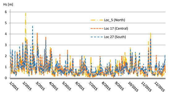
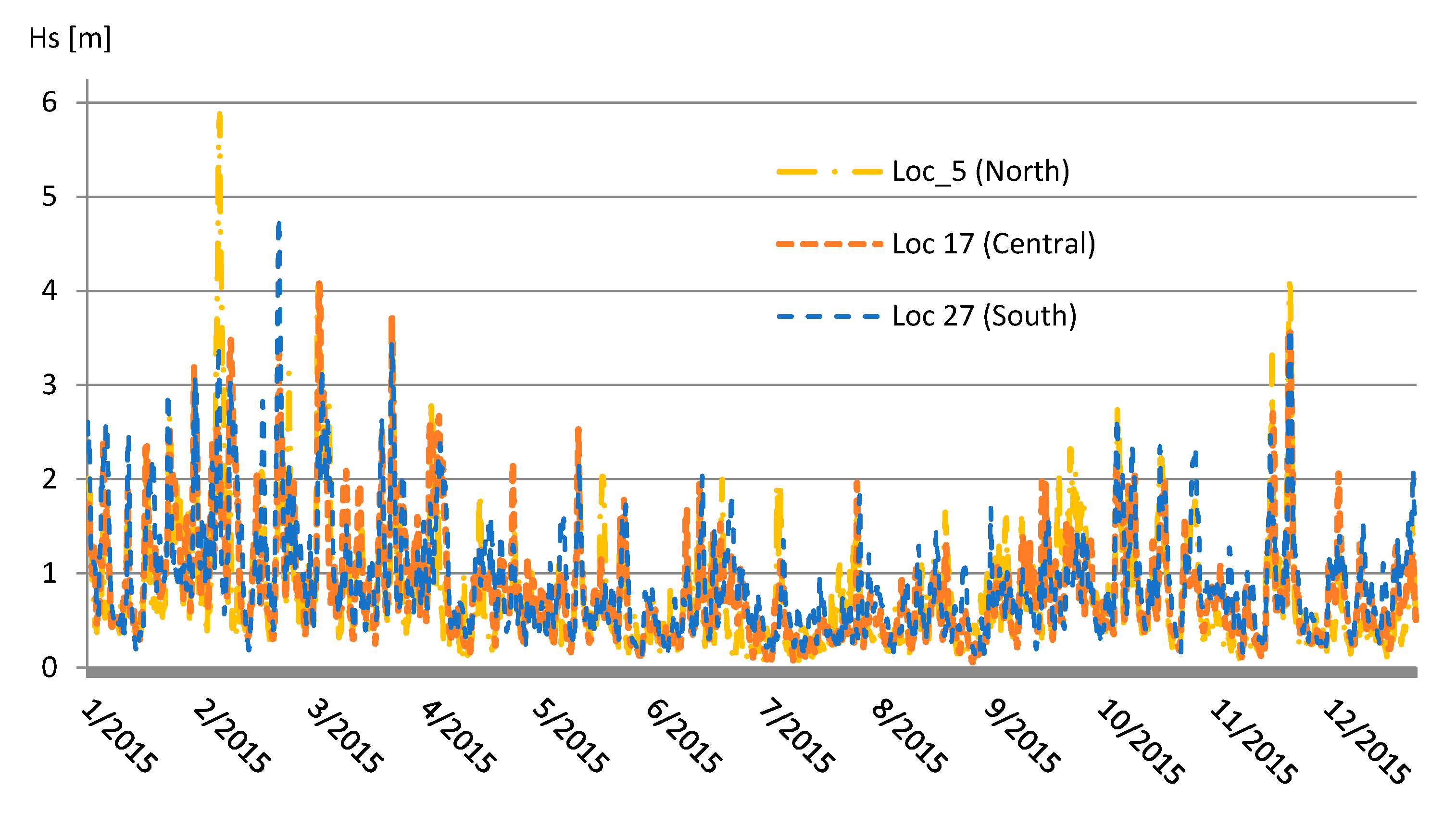
Visualization of Hs time series for a one-year period, presented in Figure 2, confirms expected higher variability during winter months.
Figure 2.
Hs time series during 2015 at three locations, in North, Central and South Adriatic.
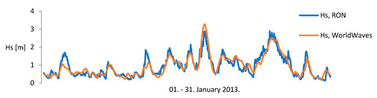
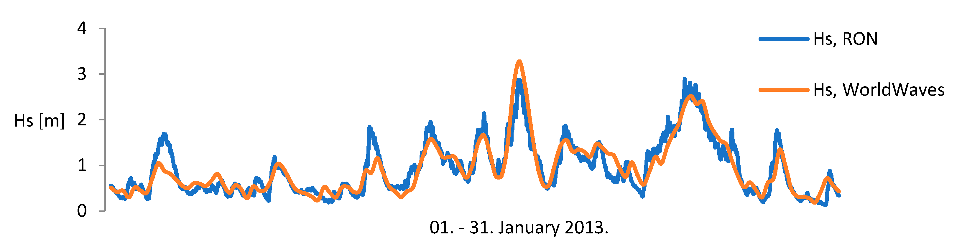
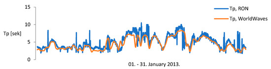
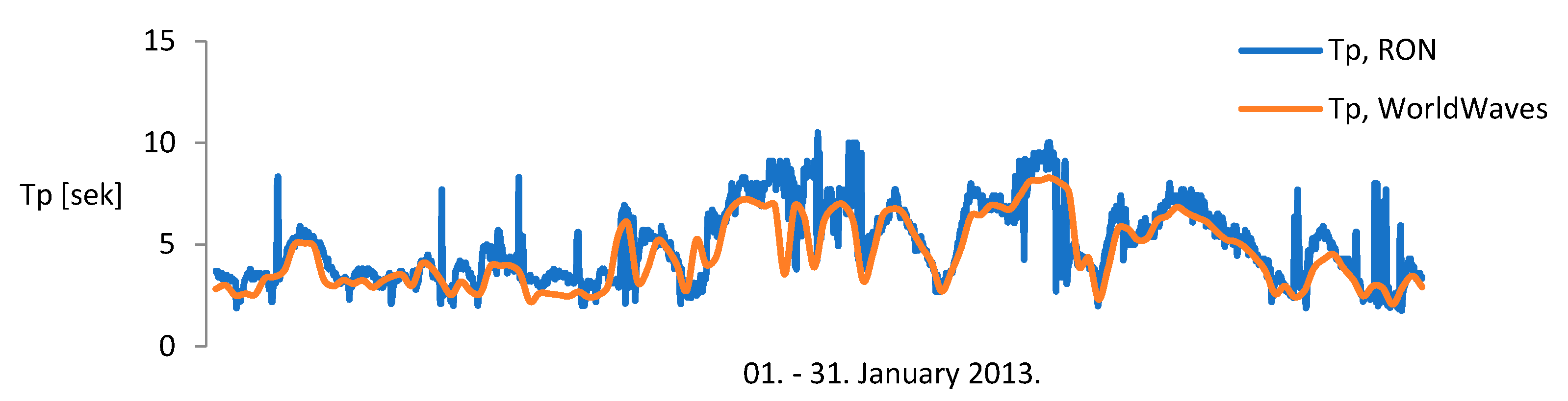
An example validation of WW data against available in-situ wave buoy measurement data from the Italian RON project [15] is shown for Hs and Tp on locations nearby for one winter month period, in Figure 3 and Figure 4.
Figure 3.
Hs time series from WW database (location 4) and RON buoy “Ancona” (13°43′10″ E–43°49′26″ N).
Figure 4.
Tp time series from WW database (location 4) and RON buoy “Ancona” (13°43′10″ E–43°49′26″ N).
The WW and RON locations compared in Figure 3 and Figure 4 are about 26 km apart. The time series shows a good match, especially for significant wave heights. General Hs trends match well and peaks coincide. Variations between extremes in Figure 3 can be accounted to distance between the compared locations (with influence of the coastline and surrounding orography), to physical and numerical limitations and settings of the numerical model and measurement buoy properties. Deviations between wave period Tp records are slightly larger than for Hs. Buoy data for wave periods show local “jumps” which could suggest that the buoy data possibly need additional filtering.
To prepare the data for analysis, the following frequency of occurrence tables were extracted from the WW database:
- Sea state tables (Hs–Tp), for the following:
- The Adriatic Sea with all location merged as presented in Table 1;
- Adriatic regions as presented in Appendix A (North, Table A4; Central, Table A5; and South, Table A6);
- Each of the 39 locations individually.
Table 1. Sea state table–entire Adriatic Sea basin, period September 1992–January 2016. - Wind speed to significant wave height (uw–Hs), for the following:
- The Adriatic Sea with all location merged as presented in Table 2;
- Adriatic regions (North, Central and South) as presented in Appendix A (North, Table A7; Central, Table A8; and South, Table A9);
- Each of the 39 locations individually.
Table 2. Wind speed—significant wave height occurrence—entire Adriatic, Sept 1992–Jan 2016.
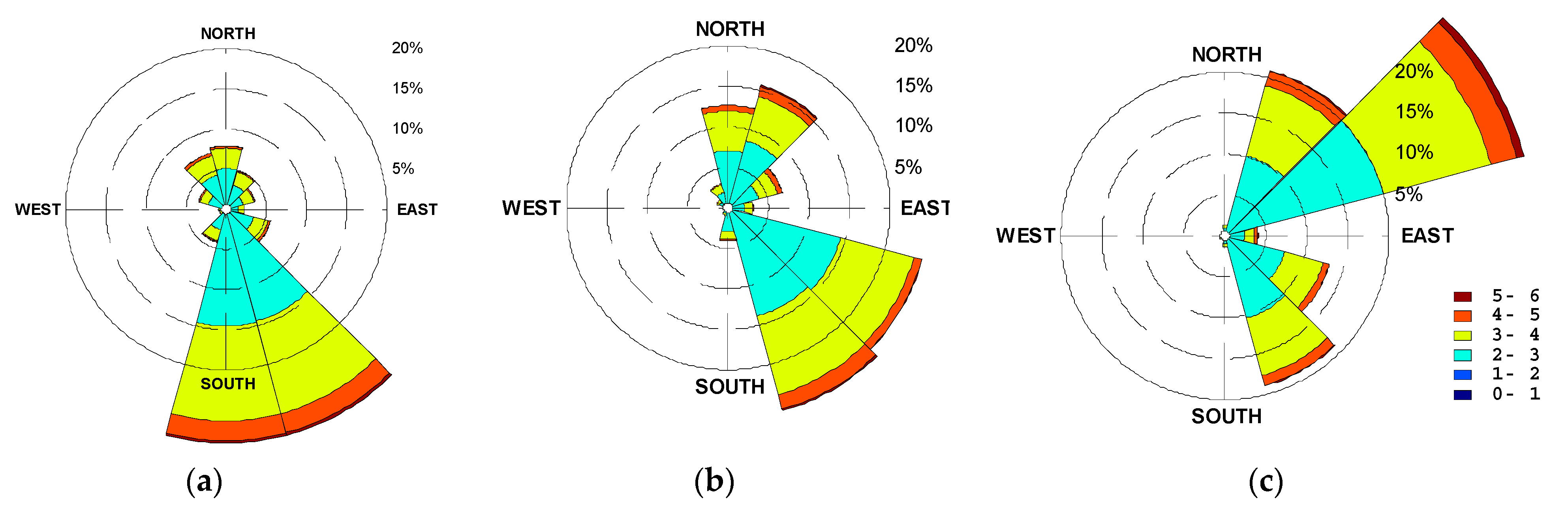
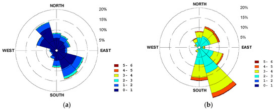
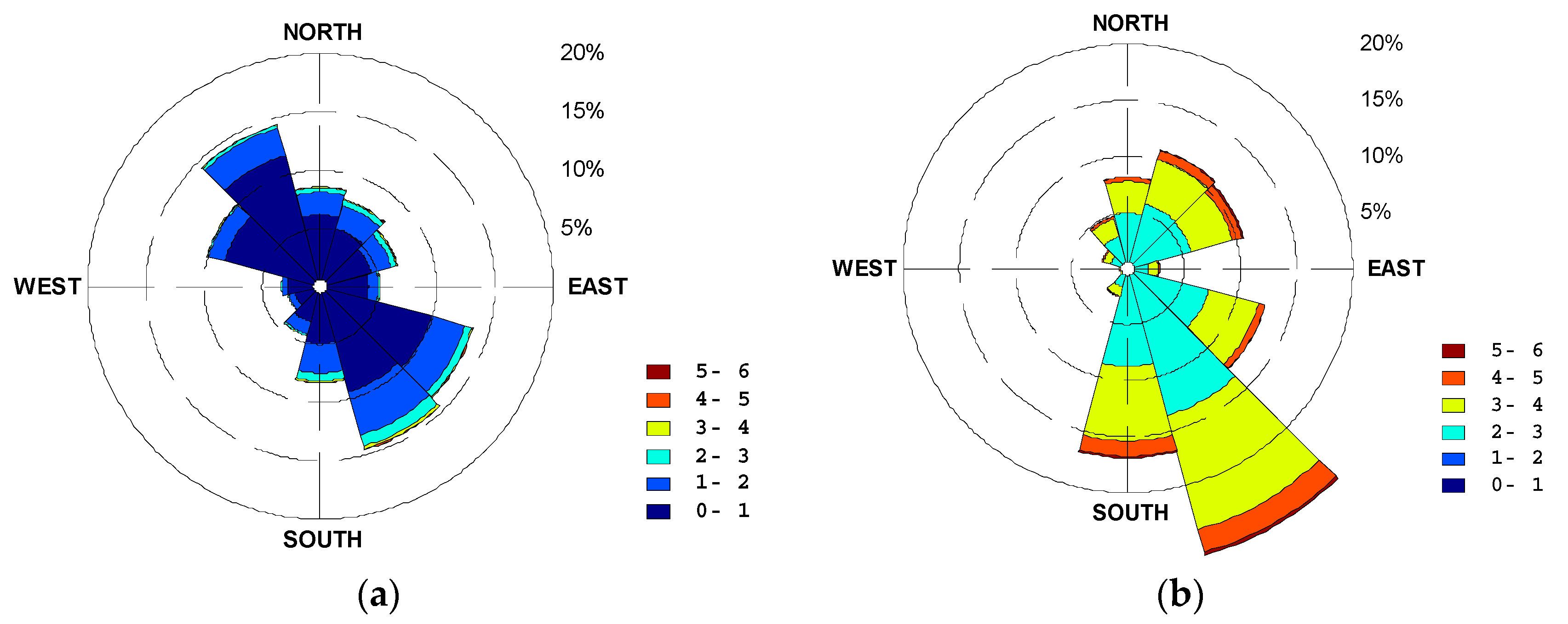
Additionally, the well-known directionality of higher wave height associated with S-SE winds (jugo/scirocco) and NE winds (bura/bora), as the Adriatic basin specificities due to the surrounding orography, is confirmed by wave roses. Wave roses for the Adriatic as a whole are presented in Figure 5.
Figure 5.
Wave roses for the entire Adriatic basin: (a) all sea states and (b) sea states with Hs > 2.5 m.
There is a noticeable amount of smaller N–NW waves accounted to the same direction (maestral/maestrale) wind—a typical daily coastal circulation, caused by temperature oscillation between land and sea during summer months, which is important to the leisure nautical sector due to its predictability and mild character. Regional wave roses are available in Appendix A Figure A1 and Figure A2 and suggest higher dominance of S–SE waves in South and Central Adriatic and NE high wave dominance in the North Adriatic region.
3. Methods
The WW data were analyzed in accordance with Det Norske Veritas (DNV) classification society recommendations for determining environmental conditions and loads on marine structures [2]. A joint distribution is applied, consisting of a marginal three-parameter Weibull distribution of significant wave heights and a conditional log-normal distribution for peak periods. For wind speeds, a conditional distribution is given as function of significant wave height and described by a two-parameter Weibull distribution.
3.1. Joint Distribution of Significant Wave Height and Peak Periods
Based on sea state tables, both regional and per individual location, a joint probability distribution model was derived with the aim to optimize the parameters that will later be used to determine extreme sea states for return periods longer than the database span and to provide a consistent approach for determination of loads for fatigue and strength analyses of ships and offshore structures.
CMA approach (Conditional Modelling Approach) is applied for modelling the joint distribution of significant wave height and peak (spectral) period. In general, this method defines the probability density function (PDF) by a marginal distribution and a set of conditional probability densities, each of which is modelled by a parametric function whose parameters are optimized by mathematical fitting techniques to represent data from the WW database in the best possible way. The CMA approach of fitting joint distribution to the wave data was first proposed by Bitner-Gregersen and Haver [24] and discussed in detail in Reference [25]. It is currently an integral part of standardized engineering procedures (e.g., Reference [2]) and scientific practice (e.g., Reference [26]).
3.1.1. Marginal Distribution of Significant Wave Height
The proposed CMA model uses the three-parameter Weibull distribution to describe a PDF of significant wave height Hs as first proposed in Reference [27].
where αHs is the scaling parameter, βHs is the shape parameter and γHs is the location parameter. The parameters are optimized on linearized scale with the least square method (LSM).
The cumulative 3-parameter Weibull probability density function (CDF) then follows:
where represents the probability that a certain random significant wave height will take on a value less than . Probability of exceedance is than given as
When a large number of observations are available, as in the WW database, a common approach is to sort the data into bins, as presented in the sea-state tables, e.g., Table 1. The empirical probability of exceeding of each bin is then determined by the usual expression [13]:
where represents the cumulative frequency of all values equal to or greater than , while is the total number of observations (the sum of all observations as shown in the sea state tables).
The theoretical probability that will not be exceeded can be determined according to Equation (2). To fit the theoretical distribution to the empirical points, calculated from the database, the distribution parameters αHs and βHs were optimized using the least squares method on a linearized double-log scale.
Shape and scale parameters are determined from the linearized model coefficients (y1–slope and y0–ordinate intersection) according to the following:
The choice of the third parameter—the proper threshold parameter γHs—whilst permitting some data points to lay below is an anomaly that is sometimes dealt with by discarding (censoring) smallest empirical CDF data points prior to fitting the theoretical CDF. For example, suggestions given in Reference [5], in order to formalize such an approach, recommended discarding the data points corresponding to the probability level F = 0.2 and below, but simultaneously argued that such criterion does not work equally well on all datasets.
The threshold parameter γHs in this paper is chosen without discarding any data and in accordance with the procedure given in Reference [28]. The procedure concept is to test different values of γHs which then obviously affects the quality of the fit. Since the expected relationship in Equation (5) is expected to be linear the assumption is that the optimal threshold parameter γHs will provide the best possible approximation to a linear model. This argument is formalized by applying an optimization algorithm to maximize the coefficient of determination R2, as a statistical measure of accuracy, of a linear regression on the transformed variables and across all possible threshold values.
It was also noticed that the choice of the bin size used to calculate the empirical probability of exceedance in Equation (4) has a significant influence on the theoretical model because it determines the resolution of the empirical CDF data points on which the theoretical model is fitted. A too-coarse resolution loses precision and increases error, while too fine resolution results in sporadic empty bins in the upper Hs range thus creating false points of the empirical cumulative density function that would influence the results and respective evaluated extremes. After initial testing of model behavior on the analyzed dataset, the bin size was determined by defining 30 equally spaced bins between the minimum and the maximum recorded value on each location separately.
3.1.2. Conditional Distribution of Peak Periods Depending on Significant Wave Height
The conditional distribution of peak period Tp based on Hs is modelled by the log-normal PDF, as first proposed by Bitner-Gregersen and Haver in Reference [24] (see also Reference [29]):
where the distribution parameters μ is the mean logarithmic value of the variable , and is the standard deviation of the variable logarithmic value [16]. Both parameters are, easy to calculate statistical quantities, dependent on Hs. Since Hs is divided into bins, according to Table 1, the change of σ and μ calculated for each bin is modelled as follows:
Coefficients a0, a1, a2 and a3 are calculated for each location individually, regionally and for the entire Adriatic Sea.
3.2. Joint Distribution of Significant Wave Height and Wind Speed
Like joint distribution of significant wave height and peak period, a statistical model for joint distribution of significant wave height and wind speed is developed. The wind speed uw is defined as a variable dependent on the significant wave height, Hs. Although physically inversing the cause and consequence, such description, together with results from Section 3.1, presents a complete metocean description dependent on a single variable, i.e., Hs. Wind speed and direction data are an integral part of the underlying WW database and refer to the data used by ECMWF to force WAM model. Wind speeds are given at 10 m above sea level with an assumed duration of 6 h (as for the corresponding sea state).
The conditional distribution of the wind speed as a function of the significant wave height can be described by the two-parameter Weibull distribution as proposed by Bitner-Gregersen and Haver [24] and included in DNV RP C-205 [2]:
where the scale parameter Uc and the shape parameter k are estimated from the available data, using the following model:
3.3. Extremes Values of Significant Wave Height for Long Return Periods
Extreme Hs values, for return periods (RP) longer than the scope of the WW database, can been evaluated based on using the three-parameter Weibull distribution fit described in Section 3.1.1. The fitted distribution upper tail is extrapolated to theoretical probability of exceedance Q(HsRP) of a certain Hs value and return period RP. Probability of exceedance Q(HsRP) is generally determined as follows:
where TREG is the duration of uninterrupted observations within the database (23.5 year), and N is the total number of data records. Once the 3-parameter Weibull CDF (as given in Equation (2)) is fitted to data, the significant wave height that will be exceeded once for certain return period can be determined as its inverse:
4. Results
Within this section, models parameters, as described in Section 3, fitted to data are presented graphically for brevity and the same tabulated data are presented in Appendix B.
4.1. Parameters of the Joint Distribution of Significant Wave Height and Peak Wave Periods
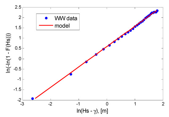
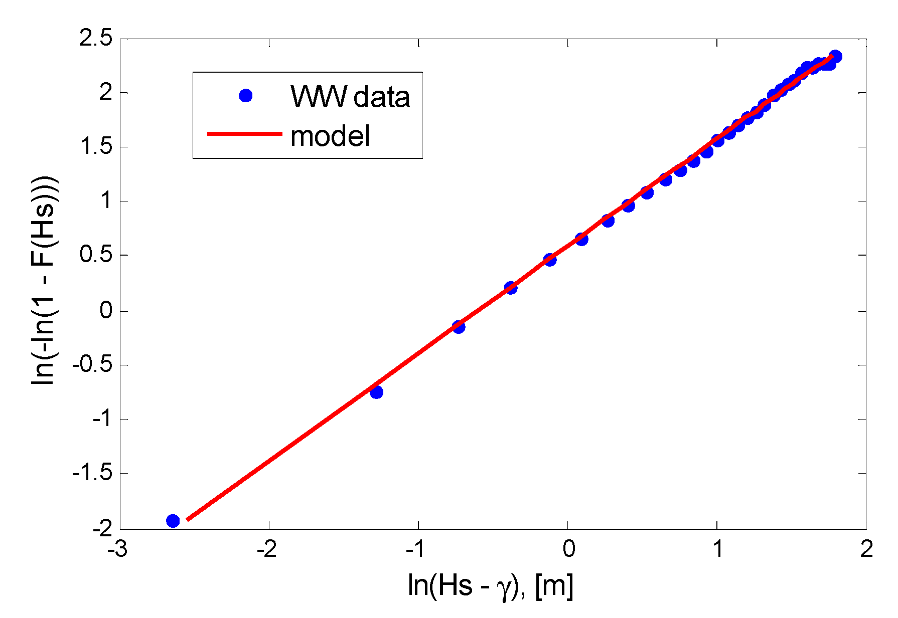
The three-parameter Weibull distribution parameters were fitted for each of the 39 location, for data merged according to the regional subdivision and for the all location merged, i.e., the entire Adriatic Sea. An example fitting on a linearized scale, as per Equation (5), is presented in Figure 6 for location 9, where the maximum Hs was recorded within the database.
Figure 6.
Parameter Weibull parameter fit for marginal distribution of Hs. (E 14.5–N 44.0).
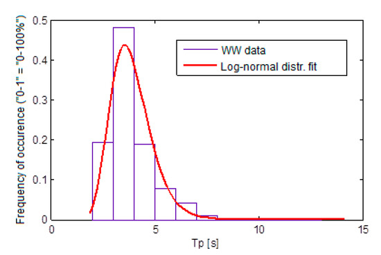
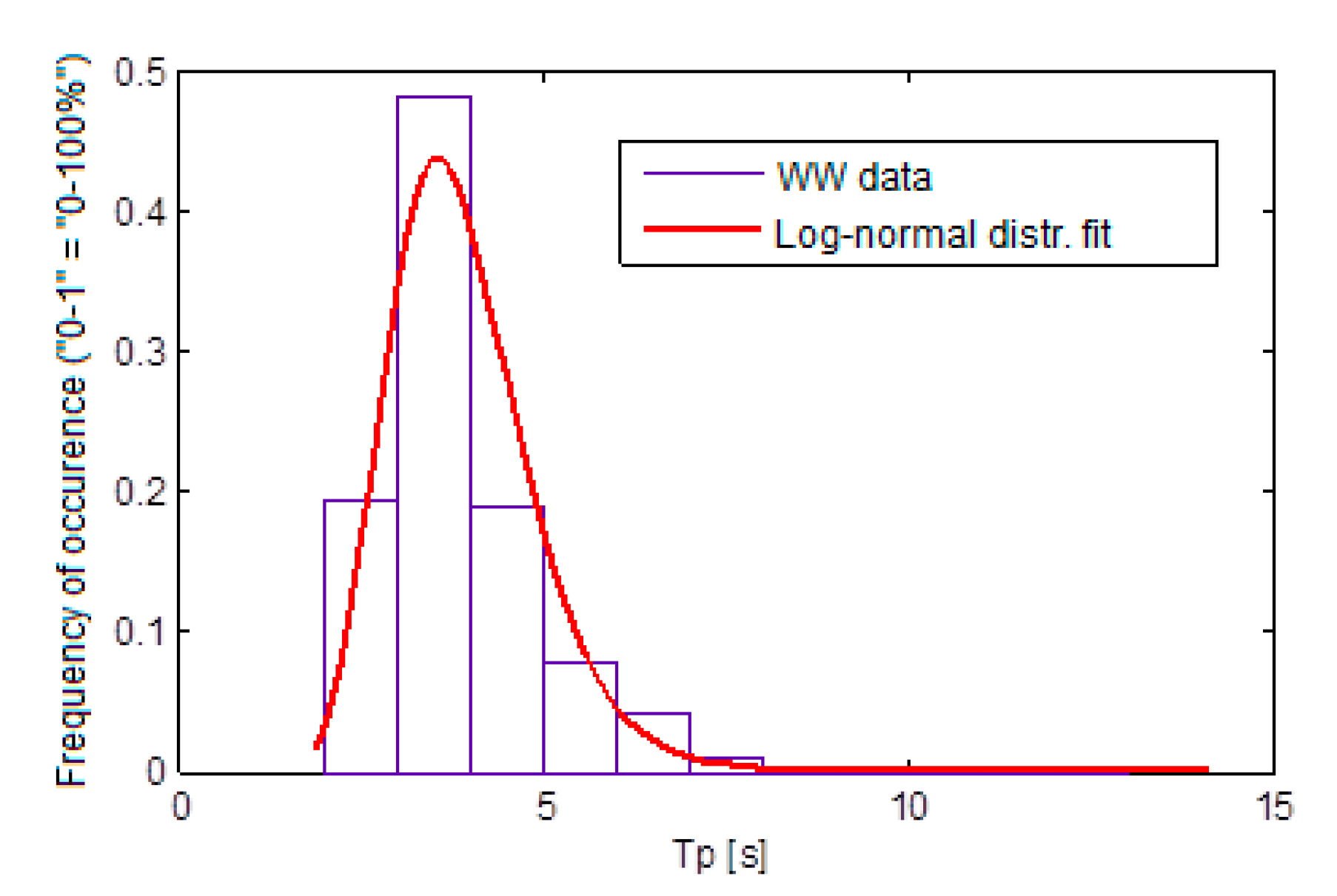
The fit presented in Figure 6 shows an example validation of the model. All 39 location fits were visually inspected, and the calculated coefficient of determination, R2, ranging between R2min = 0.9971 and R2max = 0.9996, confirms that the model is appropriate. Likewise, an example fit is presented in Figure 7 of the log-normal distribution fit for a conditional distribution of peak periods dependent on significant wave height.
Figure 7.
Log-normal conditional distribution fit of Tp on Hs, e.g., Hs = 0.5–1.0 m; E 14.5–N 44.0.
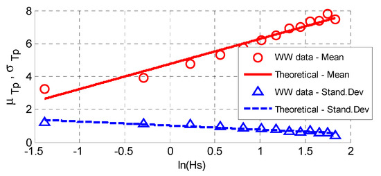
The sea state, Hs and Tp description are completed by determining the mean and the standard deviation values that define the log-normal distribution for the entire bin range of Hs, as presented in Figure 8.
Figure 8.
Mean and standard deviation for calculation of Tp distribution across Hs bin range; E 14.5–N 44.0.
The model parameters for the joint distribution of significant wave height and peak period are finally presented in Table 3 for regions, and Figure 9 and Figure 10 for individual locations.
Table 3.
Model parameters for joint distribution of Hs and Tp. Adriatic regional subdivision.
Figure 9.
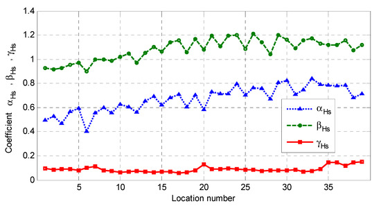
Model parameters for marginal distribution of significant wave height per location.
Figure 10.
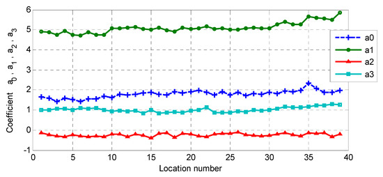
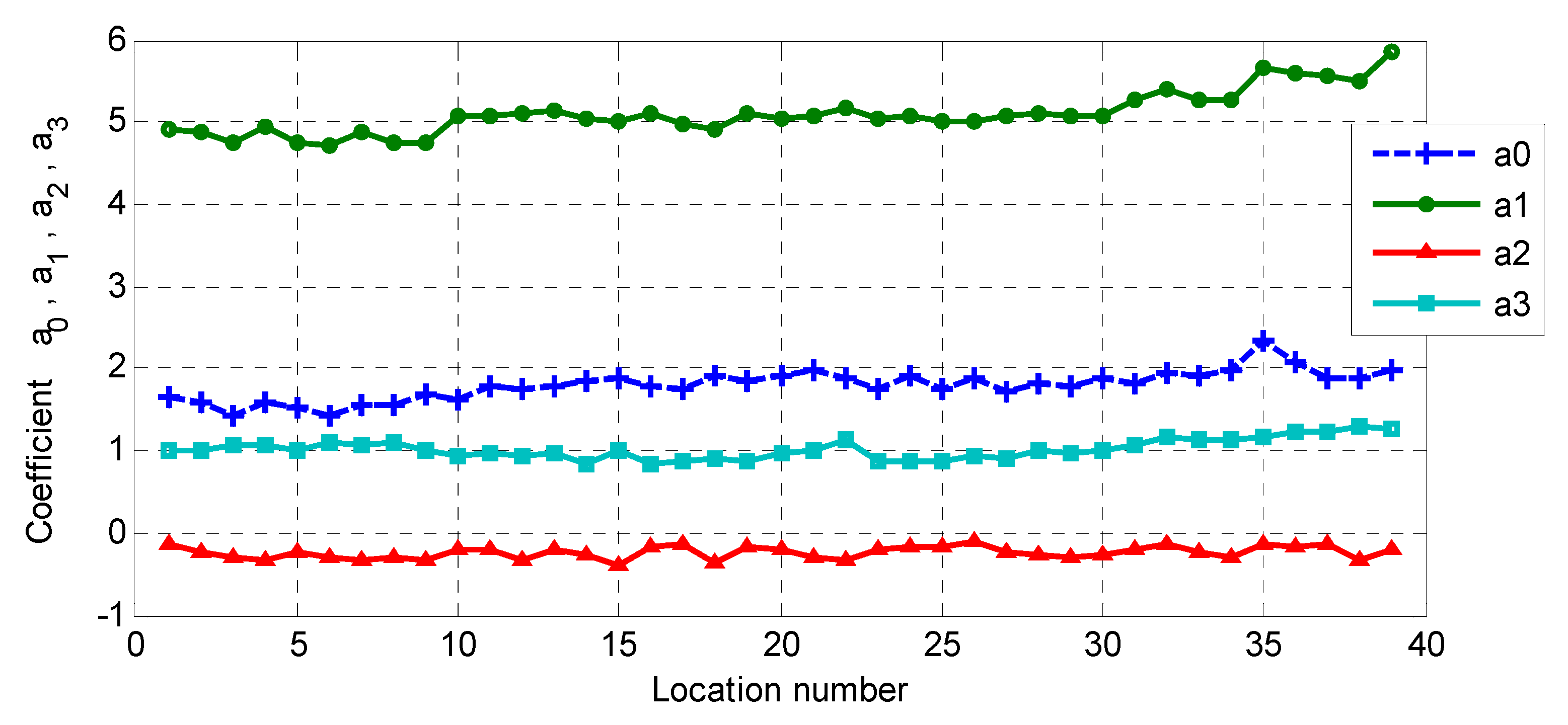
Model parameters for mean and standard deviation across Hs bin range to model log-normal distribution of peak period Tp-per location.
For precision, and to enable repeatability and practical usage, numerical parameters for individual locations are given in Appendix B Table A10.
4.2. Parameters of the Joint Distribution of Wind Speed and Significant Wave Height
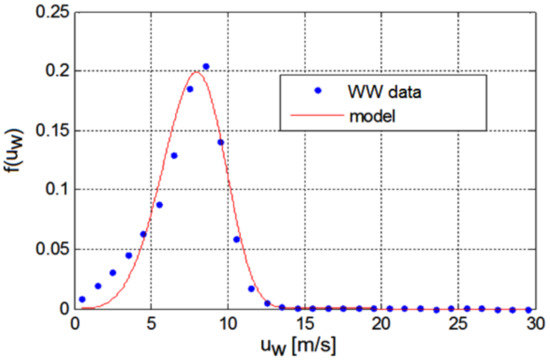
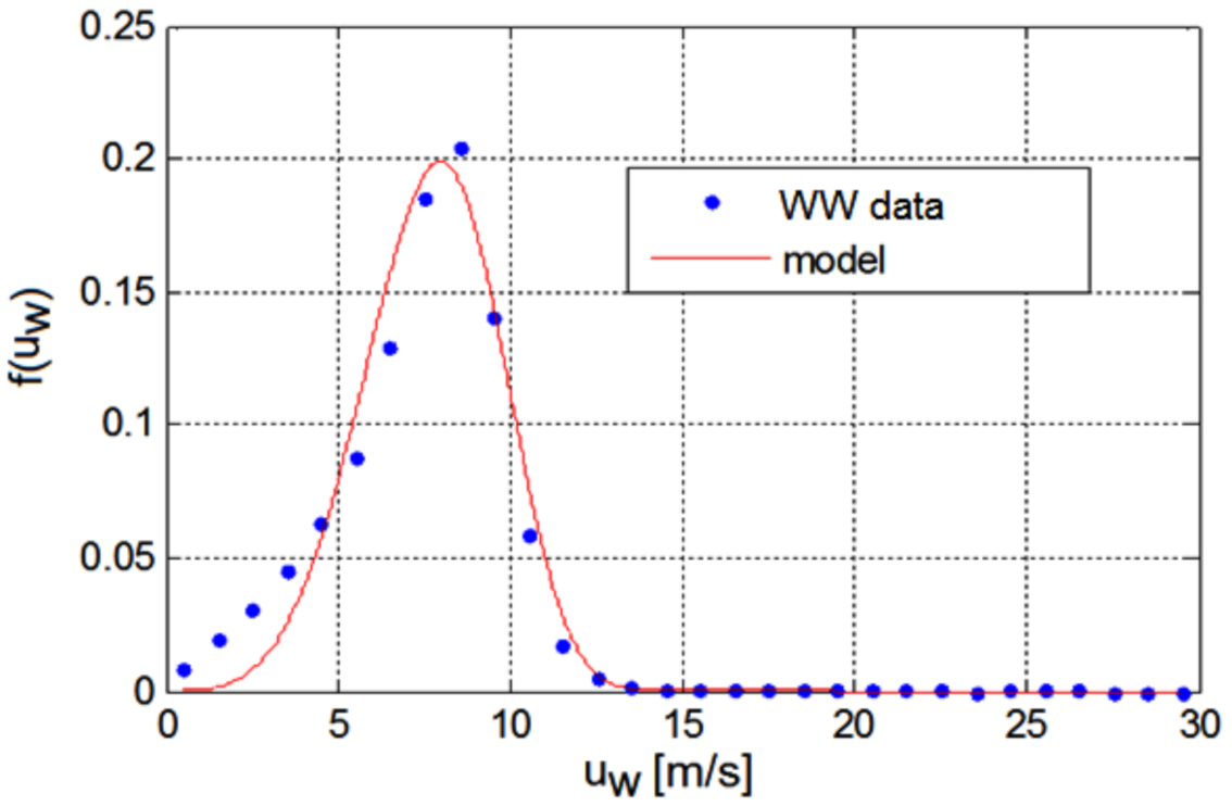
For Hs bins, the theoretical distribution of wind speeds proposed by the model in Equation (11) is derived. The model parameters k and Uc are optimized using the nonlinear least squares method. An example fit of the two-parameter Weibull distribution of wind speed for bin Hs = 2.25–2.5 m for the entire Adriatic is shown in Figure 11.
Figure 11.
Fitting the model to WW data; entire Adriatic; Hs,i = 2.25–2.5 m.
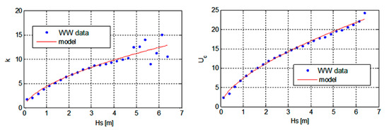
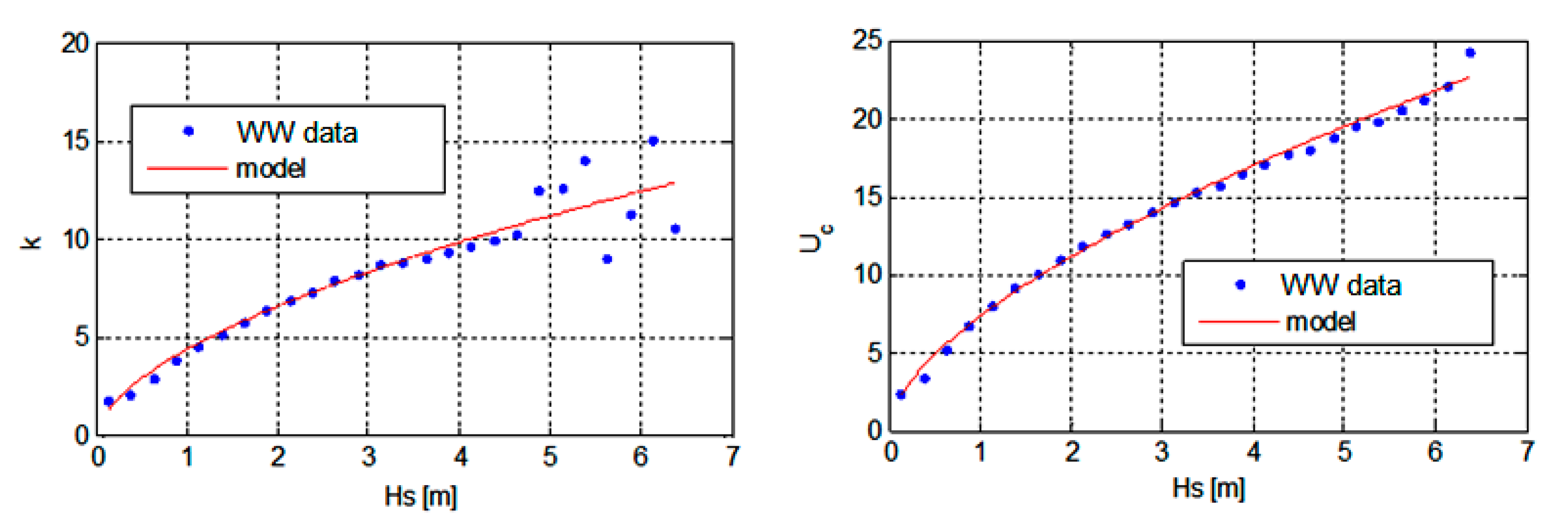
By repeating the same procedure for each Hs,i bin, a model of fit parameters k and Uc is obtained. Their results for the entire Adriatic are presented in Figure 12 as a function of Hs.
Figure 12.
Distribution of k and Uc for Adriatic as a whole.
A data scattering of WW data points for the shape parameter k can be seen for higher Hs values. This feature is even more pronounced having a more detailed look for certain locations and is due to small amount of data at high Hs. Poor agreement of the statistical model at higher values also has a negative effect on poorer agreement of the model with data at lower values. It was found that more than 99.5% of the recorded data are usually below significant wave height of 3.25–3.75 m. In order to achieve a better agreement data corresponding to the highest 0.5% Hs were discarded, both for individual locations analysis and grouped data, having in mind that such filtering makes the model acceptable for fatigue or seakeeping considerations of offshore structures but not for the extreme value analysis.
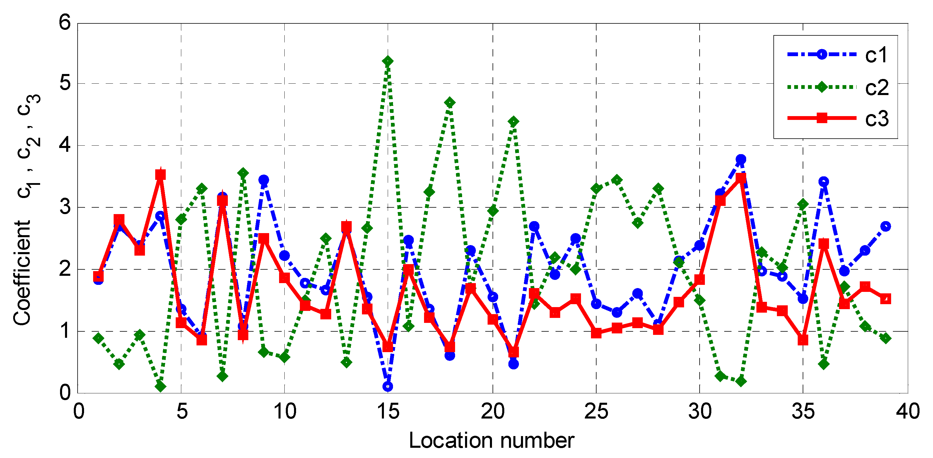
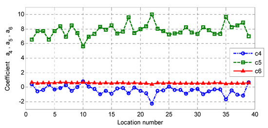
The model parameters for the joint distribution of wind speed and significant wave height are finally presented in Table 4 for regions, and Figure 13 and Figure 14 for individual locations.
Table 4.
Model parameters for joint distribution of Hs and u_w. Adriatic regional subdivision.
Figure 13.
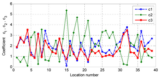
Model parameters c1–c3 for description of the joint distribution of uw and Hs per location.
Figure 14.
Model parameters c4–c6 for description of the joint distribution of uw and Hs per location.
For precision, and to enable repeatability and practical use, parameters for individual locations are given in Appendix B-Table A11.
4.3. Extreme Wave Heights for Different Return Periods
Once the three-parameter Weibull distribution parameters were evaluated (Table 3), determining a theoretical significant wave height probability of occurrence, an extreme Hs value prediction was possible for return periods longer than the initial database by extrapolating the distribution “upper tail” to an appropriate probability of occurrence (Equations (13) and (14)). Most probable extreme significant wave heights for 20-, 50- and 100-year return periods, according to regional subdivision, are presented in Table 5.
Table 5.
Most probable extreme significant wave height for 20-, 50- and 100-year return periods.
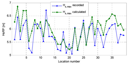
The difference between Hs,max_recorded, the recorded maximum within the WW database and Hs,max_calculated, the most probable theoretical extreme for the exact same return period as the database, per location, is presented in Figure 15.
Figure 15.
Hs comparison, per location, of most probable theoretical extreme and recorded maximum within WW database (duration 23.5 year).
The average difference between Hs,max_recorded and Hs,max_calculated is 4.1% in average across all locations with a standard deviation of 4.7%, i.e., Hs,max_calculated overestimates Hs,max_recorded by 0.23 m in average with a standard deviation of 0.27 m.
For precision, and to enable repeatability and practical use, parameters for individual locations are given in Appendix B-Table A12.
5. Discussion
The results presented in Section 4 provide parameters for a systematic theoretical model of wind and wave statistics for the Adriatic Sea. The distributions are fitted to the data from the WorldWaves database for the period 1992–2016. As such, the results are limited with precision and accuracy of the underlying database. Each data-acquisition technique or modelling approach has limitations but the used dataset currently represent the state-of-the-art by combining a third-generation numerical model hindcast, that provides the systematic character in space and time, with the available satellite altimetry measurements. If a specific random location would be of interest between the analyzed location, four-point interpolation can be used. As for the near-shore region, winds and consequent waves in the Adriatic are highly locally influenced by surrounding land topography, i.e., mountains and islands; thus, results should be extrapolated in those regions with care or used only as boundary conditions for site specific studies.
The applied three-parameter Weibull and log-normal distributions, used for the CMA approach for joint distribution of significant wave height and peak period, showed excellent agreement with the data (e.g., Figure 6 and Figure 7). The upper tail of the fit, essential for extremes evaluation, is always sensitive to fewer data records of high sea states. It thus caries a greater uncertainty also subject to distribution model choice/data preparation and parameter-fitting technique [17,30]. The applied method however remains a common choice and recommendation by classification societies guidelines [2]. The shape and scale parameters in Figure 9 of the three-parameter Weibull distribution show a slight increasing linear trend going towards higher location numbers, i.e., towards the south of the Adriatic. The coefficients for Tp distribution modelling across the Hs range, shown in Figure 10, show almost constant values and could be used as such. On the other hand, the adequacy of the chosen linear model for the mean value parameters across the Hs range, as given in Equations (9) and (10) and presented in Figure 8, exhibits a slight non-linear trend and considering a higher order model could be beneficial.
As for the wind speed to significant wave height fit it should be noted that the highest 0.5% of data were filtered out due to high scatter (Figure 12) to improve fit quality but this makes the model less appropriate for possible upper tail extremes extrapolation. The shape scale parameter Uc shows greater fit confidence than the shape parameter k across the Hs range (Figure 12).
In general, the best accuracy is always expected by applying location or region-specific parameters without generalization as their fit parameters were optimized simultaneously.
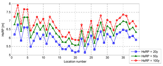
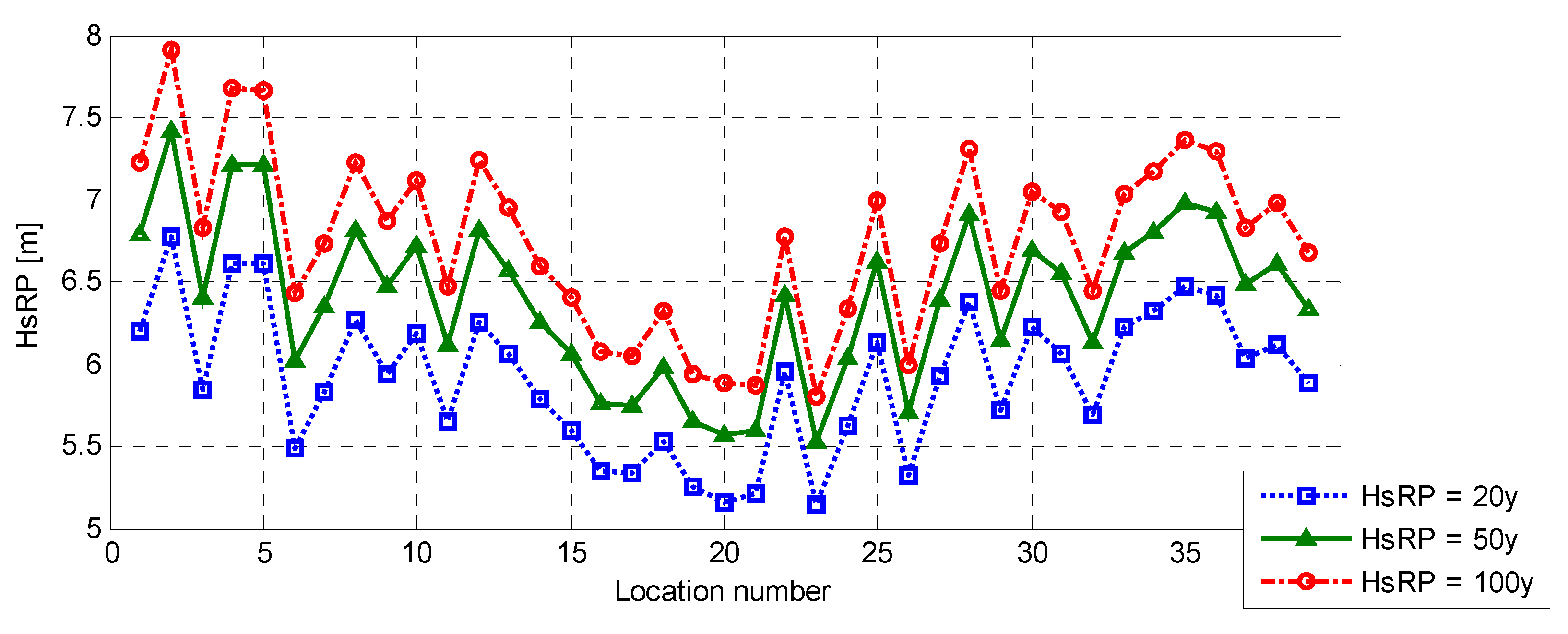
Extremes evaluation as presented in Figure 16, noting the location regional subdivision (North, 1–9; Central, 10–22; South, 23–39), show that highest extremes can be expected in North and South Adriatic and smaller in the Central Adriatic with several locations (20, 21, 22) in its southeast that are closest to South Adriatic and exposed to SE wind (jugo/scirocco) show high extremes as well. The highest recorded significant wave height within the WW database reads 6.72 m (location 9) and the comparable, theoretical, most probable 20-year calculated on merged data for the entire Adriatic reads 5.94 m, thus being un-conservative and highlighting issues of generalization.
Figure 16.
Most probable extreme significant wave height for RP = 20, 50 and 100 y per location.
6. Conclusions
The paper analyzed the wind and wave WorldWaves database (1992–2016), which is an assimilation of numerical hindcast and satellite altimetry wave measurements for a specific wind–wave climate region in the Adriatic Sea. The Adriatic Sea is seeing increasing commercial activity and is a fragile ecological system due to its relatively small area and being a semi-enclosed basin deserving thus an in-detail look. Based on the WW database the models were developed: joint distribution of significant wave height and peak period; extreme significant wave height for long return periods; joint distribution of wind speed and wave height. The model parameters and the extremes are presented for each of the 39 uniformly spaced locations (0.5° × 0.5° lat./long.) across the offshore Adriatic, divided in three regions (North, Central and South Adriatic) and for the entire Adriatic Sea as a whole (all location data merged together). The model parameters, as well as the extremes, can be found presented in paper main body, for the three regions and the Adriatic as a whole, either as tabulated numerical values or graphically. Locations specific results are, for brevity, only graphically presented in paper main body and the numerical tabulated data are provided in the Appendix.
The presented models (Section 3) and optimized model parameters (Section 4/Appendix) provide a complete description of main wind and wave value statistics. Such data can be useful for the design, risk-based operation planning, lifetime extension and maintenance of new and existing seagoing vessels and offshore installations in the Adriatic Sea.
Author Contributions
J.P. provided conceptualization, methodology and supervision; and M.K. executed the formal analysis, investigation and writing. All authors have read and agreed to the published version of the manuscript.
Funding
This work was supported by the Croatian Science Foundation, under the project MODUS lP-2019-04-2085, and the Faculty of Maritime Studies–University of Split, under the project VIF-2674./2017.
Institutional Review Board Statement
Not applicable.
Informed Consent Statement
Not applicable.
Data Availability Statement
The data presented in this study are available within the article, mainly in Appendix A & Appendix B. Restrictions apply to the availability of the underlying WorldWaves database that is the property of Fugro OCEANOR [www.fugro.com; www.oceanor.info, accessed on 5 May 2021].
Acknowledgments
The WorldWaves database is provided by Fugro OCEANOR. The presented work was derived from MK’s doctoral thesis, “Modelling of wind-generated waves in the Adriatic Sea for applications in naval architecture and maritime transportation” (in Croatian), under the mentorship of JP.
Conflicts of Interest
The authors declare no conflict of interest.
Appendix A
Table A1.
Location numbering and coordinates with regional subdivision.
Table A2.
Wind and wave parameters available for each location in in the WW database.
Table A3.
Maximum recoded wave heights, Hs, per location with accompanying parameters. Maximum marked in red.
Sea state tables:
Table A4.
Sea table for North Adriatic region (locations 1–9).
Table A5.
Sea table for Central Adriatic region (locations 10–22).
Table A6.
Sea table for South Adriatic region (locations 22–39).
Wave roses:
Figure A1.
Wave roses for all sea states: (a) South Adriatic, (b) Central Adriatic and (c) North Adriatic.
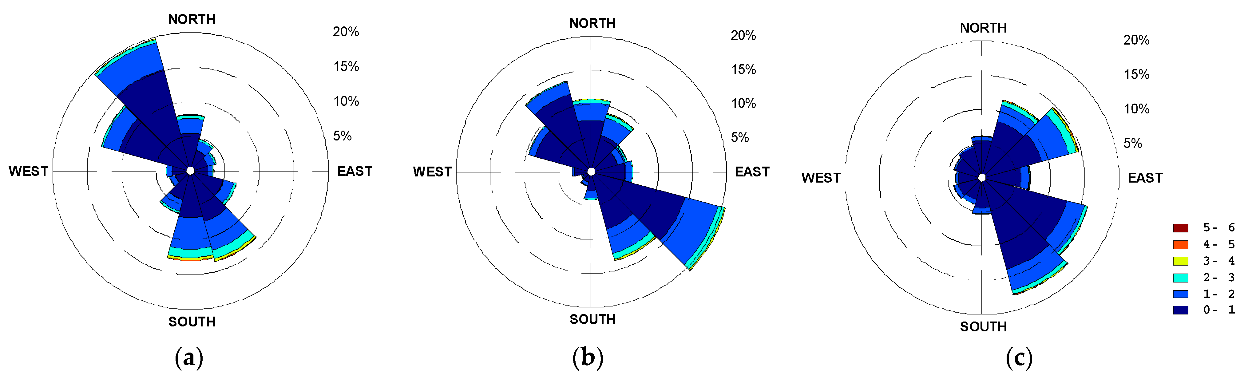
Figure A2.
Wave roses with Hs > 2.5 m: (a) South Adriatic, (b) Central Adriatic and (c) North Adriatic
Wind speed to significant wave height simultaneous occurrence tables:
Table A7.
Wind speed with significant wave height for North Adriatic region (locations 1–9).
Table A8.
Wind speed with significant wave height for Central Adriatic region (locations 10–22).
Table A9.
Wind speed with significant wave height for South Adriatic region (locations 22–39).
Appendix B
Table A10.
Model parameters for joint distribution of Hs and Tp per location.
Table A11.
Model parameters for joint distribution of uw and Hs per location.
Table A12.
Most probable extreme significant wave heights, HsRP (m), for various return periods.
References
- Bitner-Gregersen, E.M.; Dong, S.; Fu, T.; Ma, N.; Maisondieu, C.; Miyake, R.; Rychlik, I. Sea state conditions for marine structures’ analysis and model tests. Ocean Eng. 2016, 119, 309–322. [Google Scholar] [CrossRef] [Scilit]
- Det Norske Veritas. Recommended Practice DNV-Rp-C-205, Environmental Conditions and Environmental Loads. 2019. Available online: www.dnv.com (accessed on 5 May 2021).
- Liščić, B.; Senjanović, I.; Čorić, V.; Kozmar, H.; Tomić, M.; Hadžić, N. Offshore Wind Power Plant in the Adriatic Sea: An Opportunity for the Croatian Economy. Trans. Marit. Sci. 2014, 3, 103–110. [Google Scholar] [CrossRef] [Scilit]
- Det Norske Veritas. Classification Notes No. 30.7: Fatigue Assessment of Ship Structures; 2014. Available online: www.dnv.com (accessed on 5 May 2021).
- Parunov, J.; Rudan, S.; Ćorak, M. Ultimate hull-girder-strength-based reliability of a double-hull oil tanker after collision in the Adriatic Sea. Ships Offshore Struct. 2017, 12 (Suppl. S1), S55–S67. [Google Scholar] [CrossRef] [Scilit]
- Senjanović, I.; Fan, Y. Nonlinear oscillations of quadratic nonlinear systems and its application to mooring analysis. Int. Shipbuild. Prog. 1994, 41, 149–177. [Google Scholar]
- Barbariol, F.; Benetazzo, A.; Carniel, S.; Sclavo, M. Improving the assessment of wave energy resources by means of coupled wave-ocean numerical modelling. Renew. Energy 2013, 60, 462–471. [Google Scholar] [CrossRef] [Scilit]
- Liberti, L.; Carillo, A.; Sannino, G. Wave energy resource assessment in the Mediterranean, the Italian perspective. Renew. Energy 2013, 50, 938–949. [Google Scholar] [CrossRef] [Scilit]
- Ljulj, A.; Slapničar, V. Seakeeping Performance of a New Coastal Patrol Ship for the Croatian Navy. J. Mar. Sci. Eng. 2020, 8, 518. [Google Scholar] [CrossRef] [Scilit]
- Senjanović, I.; Parunov, J.; Ciprić, G. Safety analysis of ship rolling in rough sea. Chaos Solitons Fractals 1997, 8, 659–680. [Google Scholar] [CrossRef] [Scilit]
- Čorić, V.; Ćatipović, I.; Slapničar, V. Floating crane response in sea waves. Brodogradnja 2014, 65, 111–202. [Google Scholar]
- Hydrographic Institute of Republic of Croatia. In Atlas of the Climatology of the Adriatic Sea; HHI: Split, Croatia, 1979. (In Croatian)
- Parunov, J.; Ćorak, M.; Pensa, M. Wave height statistics for seakeeping assessment of ships in the Adriatic Sea. Ocean. Eng. 2011, 38, 1323–1330. [Google Scholar] [CrossRef] [Scilit]
- Soares, C.G. Assessment of the uncertainty in visual observations of wave height. Ocean Eng. 1986, 13, 37–56. [Google Scholar] [CrossRef] [Scilit]
- Bencivenga, M.; Nardone, G.; Ruggiero, F.; Calore, D. The Italian data buoy network (RON). Adv. Fluid Mech. Ix 2012, 74, 305. [Google Scholar]
- Pomaro, A.; Cavaleri, L.; Papa, A.; Lionello, P. 39 years of directional wave recorded data and relative problems, climatological implications and use. Sci. Data 2018, 5, 180139. [Google Scholar] [CrossRef] [Scilit] [PubMed]
- Katalinić, M.; Parunov, J. Wave statistics in the Adriatic Sea based on 24 years of satellite measurements. Ocean Eng. 2018, 158, 378–388. [Google Scholar] [CrossRef] [Scilit]
- Katalinić, M.; Parunov, J. Uncertainties of Estimating Extreme Significant Wave Height for Engineering Applications Depending on the Approach and Fitting Technique—Adriatic Sea Case Study. J. Mar. Sci. Eng. 2020, 8, 259. [Google Scholar] [CrossRef] [Scilit]
- Barstow, S.; Mørk, G.; Lønseth, L.; Mathisen, J.P. WorldWaves wave energy resource assessments from the deep ocean to the coast. J. Energy Power Eng. 2011, 5, 730–742. [Google Scholar]
- Barstow, S.F.; Mo̸rk, G.; Lo̸nseth, L.; Schjo̸lberg, P.; Machado, U.; Athanassoulis, G.; Belibassakis, K.; Gerostathis, T.; Stefanakos, C.; Spaan, G. WORLDWAVES: High quality coastal and offshore wave data within minutes for any global site. In Proceedings of the 22nd International Conference on Offshore Mechanics and Arctic Engineering, Cancun, Mexico, 8–13 June 2003; Volume 3, pp. 633–642. [Google Scholar]
- Romeiser, R. Global validation of the wave model WAM over a one-year period using Geosat wave height data. J. Geophys. Res. Space Phys. 1993, 98, 4713–4726. [Google Scholar] [CrossRef] [Scilit]
- Heimbach, P.; Hasselmann, S. Statistical analysis and intercomparison of WAM model data with global ERS-1 SAR wave mode spectral retrievals over 3 years. J. Geophys. Res. Space Phys. 1998, 103, 7931–7977. [Google Scholar] [CrossRef] [Scilit]
- Tabain, T. Standard wind wave spectrum for the Adriatic Sea revisited (1977-1997). Brodogradnja 1997, 45, 303–313. [Google Scholar]
- Bitner-Gregersen, E.M.; Haver, S. Joint long term description of environmental parameters for structural response calculation. In Proceedings of the 2nd International Workshop on Wave Hindcasting and Forecasting, Vancouver, BC, Canada, 25 April 1989; pp. 25–28. [Google Scholar]
- Bitner-Gregersen, E.M. Joint long term models of met-ocean parameters. In CENTEC Anniversary Book; Soares, C.G., Garbatov, Y., Fonseca, N., Texeira, A.P., Blakema, A.A., Eds.; Taylor and Francis: London, UK, 2012. [Google Scholar]
- Parunov, J.; Senjanovic, I. Methods for long-term prediction of extreme sea states. Brodogradnja 2000, 48, 131–138. (In Croatian) [Google Scholar]
- Nordenström, N. A method to predict long-term distributions of waves and wave-induced motions and loads on ships and other floating structures. In Classification and Registry of Shipping, Report 81; Det Norske Veritas: Oslo, Norway, 1973. [Google Scholar]
- MATLAB. Fitting a Univariate Distribution Using Cumulative Probabilities—A Threshold Parameter Example. Available online: https://www.mathworks.com/help/stats/fitting-a-univariate-distribution-using-cumulative-probabilities.html (accessed on 5 May 2021).
- Mathisen, J.; Bitner-Gregersen, E. Joint distributions for significant wave height and wave zero-up-crossing period. Appl. Ocean Res. 1990, 12, 93–103. [Google Scholar] [CrossRef] [Scilit]
- Mauro, F.; Braidotti, L.; La Monaca, U.; Nabergoj, R. Extreme loads determination on complex slender structures. Int. Shipbuild. Prog. 2019, 66, 57–76. [Google Scholar] [CrossRef] [Scilit]

Publisher’s Note: MDPI stays neutral with regard to jurisdictional claims in published maps and institutional affiliations. |
© 2021 by the authors. Licensee MDPI, Basel, Switzerland. This article is an open access article distributed under the terms and conditions of the Creative Commons Attribution (CC BY) license (https://creativecommons.org/licenses/by/4.0/).