Wind Energy Ships: Global Analysis of Operability

Abstract

Most offshore wind farms are bottom-fixed at sites with less than 50 m of water depth. For deeper waters, floating platforms are economically viable and, for many countries that have steep continental shelves, this is the only option for developing offshore wind farms. If wind energy is being harvested far offshore in deep waters (more than 200 m depth and hundreds of km from the coast), one possible alternative is the use of Floating Production and Storage (FPS) sailing ships that navigate through the ocean using wind force and utilize part of the harvested wind power to produce and store fuel. These ships are called “energy ships”. The objective of this paper is to carry out a qualitative determination of the global marine areas suitable for the operation of energy ships. To that purpose, wind and wave ship operation ranges have been defined and global databases of wind and waves have been used to obtain statistics of operational parameters. From the global analysis carried out the most promising areas and seasons for energy ship operation have been identified and qualified in terms of the aforementioned operational parameters.

1. Introduction

Offshore wind has been sustaining an accelerated development during the last decades. With a total net installed capacity of 189 GW in 2018, (19 GW offshore), wind energy remains the second largest form of power generation capacity in Europe, set to overtake gas installations in 2019 [1].

Globally, industry installed a record 5.652 MW of offshore wind capacity in 2018. China alone installed 2.652 GW of new capacity and European countries 2.7 GW. By the end of 2018, cumulative global offshore wind installed capacity grew to 22.592 GW from 176 operating projects [2].

Most of the offshore wind farms are bottom–fixed at less than 50 m of water depth. For deeper waters, floating platforms are economically competitive and for many countries that have steep continental selves this is the only option for developing offshore wind farms. According to [2] there are currently eight floating offshore wind projects installed around the world representing 46 MW of capacity. Five projects (37 MW) are installed in Europe and three (9 MW) are in Asia. There are an additional 14 projects representing approximately 200 MW that are currently under construction or have achieved either financial close or regulatory approval. Two projects (488 MW) have advanced to the permitting phase of development, and another 14 are in the early planning stages (4162 MW).

According to [3], the global offshore wind technical potential available nearshore (distance to the shore < 90 km) and in intermediate waters (water depth < 200 m) is around 180,000 TWh/y which is less than the expected demand in 2050 (240,000 TWh/y) [4]. This means that if floating offshore wind power is intended to cover the world energy demand, it must move deeper and further away from the coast. Moving floating wind offshore create new challenges; first, grid connection increases linearly with increasing distance to the shore [5]. Second, moorings and anchors (including installation) share of the operational expense become increasingly dominant, for example, in present floating offshore wind projects they account for around 20% of capital expenditure [6].

In [3] it is estimated that the global onshore wind energy resource in the lower atmosphere is around 1.1 × 10⁶ TWh/y. Taking into account that the oceans cover 2/3 of the Earth’s surface, a lower estimate for the lower atmosphere offshore wind resource of 2.2 × 10⁶ TWh/y is made in [7]. This number is around 12 times the nearshore resource and nine times the 2050 estimated world energy demand.

If wind energy is being to be harvested far offshore in deep waters (more than 200 m depth and hundreds of km from the coast), there are two possible alternatives (1) anchored floating wind farms with anchored floating production storage and offloading vessels (FPSO) to transform the electric energy into a hydrogen-rich fuel that is stored in the vessel until being unloaded to a tanker and shipped to the shore, and (2) floating production and storage (FPS) sailing ships that navigate through the ocean using the wind force and utilize part of the harvested wind power to produce and store the fuel. Once the ship tanks are full, they can be unloaded to a supply vessel at sea or navigate to a convenience port to unload the fuel and return to the wind harvesting area to start again the cycle.

In [8], the first proposals to assess wind energy in deep waters, some US patents and first approaches for using conventional ships to harvest wind energy in the open ocean are described.

To this respect, References [9,10,11,12] proposed to use a very large floating structure (VLFS) supporting several wind turbines, sails, and thrusters and capable to navigate looking for routes that maximize energy input, avoiding storm areas. They concluded that the VLFS navigation capabilities improved the energy yield and load factor in comparison with the fixed one. In [7] these ships are called “energy ships”, a term derived from the renewable energy ships that are being currently developed to save fuel taking advantage of renewable energy sources as wind or sun [13]. In [7,14,15] a comprehensive review of possible energy ships configurations was presented.

One of the most promising configuration of energy ships propose the use of sails for ship propulsion and hydrokinetic turbines for energy generation. This energy is used for the ship operation and hydrogen-rich fuel production and storage. In this respect, Reference [16] analyzed, numerically and in laboratory models, ships with sails, turbines, and generators with 1.5 MW electrical power (prototype) output. Additionally, a discussion on the feasibility of sea water electrolysis for hydrogen and oxygen production was included. In [17] it was proposed and modelled numerically the use cargo ships with Flettner rotors for propulsion, photovoltaic generators, wind turbines, and dual model propellers to produce energy for the auxiliary systems for the Flettner rotors as well as for batteries to balance the energy production in realistic weather conditions. Results showed that feasible navigation speeds were achievable in route, but the negative energy balance limited energy production. In [18] a comprehensive review of previous proposals is given and the performance of autonomous sailing ships with hydrokinetic turbines to produce energy that can be either stored in batteries or to produce hydrogen via water electrolysis is analyzed. Produced hydrogen is compressed and stored in the ship. The paper concludes with a discussion of the potential of this concept to achieve the IPCC-mandated requirement of reducing the global CO2 emissions. Recently, Tokyo-Mitsui O.S.K. Lines, Ltd. (Tokyo, Japan) announced the creation of a joined corporate-academic partnership in a zero-emission initiative called Wind Hunter Project [19], seeking new applications for hydrogen fuel and wind power. The Wind Hunter Project seeks to combine wind propulsion sailing technology and wind energy converted to generate a stable supply of hydrogen. A recent book [20] show that at present, there is technology to build and operate autonomous sailing ships equipped with hydrokinetic turbines and electrolyzers that could operate in high-wind ocean areas. It also introduces 12 specific technologies that could enable the green energy ship concept.

The main advantages of energy ships over stationary deep water FPSO farms are two-fold: First, the energy ship could sail to the areas where the wind and wave characteristics are appropriate, depending on location and season to optimize power production. Second, the energy ship may avoid areas with extreme wind and waves, something that would put deepwater wind farms in survival mode and provoke the detachment of the FPSO from the mooring to take evasive survival strategies. The main disadvantages of energy ships are that they need part of the harvested wind energy to propel the ship and, in some cases, a secondary conversion of the ship kinetic energy into electricity, adding complexity to the system and reducing the overall performance.

Until now the global analysis of wind energy resources has been assessed using hindcast or measured databases with the objective of determining the wind resource statistical distribution both in space and time [21]. In this paper, global reanalysis databases of wind and waves are used to analyze the suitability of ocean areas for the deployment of energy ships in terms of operational conditions associated to wind speed and wave height.

Within the frame of the 2016 SODERCAN (Society for Cantabria Regional Development) program dedicated to R&D Projects in Marine Renewable Energies, a consortium of four entities developed the project Ship 4 Blue (S4B) [22] with the main objective of conduct a feasibility assessment of energy ships equipped with rigid retractable sails to produce, process, and store ammonia and oxygen. The wind power is used to produce the necessary towing force to generate electricity via hydrokinetic turbo-generators attached to the ship hull or towed by the ship.

This paper is a description of the analysis performed to carry out a qualitative determination of the global marine areas suitable for the operation of energy ships and is organized as follows. In Section 2, the global wind and wave databases used in the project are described and a preliminary analysis of wind and waves spatial and temporal variability is presented. Section 3 is dedicated to the description of the wind and waves ship operational ranges. Section 4 deals with the description and analysis of results of global ship operability areas and, finally, Section 5 presents the conclusions of the research performed.

2. Global Wind and Wave Spatial and Temporal Variability

In this section the global reanalysis databases of wind and waves used in the S4B project are described and a descriptive analysis of the spatial and temporal distribution of main statistics is performed.

2.1. Global Wind Database

The Climate Forecast System Reanalysis (CFSR) [23], is a reanalysis product resulting from a joint initiative of the National Centre for Environmental Prediction (NCEP) and the National Centre for Atmospheric Research (NCAR). The reanalysis is a coupled system between atmosphere, ocean, and sea ice designed to produce the best estimation of the state of these domains at a global scale and high resolution. CFSR includes (1) atmosphere-ocean coupling to generate a prediction field each 6 h, (2) an interactive sea ice model and (3) satellite data assimilation. The atmosphere horizontal resolution is around 38 Km (T382) with 64 levels. The ocean resolution is 0.25 degrees in the tropics and more than 0.5 degrees in the rest with 40 levels. The land surface and sea ice models have four and three levels, respectively. For the purpose of this research, the time series of the hourly average of wind speed at 10 m level, V_i and direction, ϕ_i for each wind state “i” have been used.

The CFSR reanalysis provides wind state parameters data from 1979 to 2010 with hourly temporal resolution and 0.5 × 0.5 degrees spatial resolution. From 2011 onwards, CFSR has been continued by the operational model Climate Forecast System Version 2 (CFSV2) [24]. The operational implementation of the full system ensures a continuity of the climate record and provides a valuable up-to-date dataset to study many aspects of predictability on the seasonal and sub-seasonal scales.

2.2. Global Waves Database

The Global Ocean Waves Two database (GOW2) [25] is a wave hindcast based on WaveWatch III (WWIII) version 4.18 [26]. WWIII is a third-generation wave model that solves the spectral wave action density balance equation for the generation and propagation of waves. GOW2 divides the World Ocean in four regular meshes, see Figure 1: the global mesh (0.5 × 0.5 degrees), two regional meshes that cover the Arctic and Antarctic areas (0.25 degrees latitude × 0.5 degrees longitude) and the coastal mesh (0.25 × 0.25 degrees). This coastal mesh includes all the points with water depth below 200 m and a surrounding area of 1.5 degrees. The wave spectra are defined for 24 directions and 32 frequencies that grow non-linearly from 0.0373 Hz to 0.7159 Hz, each frequency being 1.1 times the previous one.

GOW2 database stores hourly sea state parameters, such as zero-order moment wave height, H_mo, mean and peak wave periods, T_m and T_p, respectively, mean wave direction, θ_m, directional spreading, D_spr and mean wave energy flux, F_m. Additionally, more than 40,000 3-h spectra along the World coasts were stored with 0.25 × 0.25 degrees spatial resolution. Comparisons with instrumental data showed a clear improvement with respect to existing global hindcasts, especially in semi-enclosed basins and areas with a complex bathymetry. The effect of tropical cyclones is also well-captured due to the high resolution of wind forcing and the wave model setup.

2.3. Global Analysis of Wind and Wave Variability.

Previously to the global analysis of energy ships operability, a check of the databases information has been carried out in order to have a preliminary look at the global wind and wave spatial and temporal variability. Denoting by “P” at the hourly state parameter (P = V, hourly average wind speed and P = H, hourly significant wave height), the following statistics are calculated:

• P Mean:

$${\mathsf{\mu }}_{\mathrm{P}}=\frac{1}{\mathrm{N}}{\displaystyle \sum }_{\mathrm{j}=1}^{\mathrm{N}}\left(\frac{1}{{\mathrm{M}}_{\mathrm{j}}}{\displaystyle \sum }_{\mathrm{i}=1}^{{\mathrm{M}}_{\mathrm{j}}}{\mathrm{P}}_{\mathrm{i}}\right)=\frac{1}{\mathrm{N}}{\displaystyle \sum }_{\mathrm{j}=1}^{\mathrm{N}}\overline{{\mathrm{P}}_{\mathrm{j}}}$$

(1)

where, in Equation (1), N is the number of years of the database, M_j is the number of hours of year “j” and $\overline{{\mathrm{P}}_{\mathrm{j}}}=\frac{1}{{\mathrm{M}}_{\mathrm{j}}}{{\displaystyle \sum }}_{\mathrm{i}=1}^{{\mathrm{M}}_{\mathrm{j}}}{\mathrm{P}}_{\mathrm{i}}$ is the mean value of P in the year “j”.

• Standard deviation of P:

$${\mathsf{\sigma }}_{\mathrm{P}}=\frac{1}{\mathrm{N}}{\displaystyle \sum }_{\mathrm{J}=1}^{\mathrm{N}}{\left[\frac{1}{{\mathrm{M}}_{\mathrm{j}}-1}{\displaystyle \sum }_{\mathrm{i}=1}^{{\mathrm{M}}_{\mathrm{j}}}{\left({\mathrm{P}}_{\mathrm{i}}{-\mathsf{\mu }}_{\mathrm{P}}\right)}^2\right]}^{1/2}$$

(2)

• Inter-annual standard deviation of the mean P:

$${\mathsf{\sigma }}_{\mathrm{i}\mathrm{P}}={\left(\frac{1}{\mathrm{N}-1}{\displaystyle \sum }_{\mathrm{j}=1}^{\mathrm{N}}{\left(\overline{{\mathrm{P}}_{\mathrm{j}}}{-\mathsf{\mu }}_{\mathrm{P}}\right)}^2\right)}^{1/2}$$

(3)

Figure 2 shows the global distribution of parameters ${\mathsf{\mu }}_{\mathrm{V}}{,\mathsf{\sigma }}_{\mathrm{V}}{,\mathrm{and}\mathsf{\sigma }}_{\mathrm{iV}}$. As can be seen the global distribution of μ_V shows two clear maxima around the polar front belts, more pronounced in the southern hemisphere (SH). Other less pronounced maxima appear in the trade wind belts, more noticeable the one in the Indian Ocean. Local maxima, associated to monsoons or special land-sea features can be seen in the East and South China Seas around Taiwan, in the Indian Sea near the Horn of Africa and in the Caribbean Sea, to the north of Guajira and Paraguaná peninsulas (in the following the Caribbean Spot). These features of global winds have already been reported by other authors [21,27,28].

The global distribution of σ_V shows a clear difference between the polar front and trade wind belts. Polar front winds variability is much higher, reflecting the seasonal variability and the corresponding short-term changes associated to the variations of the storm tracks and intensities. Especially significant is the peak of variability located between Greenland and Iceland in the North Atlantic. In this area, the variation coefficient, σ_V/μ_V is around 50%. In other areas of the polar front belts, the variation coefficient is lower, between 30% and 40%, being higher in the northern hemisphere (NH). In contrast, the trade winds belts show lower variability, with variation coefficients between 25% and 30%. The East China Sea, South China Sea, and the Indian Ocean affected by the Asian monsoon show also medium to high variability as a consequence of the change of wind directions and intensities associated to the monsoons.

The σ_iV is, in general low, showing maxima around the polar fronts, where the wind intensity is higher (being higher in the SH) and around the equatorial calms belt.

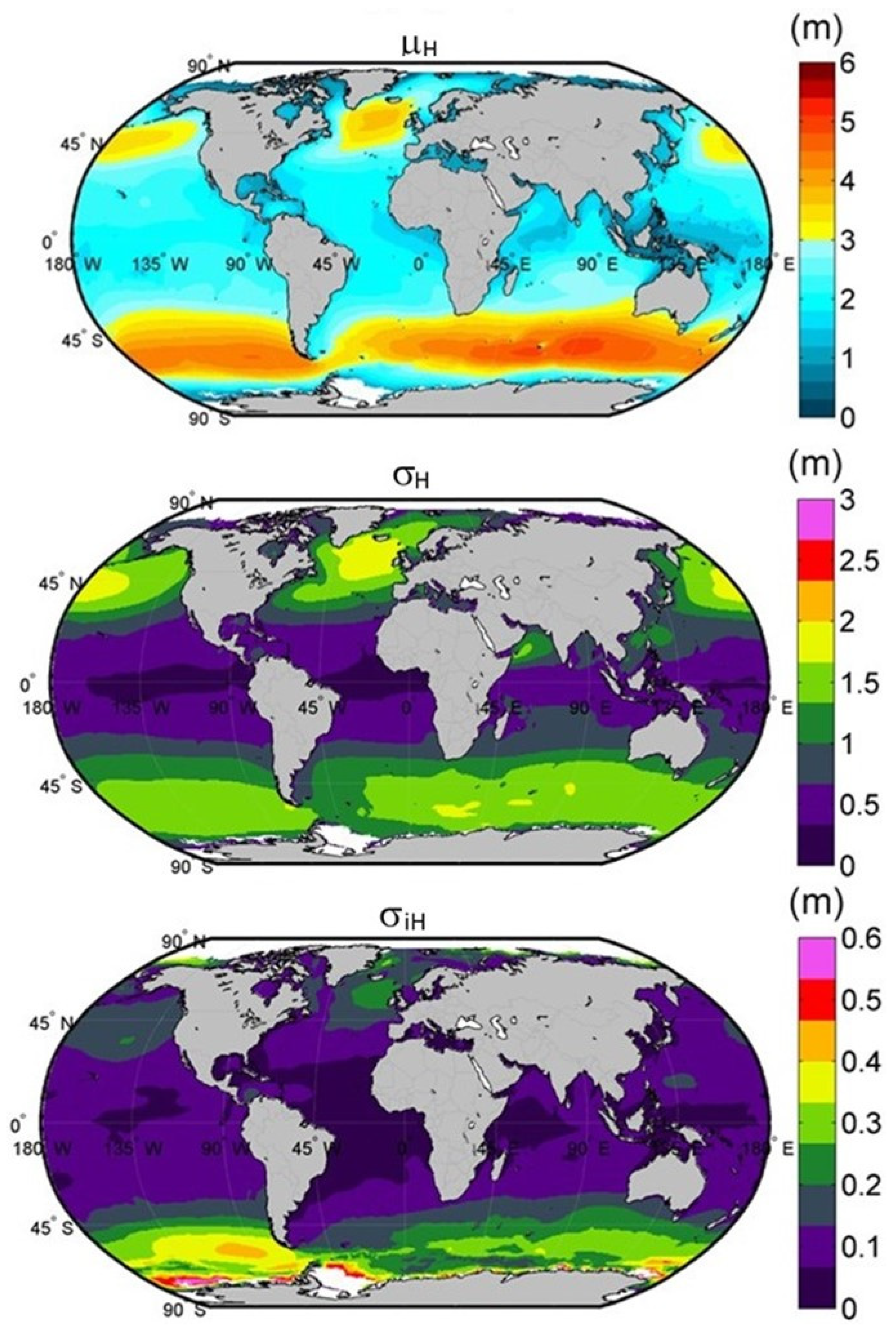
Regarding with the global significant wave height variability, Figure 3 shows the global distribution of parameters ${\mathsf{\mu }}_{\mathrm{H}}{,\mathsf{\sigma }}_{\mathrm{H}}{,\mathrm{and}\mathsf{\sigma }}_{\mathrm{iH}}$. As can be seen in Figure 3, the pattern of μ_H shows the high wind waves associated to the strong winds of the polar front belts. In regards to the wave height variability, again σ_H is highest in the polar front belts with variation coefficients, σ_H/μ_H between 30% and 40%, being the highest in the Northern Pacific with values around 50%. As in the case of the wind velocity, the wave height variability is higher in the NH than in the SH.

The inter-annual variability of the significant wave height, σ_iH, is low in general, being maximum in the polar front belts with variation coefficients between 4% and 10%, being higher in the SH.

3. Wind and Wave Energy Ship Operational Ranges

Sailing energy ships depend on wind for propulsion and energy generation. In the S4B project the sails propel the ship and activate hydrokinetic turbo-generators (attached to the hull or towed) to produce electricity. The operation of sails and turbines will depend on the wind speed, ship velocity and significant wave height. Wind speed determines the ship velocity, power production, and sail integrity, while waves may affect ship navigational capabilities and turbo-generators operation.

Among the S4B research tasks, an economical and financial projection model has been developed to obtain the final production costs in terms of operability variables and ship size and configuration. Using that model, it was found that the lowest LCOE was obtained with the largest of the three reformed bull carrier of tanker sizes analyzed (100, 150, and 300 m length).

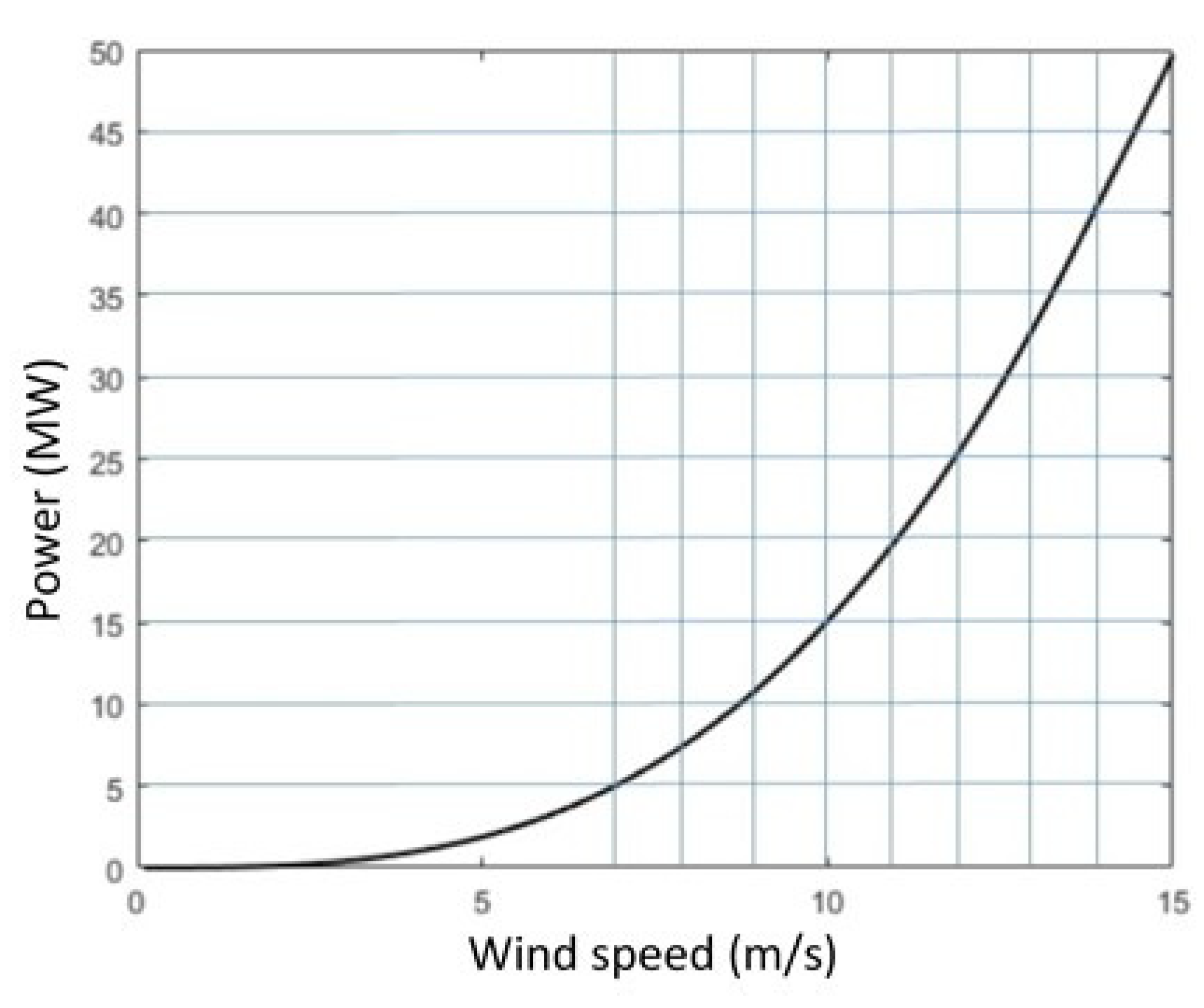
From the analysis carried out, the fully deployed sails could withstand winds up to 20 m/s without compromising their structural integrity, but the nominal wind velocity operation was defined for 15 m/s winds. Part of the wind generated power is used to propel the ship and the rest (towing power) become available to drag the hydrokinetic turbo generators. The ship available towing power in terms of the average wind speed is shown in Figure 4. As can be seen, the available towing power reaches 50 MW for 15 m/s winds. Using that power and assuming a 50% turbo-generator efficiency, the assumed nominal electric power of the generators is 25 MW. The generators cut-in power is established at 2.5 MW for wind speeds of 7 m/s. For wind speeds between 15 and 20 m/s, the ship will produce the nominal power reducing the sail height or modifying the sail pitch angle. The optimum operational range has been established for wind speeds between 10 and 15 m/s.

In terms of wave height, it has been assumed that the ship could navigate with turbo generators producing the nominal power in seas up to 6 m of significant wave height although optimal conditions are those with significant wave height below 4 m.

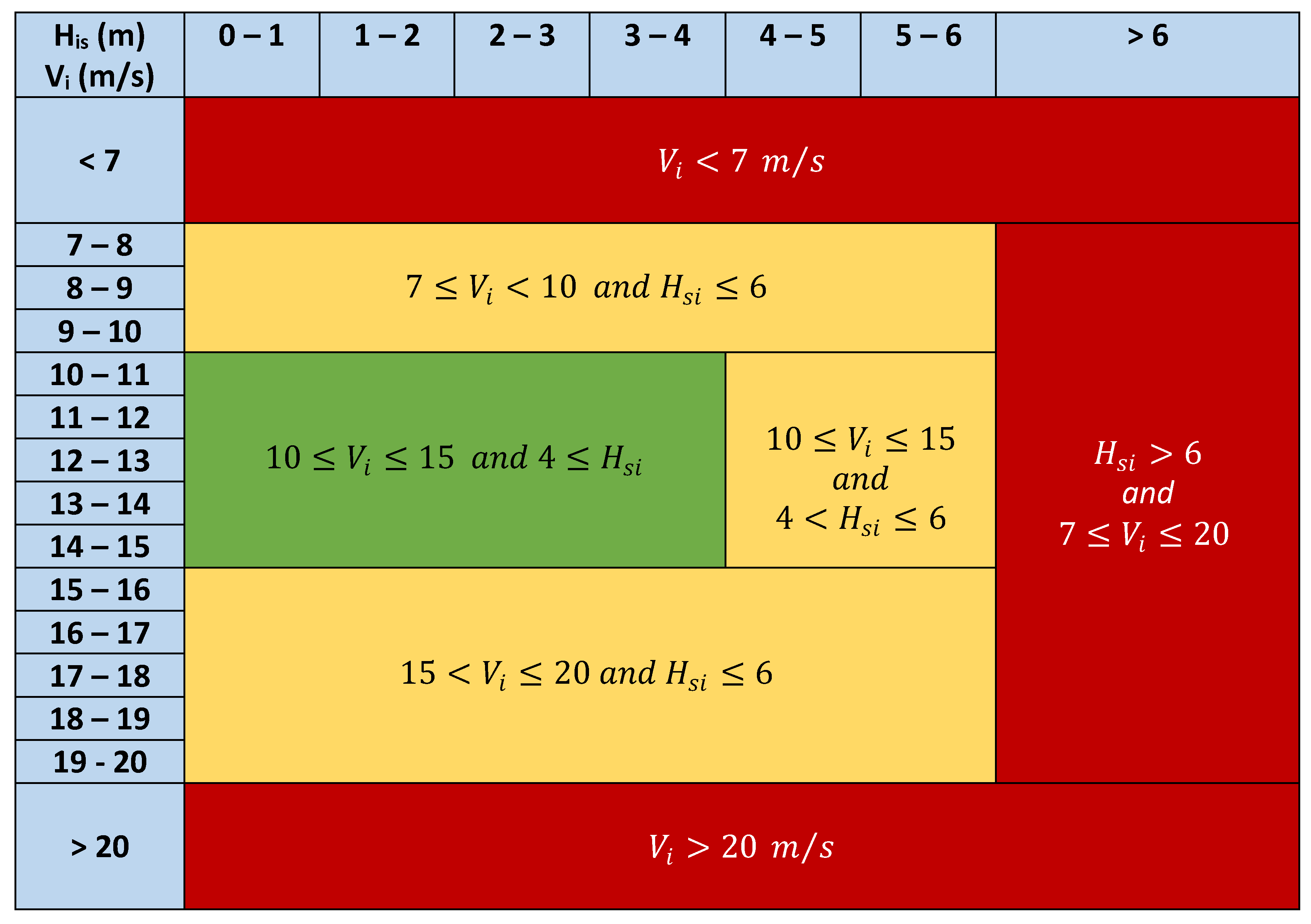
Figure 5 summarizes the sailing operational ranges. The optimal range is indicated in green, the suboptimal in yellow and the non-operative conditions in red. In the following, the operation range that sum up the optimal and suboptimal ranges will be called operability range.

4. Global Analysis of Energy Ship Operability

The global data bases of wind and waves described in Section 2 have been sorted following the ranges of Figure 5, and global statistics maps have been obtained through the calculation the following statistics for each node of the global mesh:

• Annual mean operability, µ₀
• Annual mean optimum operability, µ_p
• Seasonal mean operability, µ_0(Season)
• Seasonal mean optimum operability, µ_p(season)
• Annual mean duration of operability and non-operability intervals, µ_d and µ_dno, respectively.
• Seasonal mean duration of non-operability intervals, µ_dno(Season)

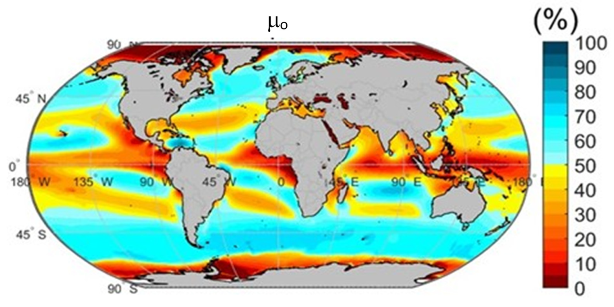
4.1. Global Distribution of the Annual Mean Operability

Figure 6 shows the global distribution of, µ_0. As can be seen there are four great areas having µ₀ over 50%: The polar fronts and the trade winds belts. Additionally, there are other smaller local areas of high µ₀ in the East and South China Seas around Taiwan Island, in the southeast of the Vietnam coast, in the Indian Sea near the Horn of Africa, around Ceylon Island and in the north and south tips of Madagascar Island, associated with monsoons. This results closely follow the distribution of the mean wind velocity, indicating the prevalence of wind over wave conditions on the mean operability of energy ships.

4.1.1. Annual Mean Operability in the Trade Winds Belts

Trade winds are generated by the atmospheric subsidence created by the subtropical high pressures. At surface level, trade winds blow from NE to E in the NH and from SE to E in the SH.

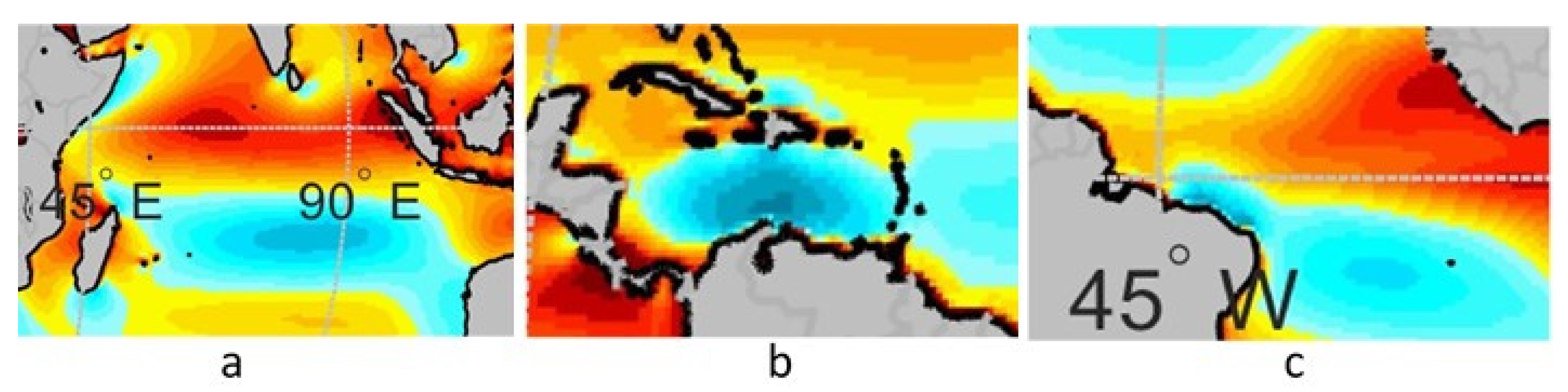
Among the trade winds belts, the following areas have µ₀ over 75%:

The Indian Ocean trade winds, in a strip of about 22 degrees longitude and 4 degrees latitude, centered in 86° E 15° S, see zoom of Figure 7a.

• The Caribbean Spot, in a strip of around 8 degrees longitude and 4 degrees latitude, centered approximately at 70° W 14° N, between the Columbian Guajira and the Hispaniola Island. In this strip, maximum values of µ₀ over 85% can be found, see Figure 7b.
• Northeastern Brazil coast, in a strip of around 900 km near and parallel to the coast between Cape San Roque and the Os LenÇois Maranhenses National Park, see Figure 7c.
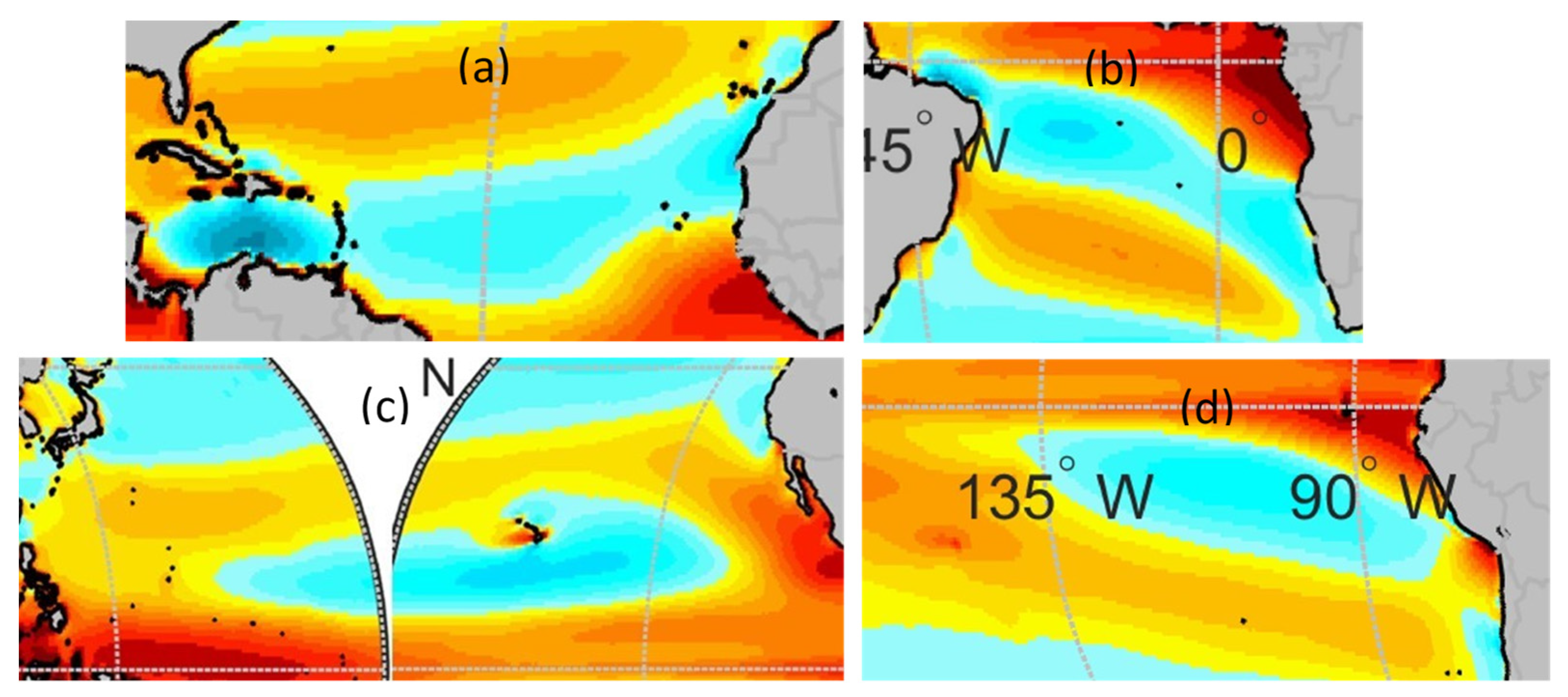
• The rest of the trade winds belts show µ₀ values between 60% and 75% and their characteristics are, see Figure 8:
• North Atlantic trade winds, Figure 8a. They initiate to the North East of Canary Islands and continue to the SW parallel to the African coast up to Cabo Blanco, turning them smoothly to the W until reaching the Lesser Antilles, where it links with the Caribbean Spot. Although there is a small strip near the coast of Mauritania with µ₀ over 70%, the rest present µ₀ values between 60% and 65%.
• South Atlantic trade winds, Figure 8b. This area of high µ₀ extend from the Cape of Good Hope in South Africa, heading towards NNW parallel to the West coast of Africa until the boundary between Namibia and Angola, were it turns to the WNW till reaching the Brazilian coast. Although µ₀ is, in general, between 60% and 70%, there are some small areas with µ₀ over 70% besides the above mentioned strip of the Northeastern Brazil coast.
• Indian Ocean trade winds, Figure 7a. This area initiates on the west coast of Australia and heads NNW until reaching the parallel 15° S, where it turns to the W until reaching San Mauricio Island (57° E) where it turns to the NW until the Northern tip of Madagascar. The mean operability in this area is in general between 60% and 70%, except the above-mentioned strip in the center of this area, where maximum values of µ₀ over 75% can be found.
• North Pacific trade winds, Figure 8c. In this area, the mean annual operability above 50% initiates at about 120° W, 15° N, heading towards the west, crossing the 180° meridian and dissipating around 155° E. To the south of Hawaii there is a large area with µ₀ above 70%, while in the rest of the area µ₀ is between 60% and 70%.
• South Pacific trade winds, Figure 8d. This trade wind belt has lower µ₀ values and extent than the abovementioned trade winds areas. The area initiates around 80° W, 18° S and heads to the WNW until 135° W, 5° S. The maximum mean annual operability in this area is between 60% and 65%.

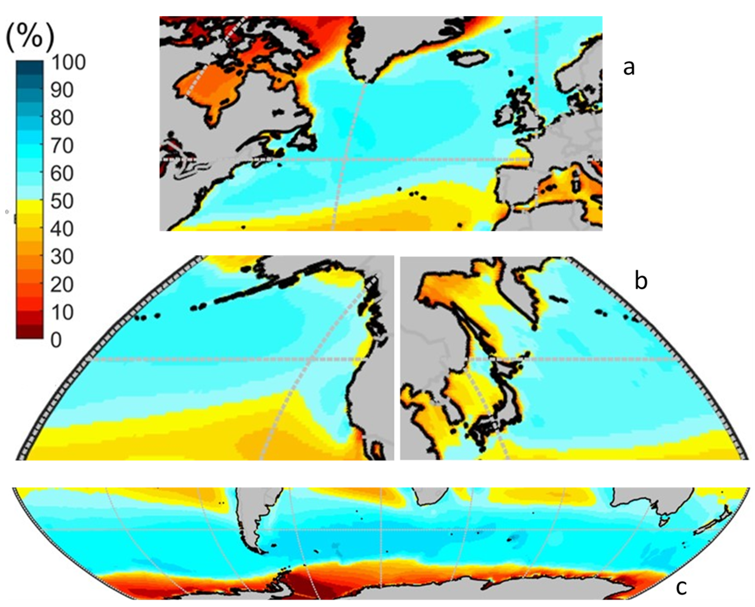
4.1.2. Annual Mean Operability in the Polar Front Belts

Polar front winds and waves arise from the mixing of the cold and warm winds blowing at surface level from the polar and subtropical high pressures, respectively. The undulating front generates area where the warm air rises over the cold, forming warm fronts, while in others the cold air entrains below the warm air forming cold fronts. In the center of the undulating fronts, a low pressure is formed and strong, very variable (in time and space) winds blow spiraling at surface level to the low center. The distribution of µ₀ in these areas is zoomed in Figure 9.

• North Atlantic polar front area, see Figure 9a. This area goes from the eastern coast of North America to the west coasts of Europe until north of Norway, including the North and Baltic Seas. To the south is limited by North Bermuda and the Azores Islands, and to the north by Greenland and Svalbard Islands. The µ₀ in this area is around 60%, with maximum values over 65% near the North America coasts and in the North Sea.
• North Pacific polar front area, Figure 9b. This large area shows similar annual mean operability levels as the Northern Atlantic with µ₀ values between 60% and 65%.
• Southern Ocean polar front area, Figure 9c. In this oceanic area, the absence of continental masses makes the polar front surround the Earth, with the only minor interruption of South America southern tip and the Antarctica Peninsula. In this large area, both strong winds and high waves limit operability and in general µ₀ is between 60% and 65% among the parallels 40° S and 55° S. From Patagonia to the Crozet Islands there is a large area with more than 70% annual mean operability.

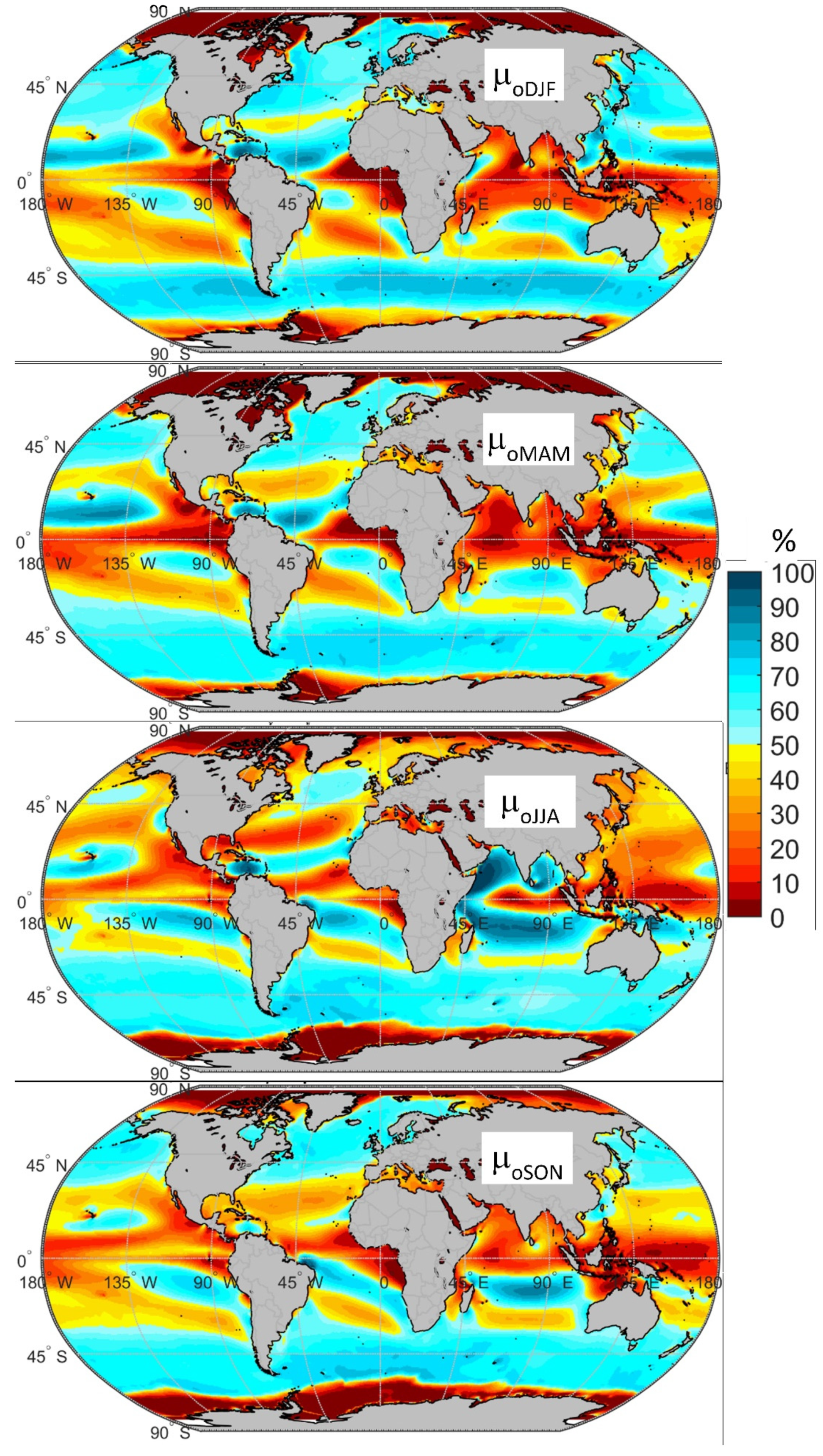
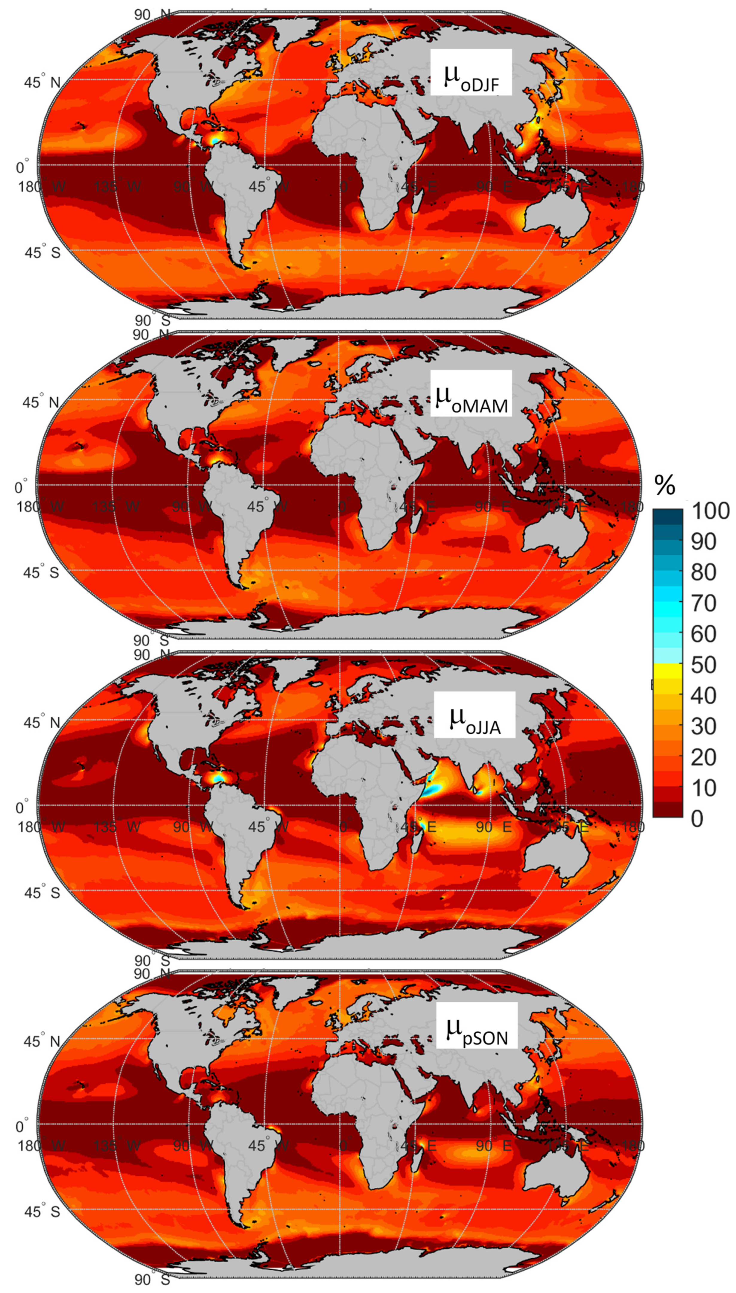
4.2. Global Distribution of the Seasonal Mean Operability

The global distribution of the seasonal mean operability, µ_0(season) is obtained by calculating in each database node the percentage of sea states in the operation range during each season: December–February (DJF), March–May (MAM), June–August (JJA), and September–November (SON). Figure 10 shows the global distribution of the seasonal operability for the four seasons.

4.2.1. North Hemisphere Distribution of the Seasonal Mean Operability.

NH Polar Belt Seasonal Mean Operability

During the NH winter (DJF), the north polar belt expands to southern latitudes and the strength of the extra-tropical storms increases. Following that pattern, the operability increases in the western sides of the North Atlantic and North Pacific Oceans, due to the wave growth limitation caused by the nearby North America, Japan Islands, and Asian continent. Due to this, the maximum mean operability values are obtained above the 30° N parallel in the western part of the Atlantic and Pacific oceans with values between 70% and 75%. In the eastern part of the Atlantic, wave height limits operability and maximum values of µ_0(DJF) are between 60–65%. The North and Baltic Seas are also partially sheltered from wave growth and maximum µ_0(DJF) range rises again to 70–75%. These high values can be found also, and for the same reasons in the Northern part of the Japan Sea.

During the NH summer (JJA) the strength of the extratropical storms decreases and the waves are no longer an operability limitation. In the North Atlantic, the maximum values of µ_0(JJA) appear in the Central and Eastern Atlantic at latitudes over 45° N (55– 60%). In the North Pacific Ocean maximum values of µ_0(JJA) are even lower (50–55%) and are located again between the parallel 45° N and the Aleutian Islands.

The spring (MAM) and autumn (SON) seasons have similar mean operability distribution, with intermediate values between the ones of winter and summer.

NH Trade Wind Belts Seasonal Operability

In the NH trade wind belts, maximum values of the mean operability occur during the winter season, i.e. (DJF). Maximum values of µ_0(DJF) can be encountered in the Central-West Atlantic (85–90%), in the Caribbean Spot (95–100%) and in very large areas of the North Pacific Ocean (80–85%). During the summer (JJA), the general trend is a decrease of µ_0(JJA), but with local increases near the coasts of Morocco and Mauritania (85–90%), and south of Hawaii (75–80%). The Caribbean Spot maintains the same very high µ_0(JJA) (95–100%) as in winter.

The mean operability during the NH spring (MAM) is very similar to the one in winter (DJF), but the autumn season (SON) shows the lowest values, with only small areas in the Eastern North Atlantic and Pacific showing mean operability over 60%, mainly near Mauritania coast and the South East of Hawaii. Only the Caribbean Spot shows mean operability levels over 70% in this season.

NH Monsoon Areas Seasonal Mean Operability

The changes in the Asian monsoon areas are remarkable. The winter monsoon (DJF) creates areas of high values of mean operability in the Southern part of the East China Sea and in the South China Sea, with maximum values between 80% and 85%, while during the summer these values fluctuate between 50% and 55%. Also noticeable are the changes due to the monsoon in the Bengal Sea, winter (DJF) 40–45%, summer (JJA) 80–85%, and in the Arabian Indian coast, winter 50–55%, summer >90%. During the summer monsoon (JJA), large areas of the Arabic Sea in the Indian Ocean reach very high (95–100%) mean operability values.

During the intermediate seasons (MAM) and (SON), the monsoon activity ceases and the mean values of operability show very low values except small spots near Somalia and Ceylon Island.

4.2.2. South Hemisphere (SH) Seasonal Mean Operability

SH Polar Belt Seasonal Mean General Operability

In the Southern Ocean, waves limit the operability, so the highest mean operability values are encountered during the corresponding summer season (DJF) with large areas having operability levels between 70% and 75%. The extension of these areas decreases in the intermediate seasons, reaching a minimum during the winter season (JJA), where these high values of mean operability are only found behind the shelter of the Southern America and Antarctic Peninsula.

SH Trade Winds Belts Seasonal Mean Operability

As in the NH, trade winds in the SH are stronger in general during the corresponding winter season (JJA), with large areas in the Indian Ocean with µ_0(JJA) values between 90% and 95%. One small spot of very high mean operability (95–100%) can be found in the north tip of Madagascar Island. In the South Atlantic, maximum values of µ_0(JJA) (80–85%) can be found in large areas between Ascension Island and the eastern tip of Brazil. An area of even higher mean operability (85–90%) can be seen in the northeastern coast of Brazil. The South Pacific trade winds area shows a large region near South America with high µ_0(JJA) values (75–80%) and another in the Eastern Pacific, near the north of Australia coast, giving maximum µ_0(JJA) levels between 90% and 95%.

The SH summer season (DJF) shows lower mean operability levels than the winter one, between 60% and 65% in the oceans, but with spots of high values in the west coast of Australia (75–80%), Atlantic Namibia coast (70–75%), and Northeastern Brazil (70–75%).

The SH spring season (SON) shows mean operability values somewhat lower than the winter season (JJA) one. The autumn season (MAM) show similar values as the summer season (JJA) but without the high operability spots of the west coast of Australia, Namibia, and Northeastern Brazil.

4.2.3. Mean Seasonal Operability Near the Coasts

Energy ships should navigate to the wind-harvesting areas and return to port to unload the produced fuel. As an alternative, they can unload at sea to another ship. In both cases, the costs of operation will be lower if operation areas for the energy ships are nearby the unloading/maintenance ports.

Table 1. (a) Ranges of maximum mean operability for the year and for the DJF, MAM, JJA and SON seasons in the polar front coastal regions. Color scale: Good (50–70%), very good (70–90%), excellent (>90%). (b) Ranges of maximum mean operability for the year and for the DJF, MAM, JJA and SON seasons in the trade winds and monsoon coastal regions. Color scale: good (50–70%), very good (70–90%), excellent (>90%).

(a)
Area	Ocean	Region	µ0	µ0	µ0	µ0	µ0
			Year (%)	DJF (%)	MAM (%)	JJA (%)	SON (%)
North Polar Front	North Atlantic	Canada	60–65	70–75	60–65	50–55	60–65
		USA	55–60	70–75	60–65	35–40	60–65
		West Norway	55–60	60–65	55–60	45–50	65–70
		West UK/Ireland	55–60	60–65	60–65	55–60	60–65
		France/Biscay Bay	45–50	60–65	50–55	35–40	50–55
		NW Spain	55–60	60–65	60–65	45–50	55–60
		Portugal	45–50	50–55	50–55	50–55	45–50
		North Sea	60–65	70–75	55–60	45–50	65–70
		Baltic Sea	55–60	70–75	45–50	40–45	60–65
	Mediterranean	Tyrrhenian	35–40	50–55	35–40	15–20	35–40
		Ionian	30–35	50–55	35–40	10–15	30–35
		Gulf of Lyon	50–55	60–65	50–55	40–45	50–55
		Aegean Sea	50–55	60–65	40–45	55–60	50–55
		Levantine	25–30	35–40	25–30	15–20	20–25
	North Pacific	Japan	55–60	75–80	55–60	40–45	60–65
		Kamchatka	50–55	65–70	50–55	40–45	60–65
		Okhotsk Sea	50–55	65–70	55–60	30–35	60–65
		Japan Sea	50–55	75–80	50–55	30–35	55–60
		Alaska	50–55	65–70	55–60	40–45	55–60
		NW USA/Canada	50–55	55–60	50–55	45–50	50–55
		California	55–60	45–50	60–65	60–65	50–55
South Polar Front	Southern Ocean	South Argentina	70–75	70–75	70–75	70–75	70–75
		Centre/S Argentina	55–60	60–65	60–65	60–65	55–60
		SE South Africa	55–60	60–65	60–65	60–65	60–65
		SW Australia	60–65	50–55	50–55	60–65	55–60
		SE Australia	60–65	60–65	60–65	60–65	60–65
		West New Zealand	60–65	55–60	60–65	60–65	60–65
		East New Zealand	60–65	55–60	60–65	60–65	60–65
		South West Chile	65–70	75–80	65–70	60–65	65–70
(b)
Area	Ocean	Region	µ0	µ0	µ0	µ0	µ0
			Year (%)	DJF (%)	MAM (%)	JJA (%)	SON (%)
North Trade Winds	Atlantic	Morocco-Senegal	65–70	65–70	80–85	85–90	60–65
		Cape Vert Islands	55–60	70–75	65–70	55–60	50–55
		Guianas coast	50–55	70–75	70–75	25–30	50–55
		Venezuela Caribbean	80–85	85–90	85–90	>90	60–65
		Caribbean Spot	85–90	>90	85–90	>90	70–75
	Pacific	South Hawaii	70–75	75–80	80–85	85–90	60–65
		Taiwan-Philippines	45–50	65–70	45–50	35–40	65–70
South Trade Winds	Atlantic	Namibia	65–70	70–75	65–70	70–75	70–75
		NE Brazil coast	75–80	75–80	60–65	>90	>90
	Indian Ocean	South Madagascar	60–65	65–70	60–65	60–65	75–80
		North Madagascar	60–65	30–35	55–60	>90	80–85
		West Australia	60–65	80–85	55–60	50–55	60–65
	Pacific	Central E Australia	50–55	50–55	50–55	50–55	55–60
		NE Australia	60–65	25–30	60–65	85–90	65–70
		Central Chilean	60–65	65–70	60–65	60–65	65–70
Asian Monsoon	Indian Ocean	Bengal Sea	40–45	40–45	50–55	80–85	35–40
		NW and SE Ceylon	55–60	50–55	40–45	>90	55–60
		Arabian Coast	45–50	50–55	35–40	>90	25–30
		Somalia Coast	65–70	80–85	35–40	>90	55–60
	E China S.	N Taiwan	60–65	80–85	55–60	50–55	65–70
	S China Sea	S Taiwan	55–60	80–85	45–50	35–40	65–70
		SE Vietnam	55–60	85–90	35–40	60–65	55–60

a shows the maximum ranges of mean operability for the year and (DJF), (MAM), (JJA) and (SON) seasons in the coastal regions of the polar front belts. Here coastal regions are considered as these offshore areas located one day or less of navigation from the coast (around 500 km). As can be seen in Table 1a, in the northern hemisphere, the operability conditions during the winter season of the Atlantic, Mediterranean, and Pacific coastal areas are in general good. The eastern coasts of USA and Canada, the North and Baltic Seas, the eastern coast of Japan, the northern part of the Japan Sea, and Southeastern Argentina show very good conditions for the energy ships operations during the corresponding winter season. Some coastal regions, as are the western coast of Norway, Scotland, and Ireland, southwest of Chile have the maximum mean operability limited by high waves and winds in winter. During the summer season, the NH operability conditions decrease clearly, while during the SH summer season (DJF) the reduction of operability is much lower or even there are better conditions in summer than in winter, as is the case of the Southwest Chilean coast that has excellent conditions in summer. The intermediate seasons, (MAM) and (SON) show mean operability ranges intermediate between the corresponding winter and summer seasons.

Table 1b show the maximum ranges of mean operability for the year and (DJF), (MAM), (JJA) and (SON) seasons, in the trade winds and monsoon coastal regions. As can be seen, in general these areas show better operability conditions than the polar front belts at least in one of the seasons.

In general, the trade winds belts show better mean operability conditions during the corresponding winter and spring seasons. The worst conditions in these areas occur during the corresponding autumn season, although in general mean operability conditions are good or very good all year round. Some areas as the Venezuela Caribbean, the Caribbean Spot, the Northeast Brazilian coast, and the south of Hawaii, show very good or excellent conditions most of the year.

The areas affected by the Asian monsoon show higher mean operability seasonal variations, with maximum mean operability values during the summer monsoon season (JJA). During this season, the Bengal Sea and Arabian Sea coasts have very good to excellent operability conditions. These conditions worsen in the other seasons, and only small areas in the NW and SE of Ceylon and Somalia remain with good conditions during the spring (MAM) and autumn (SON) seasons.

4.3. Annual Mean Duration of Operability and Non-Operability Intervals

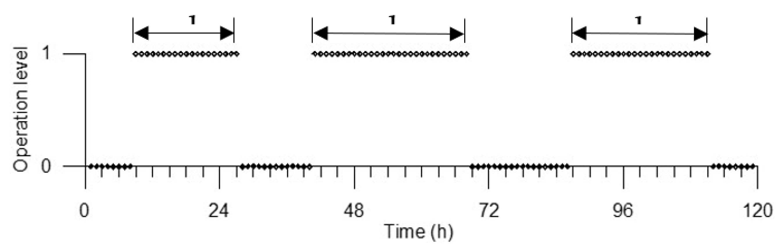
Energy ships harvest wind energy and convert it to fuel using the generated electricity and an electro-chemical installation on-board to produce hydrogen and the synthetic fuel. These chemical installations need to work at a steady pace, so some hydrogen buffer is needed to stabilize the fuel production. Additionally, the number of electrolyzers and the fuel production units depend on the duration of the non-operability intervals.

If the time series of operability in a given point is represented as a steep curve having, for example +1 for operation and 0 for no operation, the duration of operability intervals are, d1, d2, d3, …, dn, where “n” is the total number of operation intervals in the time series, see Figure 11.

For a given mesh point, the time series mean duration of operability intervals, ${\mathsf{\mu }}_{\mathrm{d}}$ is given by the Equation (4):

$${\mathsf{\mu }}_{\mathrm{d}}=\frac{1}{\mathrm{n}}{\displaystyle \sum }_{\mathrm{i}=1}^{\mathrm{n}}{\mathrm{d}}_{\mathrm{i}}$$

(4)

If the duration of the time series of general operability, S, is very long, the mean duration of non-operability intervals, µ_dno, can be obtained from Equation (4) using the Equation (5):

$${\mathsf{\mu }}_{\mathrm{dno}}=\frac{\mathrm{S}}{\mathrm{n}}{-\mathsf{\mu }}_{\mathrm{d}}$$

(5)

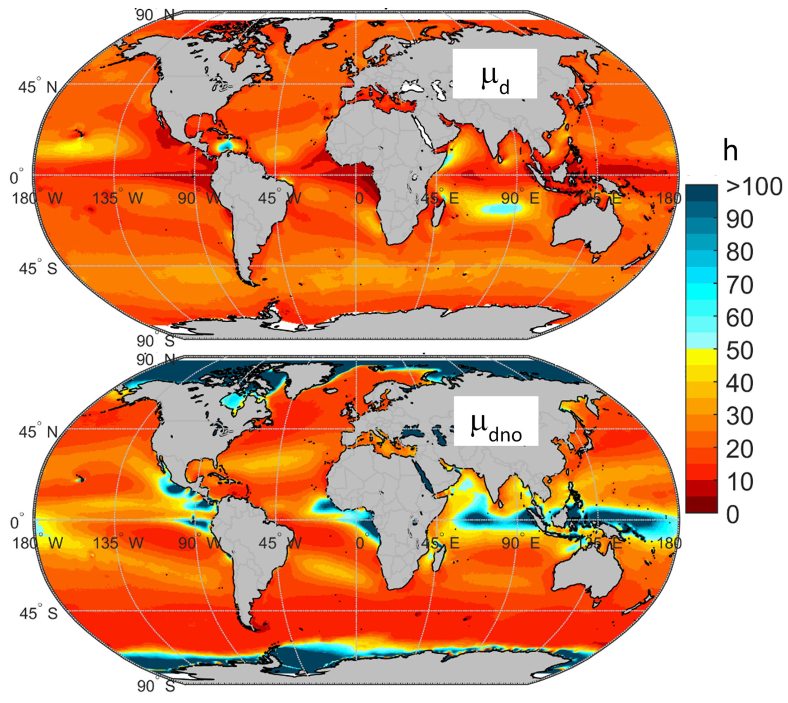
The upper part of Figure 12 shows the global distribution of the annual µ_d. As can be seen in this figure, the trade wind belts are the areas with the highest annual µ_d. In the North Atlantic trade wind belt the maximum µ_d values are in the Western side and near the Mauritania coast with mean durations ranging between 30 and 40 h. Special mention is the Caribbean Spot, with maximum µ_d values longer than 80 h. In the North Pacific trade wind belt there is a large area south of Hawaii with µ_d values between 40 and 50 h. In the southern hemisphere trade winds stands out a large area in the Indian Ocean with µd between 50 and 60 h.

Other spots of high annual µ_d are related with the Asian-Africa monsoons. These are the Indian Sea areas of the Ethiopia coast near the Horn of Africa (55–60 h), the north tip of Madagascar (55–60 h), the southeast of Ceylon Island (45–50 h), and the southeastern coast of Vietnam (40–45 h) in the South China Sea. Related to monsoon and trade winds the Taiwan Strait and the Bashi Channel between Taiwan Island and the Philippines Islands show spots having µ_d between 35 and 40 h.

The polar front belts show in general lower mean duration of operability intervals than the trade wind belts as a consequence of the higher weather variability due to the passage of the polar front storms. In these polar front areas the µd values range around 20–25 h in the NH and 25–35 h in the SH.

The global distribution of the annual mean duration of non-operability intervals, µ_dno, see the lower Figure 12, show minimum values of µ_dno in the areas of high mean general operability as are the trade winds belts and polar front belts. Minimum values of mean duration of non-operability intervals in both the polar front and the trade wind belts are between 10 and 20 h although there are spots with lower values (5–10 h) in those areas with very good mean operability values as the Caribbean Spot or the Atlantic in the southeast of Argentina.

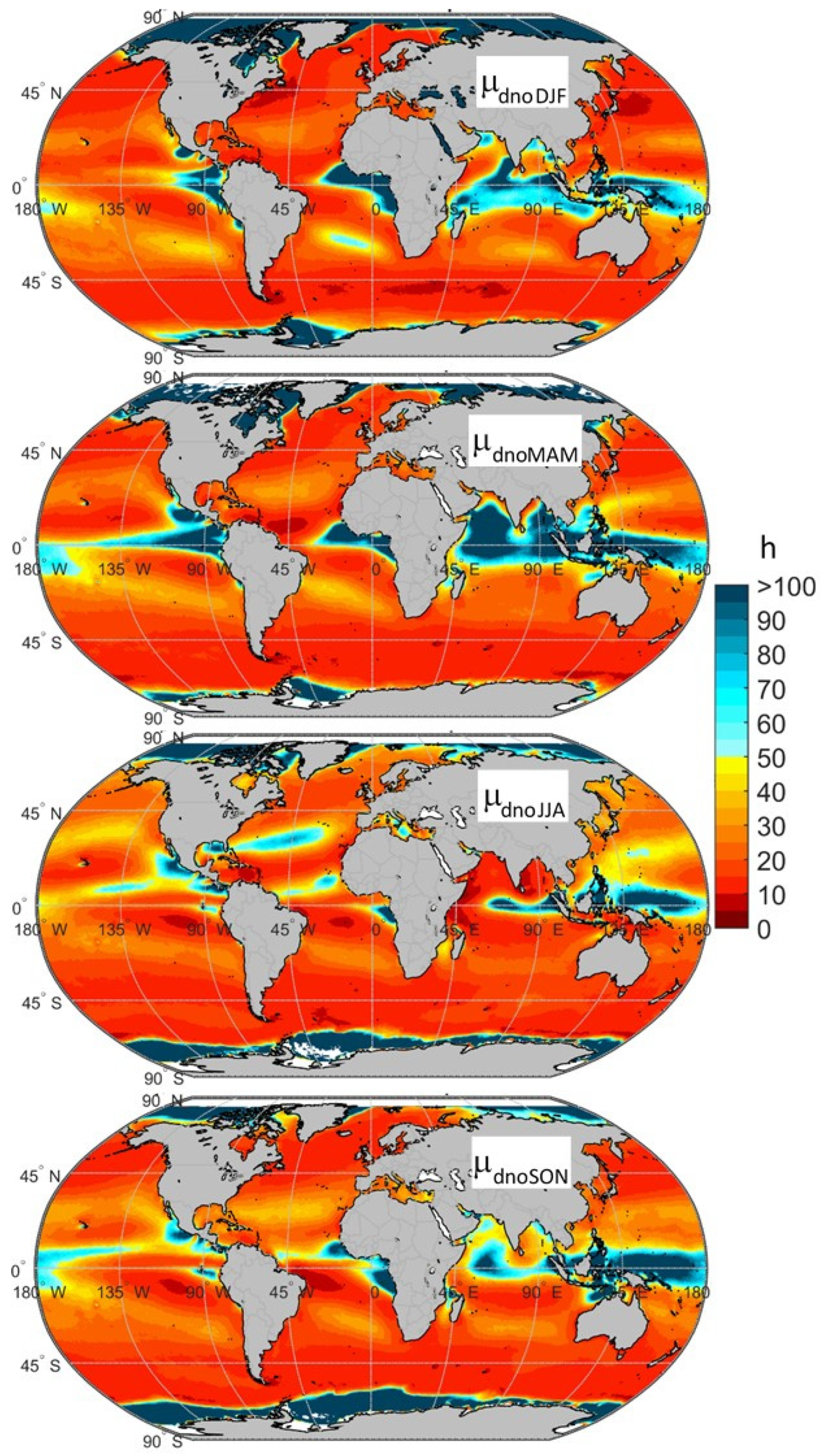
Figure 13 shows the global distribution of the seasonal mean duration of non-operability intervals. In the NH polar front belts, the lowest values (5–10 h) of µ_dno are found during the winter season (DJF) in the wave-sheltered areas near the Atlantic coasts of USA and Canada, and in the Pacific coast of the Northern Japan Islands. In the SH polar front belt, the same low values of µ_dno can be found in large patches of the Southern Ocean during the summer season (DJF).

It is noticeable the large seasonal variability in the Indian Ocean affected by the Asian monsoon as in the Bengal and Arabian seas. In the trade wind belts, the seasonal variability of µ_dno is smaller, with a general N-S displacement in latitude of the areas with minimum µ_dno durations. The largest areas of minimum µ_dno durations (5–10 h) occur during the NH spring (MAM) in the Western part of the North Atlantic trade belt and also during the SH spring (SON) in the central part of the Indian Ocean, in the Western part of the South Atlantic Ocean and in the eastern part of the South Pacific Ocean trade belts.

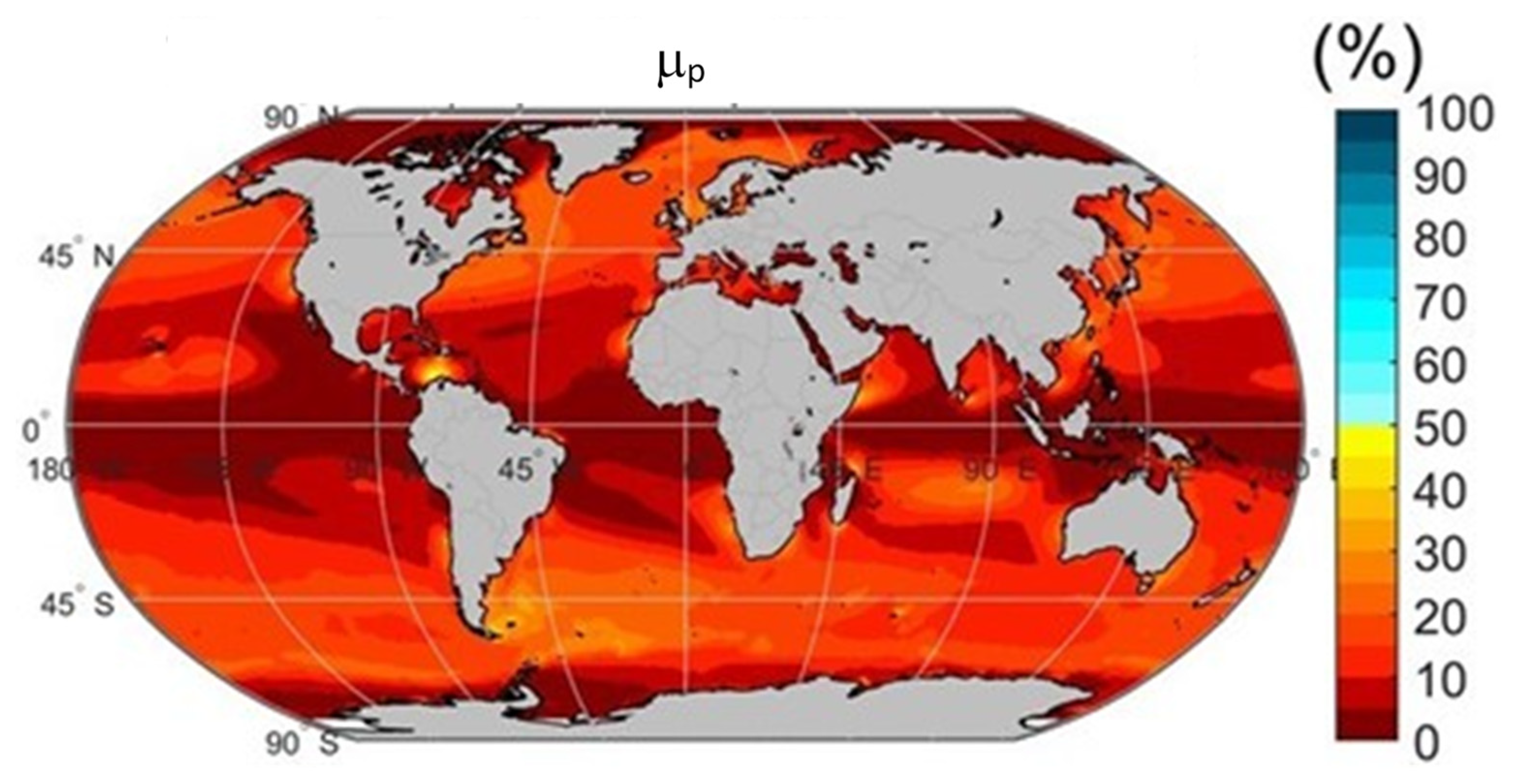
4.4. Global Distribution of the Annual Mean Optimal Operability

The global map of the annual mean optimal operability, µ_p, has been obtained calculating in each data base node the number of sea states having mean wind velocity between 10 and 15 m/s and significant wave height lower than 4 m. The seasonal mean optimal operability, µ_pseason follows the same criteria applied to the corresponding season.

Figure 14 shows the global distribution of µ_p. As the criteria for optimal operability is much more restrictive than those stablished for operability, the µ_p values are much lower than the µ₀ ones, see Figure 5. Again, the trade wind belts show the largest values of µ_p. The maximum values in each oceanic region are:

• North Atlantic trade wind belt: near the coast of Morocco and Mauritania (30–35%) and in the Caribbean Spot (45–50%).
• South Atlantic trade wind belt: Namibia coast and Northeast Brazil (30–35%)
• North Pacific trade wind belt: Southern tip of Hawaii (20–25%).
• South Pacific trade wind belt: Central Chilean coast (30–35%)
• Indian Ocean trade wind belt: a large ocean area in the center of the trade wind belt (25–30%) and northern tip of Madagascar (40–45%).
• Asian Ocean monsoon areas: South West tip of Ceylon (35–40%), Somalia coast (35–40%), SE Vietnam (30–35%), and the north of Taiwan in the East China Sea (35–40%).

In the rest of the trade wind belts, annual mean optimal operabilities are lower, with values of µ_p around 5–10% in the North and South Atlantic, 10–15% in the North Pacific, and 15–20% in the central Indian Ocean.

In the NH polar front belt, general values of µ_p are between 15% and 20%, with large areas between 20% and 25% in the Western North Atlantic, Baltic Sea, and North Sea (20–25%). Most of the Mediterranean areas show values between 10–15%. In the North Pacific polar front belt the general values are between 15% and 20%. The Pacific US coast of Oregon and California shows spots with 20–25% optimal operability.

In the SH polar front belt, the high waves limit the optimal operability with general values around 15–25%, with large areas of Argentina’s Tierra del Fuego (sheltered from the high waves coming from the west) having 30–40% mean optimal operability. The effect of wave height in the optimal operability can be seen in the eastern side of the Antarctic Islands (see, for example, the Kerguelen Islands (35–40%) or in the southeast of Australia and eastern coast of Tasmania Island (25–30%)).

4.5. Global Distribution of the Seasonal Mean Optimal Operability

Figure 15 shows the global distribution of the seasonal mean optimal operability. In general, both in the trade wind belts and polar front areas, the optimum operability is greater in the corresponding hemisphere winter. However, in the Southern Ocean polar front belt, the high waves in the winter season (JJA) reduces the optimum operability that is in this area lower than in the summer season (DJF). In the trade winds belts, stands out the high winter (JJA) optimum operability level in the Indian Ocean (35–40%).

The Asian monsoon also shows a very high seasonal variability and in the summer monsoon, optimal operability in the Indian Ocean near the Somalian coast reaches values as high as 90%, while in spring (MAM) reduces to 10–15%. Other monsoon spots with high mean optimum operability and seasonal variability are those located in the North and South Chinas Seas, reaching maximum values between 50 and 60% during the winter monsoon, while in spring (MAM) maximum values are between 10 and 15%. Here stands out the southeastern coast of Vietnam with high values of optimal operability both in winter (50–60%) and summer (40–45%).

During the winter season (DJF) in the North Atlantic maximum values of µp(DJF) of 30-35% are reached near the US east coast and in the Baltic Sea, reaching 35–40% in the North Sea, because the wave sheltering effect of the coasts. In the North Pacific, similar maximum values are reached near the Japanese Islands coasts (30–35%), for the same reasons.

The Caribbean Spot stands out from all the other spots because the optimum operability is high all year round with ranges between 65–70% in winter (DJF) and summer (JJA) and lower values (45–50%) during spring (MAM) and autumn (25–30%).

4.6. Mean Seasonal Optimum Operability Near the Coasts

The maximum seasonal mean optimum operability near the world coasts is provided in

Table 2. (a) Ranges of maximum seasonal mean optimum operability near the world coasts in the polar fronts. Color scale: Good (20–35%), very good (35–50%), excellent (> 50%). (b). Ranges of maximum seasonal mean optimum operability near the world coasts in the trade wind belts, and the Asian monsoon areas. Color scale: Good (20–35%), very good (35– 50%), excellent (> 50%).

(a)
Area	Ocean	Region	µ0	µ0	µ0	µ0	µ0
			Year (%)	DJF (%)	MAM (%)	JJA (%)	SON (%)
N Polar Front	Atlantic	Canada	20–25	30–35	25–30	10–15	25–30
		USA	20–25	30–35	25–30	5–10	20–25
		West Norway	15–20	15–20	20–25	15–20	25–30
		West UK/Ireland	10–15	10–15	15–20	15–20	20–25
		France/Biscay Bay	5–10	15–20	10–20	5–10	5–15
		NW Spain/Portugal	10–15	15–20	15–20	15–20	15–20
		North Sea	20–25	35–40	20–25	15–20	30–35
		Baltic Sea	15–20	30–35	15–20	10–15	25–30
	Mediterranean	Tyrrhenian	10–15	15–20	10–15	0–10	10–15
		Ionian	10–15	15–20	10–15	0–5	5–15
		Gulf of Lyon	15–20	20–25	15–20	10–15	15–20
		Aegean Sea	15–20	25–30	10–15	15–20	15–20
		Levantine	5–10	10–15	5–10	0–5	0–5
	Pacific	Japan	20–25	35–40	25–30	10–15	15–20
		Kamchatka	15–20	25–30	15–20	10–15	25–30
		Okhotsk Sea	15–20	25–30	15–20	5–10	25–30
		Japan Sea	20–25	30–35	20–25	10–15	25–30
		Alaska	10–15	20–25	15–20	10–15	15–20
		NW USA/Canada	10–15	15–20	10–15	15–20	10–15
		California	20–25	15–20	25–30	30–35	20–25
S Polar Front	Southern Ocean	South Argentina	35–40	35–40	35–40	35–40	35–40
		Centre/S Argentina	25–30	20–25	25–30	30–35	20–25
		SE South Africa	25–30	25–30	25–30	25–30	30–35
		SW Australia	15–20	20–25	15–20	15–20	15–20
		SE Australia	25–30	25–30	25–30	30–35	30–35
		West New Zealand	15–20	15–20	15–20	15–20	15–20
		East New Zealand	20–25	20–25	20–25	20–25	20–25
		South West Chile	15–20	20–25	15–20	10–15	10–15
(b)
Area	Ocean	Region	µ0	µ0	µ0	µ0	µ0
			Year (%)	DJF (%)	MAM (%)	JJA (%)	SON (%)
North Trade Winds	Atlantic	Morocco-Senegal	30–35	20–25	30–35	35–40	20–25
		Guianas	0–5	0–5	0–5	0–5	0–5
		Cape Vert Islands	10–15	20–25	15–20	5–10	5–10
		Venezuela Caribbean	35–40	30–35	30–35	50–55	20–25
		Caribbean Spot	45–50	65–70	45–50	65–70	25–30
	Pacific	South Hawaii	20–25	25–30	25–30	20–25	20–25
		Taiwan-Philippines	25–30	40–45	15–20	10–15	25–30
South Trade Winds	Atlantic	Namibia	30–35	35–40	25–30	25–30	30–35
		NE Brazil coast	30–35	20–25	10–15	35–40	45–50
	Indian Ocean	South Madagascar	30–35	30–35	25–30	30–35	40–45
		North Madagascar	40–45	5–10	15–20	70–75	50–55
		West Australia	20–25	40–45	15–20	10–15	20–25
	Pacific	Central E Australia	15–20	15–20	20–25	15–20	15–20
		NE Australia	20–25	10–15	25–30	45–50	15–20
		Central Chilean	30–35	35–40	25–30	30–35	40–45
Asian Monsoon	Indian Ocean	Bengal Sea	10–15	0–5	5–10	30–35	5–10
		SE and NW Ceylon	35–40	20–25	15–20	75–80	25–30
		Arabian Coast	20–25	5–10	5–10	70–75	10–15
		Somalia Coast	35–40	25–30	10–15	85–90	25–30
	E China S.	North Taiwan	35–40	50–55	20–25	20–25	40–45
	South China Sea	South Taiwan	25–30	45–50	10–15	10–15	30–35
		SE Vietnam	30–35	55–60	10–15	40–45	20–25

a,b for the year and the four seasons (DJF), (MAM), (JJA), and (SON) and for the same coastal regions as in Table 1a,b.

As can be seen in Table 2a, in the NH polar front areas, the eastern coasts of USA and Canada have good optimum operability conditions all seasons except during summer. In the western coasts of Ireland and Scotland high waves and strong winds limit optimum operability conditions except during the summer season. The best conditions are encountered in the North Sea, because the restricted fetch limits the wave growth.

As in the North Atlantic, the eastern coasts of the North Pacific show good conditions at least in winter and autumn. Very good conditions in winter occur in the Eastern Japanese coast. In the North America Pacific coasts, high waves and strong winds limit again the mean optimum operability in the coasts of the USA Northwest, Canada, and Alaska. The USA California coasts show good conditions all the year except during the winter season.

In the Mediterranean, only the Gulf of Lyon and the Aegean Sea have good optimum operability conditions during winter and fair conditions the rest of the year. The other regions have in general poor optimal operability conditions all the year. It should be taken into account that the global mesh resolution cannot detect small windy spots as the Gibraltar Strait and others.

In the Southern Ocean, the Eastern coasts of South America, Australia, and New Zealand, sheltered from the prevailing westerlies and associated waves have good or very good mean optimal operability conditions (as is the case of South Argentina (35–40%)). A special case is the SE coast of South Africa that shows good optimal operability (25–30%) conditions all year.

Table 2b shows the maximum values of the seasonal mean optimum operability near the coasts affected by the trade winds and Asian monsoon. In the Asian monsoon areas the seasonal variability of the optimum operability is very high. During the summer monsoon in the Indian Ocean, the optimum operability levels are excellent in the NW and SE tips of Ceylon, the coasts of Arabia and Somalia coasts. By contrast, during the spring, those areas have low to very low optimum operability levels (5–15%).

The winter monsoon, affect the areas of the East China Sea north and south of Taiwan and the southwest coast of Vietnam, that reach very good to excellent mean optimum operability levels. During summer, the Southwest Vietnam coast, affected by de summer monsoon, reaches very good operability levels again. A special case is the NW of the Taiwan Strait that has good optimal operability conditions in spring and summer, very good in autumn, and excellent in winter.

In the trade wind regions, the Morocco to Senegal coasts have very good optimum operability during the summer season (JJA) and good conditions the rest of the year. In this North Atlantic trade wind area, the Caribbean Spot show excellent optimum operability during winter and summer, very good during spring and good conditions during autumn. The nearby Caribbean coast of Venezuela also has excellent mean optimum operability conditions in summer and good conditions the rest of the year.

In the North Pacific trade winds there is an area of good mean optimum operability all year to the south of Hawaii. In the Western Pacific Ocean, the trade winds region between Taiwan and Philippines has very good optimal conditions during winter and good in autumn having fair conditions the other two seasons.

In the Southern Atlantic trade winds coastal areas, the Namibia coast has very good optimum operability conditions during summer (DJF) and good conditions the rest of the year. In the Western Atlantic façade, the Northeast Brazilian coast shows very good mean optimum operability conditions during the winter (JJA) and spring (SON) seasons, good conditions during summer (DJF), and poor conditions in autumn (MAM).

In the Indian Ocean trade winds areas, the southern tip of Madagascar has very good mean optimal operability conditions in spring (SON) and good conditions the rest of the year. The Northern tip of Madagascar is affected by the Asian monsoon, and has excellent μo conditions during the winter (JJA) and spring (SON) seasons, while the rest of the year the conditions are fair or poor.

In the Indian Ocean coasts of West Australia, the trade winds produce very good mean optimal operability conditions during the summer season (DJF), good conditions during the spring season (SON), and fair conditions the rest of the year.

In the Southern Pacific trade winds areas, the Central Chilean coast has very good mean optimum operability levels during the summer (DJF) and spring (SON), while during the other two seasons the conditions are good. The Northeastern Australia coasts have very good mean optimum operability conditions during the winter season (JJA) and good conditions during the spring season (MAM) while during the other two seasons the optimum operability conditions are fair.

5. Conclusions

Energy ships are an alternative to offshore wind energy farms anchored in very deep waters. Operation of energy ships depend on wind and wave intensities. After the definition of the mean wind velocity and the significant wave height operability ranges for these ships, global databases of wind and waves have been used to plot the global maps of:

• Annual and seasonal mean operability;
• Annual and seasonal mean duration of operability and non-operability intervals; and
• Annual and seasonal mean optimum operability.

From the analysis of these maps, the following conclusions can be drawn:

• There are four large areas of good annual mean operability, (more than 50%) in the World Oceans: the polar front and the trade wind belts.
• In the NH polar front belts, operability is limited by high waves on the Eastern side of the oceans during the winter season and maximum operability levels (70–75%) are located near the eastern coasts of North America, Japan Islands, and enclosed seas, such as the Japan Sea or the North Sea. During the summer season, the strength of the storms decrease and the best operability levels are found on the eastern side of the Atlantic and Pacific Oceans (50–60%).
• In the SH polar front belts, operability is limited by high waves at such a level that the best operability conditions occur during the summer season (DJF). Mean operability levels are in general in the 60–65% range. Again, as in the NH, the sheltering of the waves due to the coast, favors high annual mean operability levels (>70%) in the southeastern tip of the Atlantic Argentina coast.
• Overall, the annual mean operability in the trade wind belts is higher than that of the polar front belts, showing high to very high operability levels (75–90%) all year, except the corresponding autumn season (50–65%). Maximum annual mean general operability occurs during the corresponding winter season. Some smaller regions near the coasts such as the Caribbean Spot, the Venezuela Caribbean, the south of Hawaii and the northeastern coast of Brazil present very good annual mean operability conditions (75–90%). In the Caribbean Spot the mean operability during winter and summer seasons is excellent, nearly 100%.
• There are some ocean areas affected by the Asian monsoon that show very high seasonal variability in mean operability values. For example, in the Indian Ocean, the Bengal and Arabian Seas coastal regions show very high operability (80–90%) during the summer monsoon (JJA), while the rest of the year operability is only fair.
• In concordance with the operability levels, the duration of non-operability intervals shows minimum values in the polar front and trade wind belts with mean values between 10 and 20 h. In those areas with very high operability levels, such as the Venezuela Caribbean, the Caribbean Spot, the South of Hawaii and the northeast of Brazil the mean duration of non-operability intervals reduces to 5–10 h.
• The values of the mean optimum operability are much lower than those of the mean operability due to the restrictive ranges of wind and waves imposed by the optimum conditions.
• The mean optimum operability in the NH polar front coastal areas shows good values during the winter (DJF) and autumn seasons (SON) on the western side of the oceans, where the continents or islands reduce the fetch of the prevailing westerlies.
• In the SH the good mean optimum operability conditions are more permanent due to the year-round stronger wind conditions in areas sheltered from waves by the land as the South East of Argentina (35–40%), Southeast Africa, Southeast Australia, and New Zealand.
• Very good values of maximum annual mean optimum operability (35–50%) occur in the areas of good to very good maximum values of mean operability: Venezuela Caribbean, Caribbean Spot, North Madagascar, SE and NW of Ceylon, the Somalia coast, and North Taiwan.
• The seasonal variability of the mean optimum operability is very high in those areas affected by the Asian monsoon in the Indian Ocean. In these areas maximum values of the mean optimum operability occur during the summer season (JJA).
• The Venezuela Caribbean, the Caribbean Spot, and the north of Taiwan have good to excellent maximum values of mean optimum operability during all seasons. Good to very good mean optimum conditions can be found year-round near the coasts of Morocco-Senegal, Namibia, and Central Chile.

These results should be taken as a first approximation to the analysis of energy ship operability. Once the areas for optimal operation are identified, downscaled models of wind and waves should be used to improve the resolution in those small areas near coasts or islands affected by the low spatial resolution of global climate models.