Article

The Influence of Wind-Induced Waves on ENSO Simulations

1
College of Oceanography, Hohai University, Nanjing 210024, China
2
Key Laboratory of Marine Hazards Forecasting, Ministry of Natural Resources, Hohai University, Nanjing 210024, China
3
State Key Laboratory of Satellite Ocean Environment Dynamics, Second Institute of Oceanography, Ministry of Natural Resources, Hangzhou 310012, China
4
Southern Marine Science and Engineering Guangdong Laboratory (Zhuhai), Zhuhai 519080, China
5
Environmental Science and Engineering, University of North British Columbia, Prince George, BC V2N 4Z9, Canada
6
Key Laboratory of Marine Science and Numerical Modeling, First Institute of Oceanography, Ministry of Natural Resources, Qingdao 266061, China
7
Laboratory for Regional Oceanography and Numerical Modeling, Pilot National Laboratory for Marine Science and Technology, Qingdao 266237, China
8
Shandong Key Laboratory of Marine Science and Numerical Modeling, Qingdao 266061, China
*
Author to whom correspondence should be addressed.
J. Mar. Sci. Eng. 2021, 9(5), 457; https://doi.org/10.3390/jmse9050457
Submission received: 24 February 2021 / Revised: 6 April 2021 / Accepted: 14 April 2021 / Published: 23 April 2021
(This article belongs to the Section Physical Oceanography)

Abstract

:
We evaluated the influence of wind-induced waves on El Niño-Southern Oscillation (ENSO) simulations based on the First Institute of Oceanography-Earth System Model version 2 (FIO-ESM 2.0), a global coupled general circulation model (GCM) with a wave component. Two sets of experiments, the GCM, with and without a wave model, respectively, were conducted in parallel. The simulated sea surface temperature (SST) was cooled by introducing the wave model via the enhancement of the vertical mixing in the ocean upper layer. The strength of ENSO was intensified and better simulated with the inclusion of wave-induced mixing, particularly the La Niña amplitude. Furthermore, the simulated amplitude and spatial pattern of El Niño events were slightly altered with the wave model. Heat budget analyses revealed the intensification of La Niña events to be generally attributed to wave-induced vertical advection, followed by the zonal and meridional advection terms.

1. Introduction

Climate models have become a powerful tool in simulating and predicting climate anomalies and variabilities across wide temporal and spatial scales. Climate models can be generally divided into four types: atmospheric general circulation, ocean general circulation, land surface, and sea ice models. Great progress has been made over the past few decades in developing advanced coupled models, including increased resolutions and more accurate parameterization schemes. However, current climate models still face large systematic biases, typically attributed to the absence or misrepresentation of important physical processes, for example, the surface waves. Hasselmann [1] revealed the importance of surface gravity waves in numerical models; yet, previous climate models rarely consider waves, as their spatial and temporal scales are too small to be resolved in models. However, wave motion plays a key role in the physical process of the upper ocean [2,3,4,5,6,7,8,9]. For example, the spray, turbulence, and bubbles introduced by the breaking wave can influence the air–sea fluxes [3]. Sea temperature in the upper ocean is significantly affected by the vertical mixing introduced by the surface waves [10,11]. Yu et al. [12] found that the simulation of sea level pressure could be clearly improved by accounting for the effect of surface waves. Furthermore, Qiao and Huang [13] revealed that the inclusion of the nonbreaking wave-induced vertical mixing (Bv) can aid in the reduction of distribution and seasonal cycle biases of the ocean temperature. Previous work has demonstrated that considering the effects of the surface wave-induced mixing in the Community Climate System Model Version3 (CCSM3) can effectively improve the simulation of tropical basin wide sea surface temperature (SST) values [11].
The influence of waves must thus be considered in order to improve climate model performances. The First Institute of Oceanography-Earth System Model version 1.0 initially incorporated an ocean surface wave model with the global coupled Community Earth System Model (CESM) version 1 (FIO-ESM 1.0) [7]. Zhao et al. [14] compared the prediction skill of the North Pacific variability (NPV) index between FIO-ESM 1.0 and Climate Forecast System, Version 2 (CFSv2), finding that the skill of FIO-ESM 1.0 is higher by 11.6% (23.6%) when ENSO and NPV are in (out of) phase at initial conditions. Chen et al. [15] revealed that the introduction of Bv to FIO-ESM 1.0 simulated a more stable stratification, thus reducing the mixed layer depth and heat content biases. Shu et al. [16] employed FIO-ESM 1.0 to simulate the Arctic Ocean ice, indicating the ability of the model to simulate the seasonal variation of sea ice coverage and to predict the sea ice fluctuations across different conditions.
In order to improve FIO-ESM 1.0, the First Institute of Oceanography developed FIO-ESM 2.0, based on its predecessor. FIO-ESM 2.0 includes new physical processes and more detailed grids. Bao et al. [17] used the SST from the Hadley Centre Sea Ice and Sea Surface Temperature (HadISST) data [18], precipitation from the Global Precipitation Climatology Project (GPCP) data [19], and surface air temperature from (the Met Office Hadley Centre/Climate Research Unit version 4) HadCRUT4 data [20] to compare the performance of FIO-ESM 2.0 against FIO-ESM 1.0, concluding that FIO-ESM 2.0 can better represent the asymmetric precipitation around the equator, and have better simulations of surface air temperature and SST.
In the current paper, we employed FIO-ESM 2.0 to evaluate the simulation ability of ENSO and investigate the impacts of waves, which has previously been under-reported. ENSO plays a dominant role in the atmosphere–ocean interaction within the tropical Pacific, strongly affecting global climate and human activities [21,22,23,24,25,26,27,28,29]. It is characterized by the anomalous warming in the equatorial eastern tropical Pacific every 2–7 years, typically peaking at the winter season (called phase locking) [30]. In recent studies, a new type of El Niño event was discovered, called Warm pool (WP) El Niño events. Different from the conventional Cold Tongue (CT) El Niño with warming in the eastern tropical Pacific, the WP El Niño events occur with the warming near the central tropical Pacific [24,31,32,33,34]. Often, the El Niño event is defined when Nino3.4 index (SSTA averaged over 5° S–5° N, 170° W–150° W) during the boreal winter (December–January–February, DJF) is larger than its corresponding one standard deviation, whereas the Nino3 index (SSTA averaged over 5° S–5° N, 150° W–90° W) and the Nino4 index (SSTA averaged over 5° S–5° N, 160° E–150° W) are used to define WP and CT El Niño events, respectively (e.g., Yeh et al. [35]). For an El Nino event, when its Nino3 (Nino4) index is larger than Nino4 (Nino3) index, the El Niño event is defined as CT (WP) El Niño.
ENSO simulation and prediction have been an intensive research filed of the tropical air–sea interaction. Many efforts have been made to accurately simulate the ENSO features, from its period, phase locking, to irregularity, etc. Various climate models with different complexities have been developed and used towards this goal, as well documented in Coupled Models Intercomparison Project (CMIP) from CMIP3 to CMIP6 [26,27,29,30,36]. For example, Ham et al. [36] evaluated the simulation of two types of El Niño in CMIP3 models and found that most of models tended to simulate a single type of El Niño. The possible reason may be the unrealistic representation of annual-mean SST in these models. As another example, Zhang and Sun [29] concluded that the models in CMIP5 remained the problems of simulating too weak ENSO asymmetry, which is possibly due to the weak model SSTA and the wrong position of the anomaly centers. Moreover, Bellenger et al. [30] compared the simulation of ENSO from CMIP3 to CMIP5 and found that ENSO life cycle in CMIP5 is modestly improved, including the large SSTA location and seasonal phase locking.
While these ENSO models represent a full spectrum of coupled models including various physical processes and resolutions, they almost lack a wind-induced wave component in coupling systems. Chen et al. [37] employed FIO-ESM 1.0 to examine the ENSO simulation biases and found several common limitations, such as an eastward tendency of the location of El Niño, a regular period, excessive strength, and the spurious eastward propagation of El Niño events. Despite a detailed analysis on El Niño events, Chen et al. failed to discuss the La Niña simulations in detail and did not evaluate the influences of the wave model on ENSO simulations. In the current paper, we apply FIO-ESM 2.0 to further expand the investigation on the effects of waves on ENSO simulations. An emphasis is placed on ENSO properties including period, phase-locking feature, and diversity, as well as the influences of the ENSO phases.
The remainder of this paper is arranged as follows. Section 2 details the FIO-ESM 2.0 configuration and the data used in this work. Section 3 analyzes the ENSO feature simulation and the corresponding wave model influences, and discusses the potential physical processes underlying these influences on the ENSO simulations. Section 4 concludes the paper.

2. Model and Method

2.1. Model

FIO-ESM 2.0 was developed by the First Institute of Oceanography, Ministry of Natural Resources of China and includes five models: the Community Atmosphere Model version 5, with a finite-volume dynamical core (CAM5) [38]; the Community Land Model version 4.0 (CLM4.0) [39]; the Parallel Ocean Program version 2 (POP2) [40]; the Los Alamos Sea Ice Model version 4 (CICE4) [41]; and the Marine Science and Numerical Modeling (MASUM) [42]. All five models are coupled by coupler 7. CAM5 has a horizontal resolution of 0.9° × 1.25° (latitude x longitude), with 30 vertical layers. POP2 grids have a 1.1° × 0.27–0.54° resolution (longitude × latitude) and 61 vertical layers. CICE4 and MASUM have the same resolution as POP2, while the horizontal resolution of CLM4.0 is equal to that of CAM5.
The wave model, called MASNUM in FIO-ESM 2.0, introduces four distinct physical processes, including nonbreaking surface wave-induced mixing (Bv), stokes drift on air-sea fluxes, sea spray on air-sea heat fluxes, and SST diurnal cycle parameterization [17]. The Bv can be calculated as follows:
Bv = α k E k exp { 2 k z } d k z ( k ω 2 E k exp { 2 k z } d k ) 1 2 ,
where α is a constant coefficient usually set to 1.0; E k represents the wave number spectrum; ω is the wave angular frequency; k   is the wave number; and z is the vertical coordinate (upward being positive) with z = 0 at the ocean surface. Details of the remaining physical processes can be found in Bao et al.’s report [17].

2.2. Method and Data

In order to examine the influences of the waves on ENSO simulation, we conducted two experiments, namely, the wave run based on FIO-ESM 2.0 with the wave model (denoted as wave run hereafter) and the no-wave run based on FIO-ESM 2.0 without the wave model (denoted as no-wave run hereafter). A 150-year run is carried out under present-day forcing for each experiment and only the potential temperature and zonal wind stress of the last 50 years are analyzed. For comparison, we used the observed temperature and zonal wind stress during the period from 1961 to 2010. Monthly SST was taken from the Hadley Centre Sea Ice and Sea Surface Temperature dataset (HadISST) [18], while the monthly mean potential temperature and zonal wind stress were obtained from Simple Ocean Data Assimilation (SODA, version 2) [43].

3. Influences on ENSO

Prior to analyzing the simulation of ENSO events, we simulated the climate mean states from the two sets of experiments, which are able to capture the basic spatial distribution of SST (Figure 1). However, the amplitude of SST is overestimated in most areas (Figure 1e,f), including tropical, subtropical, extra tropical regions, and even some middle latitudes. The simulated SST of the wave run is observed to be cooler than that in the no-wave run (Figure 1d). The student t test is a common method to estimate the robustness of model results [44]; we used the method to make a significance test (overlaying points in Figures 1, 7, and 8). We also noticed that the significant differences mainly distribute on the southern ocean and the western Pacific. This suggests a reduction in the model warmer bias when the wave model is implemented in FIO-ESM 2.0, although the difference between the two experiments is minimal.
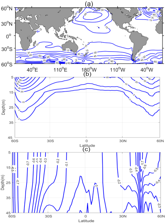
Previous studies have demonstrated that Bv introduced a great impact on the model simulation, for example, suppressing the overly westward extension of the simulated equatorial cold tongue [45] and improving the simulation of the mixed layer depth [15]. In Figure 2, the averaged Bv across the 50-year time-period is used to determine the impact of Bv on SST. Bv exhibits the same spatial pattern as Figure 1d, with large (small) values observed in high (low) latitudes, suggesting its dominant role in controlling the SST differences between the two experiments.
Figure 2b depicts the vertical distribution of the multiyear and longitudinal averaged Bv, while Figure 2c is the same, but for the difference of sea temperature between the two experiments. Figure 2b,c are similar, for example, the maximum values occur close to the global sea surface, decreasing rapidly with depth and increasing with latitude. This further confirms the influence of waves on the sea temperature simulations.

3.1. Influences on ENSO Properties

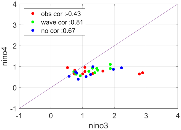
Ham et al. [36] revealed negative weak correlations between Nino3 and Nino4 indices during the El Niño years, implying the separability of WP and CT El Niño. However, the majority of climate models can only simulate one type of El Niño based on these criteria [26,36]. To explore the ability of FIO-ESM 2.0 to describe the two El Niño types, we calculated the correlation between the Nino3 and Nino4 indices during the boreal winter for the two experiments and observational data (Figure 3). The observed value is determined as −0.43, indicating that WP El Niño is independent of CT El Niño to some extent. However, the two experiments differ from the observation (Figure 3). In particular, the Nino3 and Nino4 indices are highly correlated (0.81 and 0.67 for the wave and no-wave runs, respectively). This indicates the inability of FIO-ESM 2.0 to explain the two El Niño types, irrespective of the inclusion of the wave model. Thus, the WP and CT El Niño events remain unseparated in the following discussions.
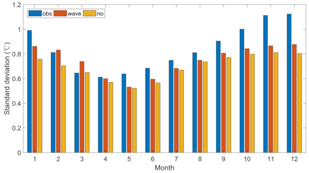
Following previous work [30], we employed the standard deviation of the Nino 3 index to examine the phase locking in the two experiments. Figure 4 presents the standard deviation of each calendar month from the observational data and the two experiments. The maximum and minimum standard deviations of the observations are observed in December and April, respectively. Both experiments are able to reproduce the phase locking feature, with the largest standard deviations occurring in boreal winter. The standard deviation can be an effective indicator of the ENSO event strength [26]. The observed ENSO event strength is underestimated in the two experiments (Figure 4). However, the simulated ENSO amplitude is stronger and closer to the observation in the wave run compared to the no-wave run.
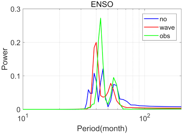
ENSO has an irregular broadband period ranging from 2 to 7 years [30]. Figure 5 depicts the power spectrum of the Nino3 index determined from the observational data and the two experiments. The observational data exhibits two major periods of approximately 3.5 and 4.7 years, with the first of a larger variance. However, the no-wave run power spectra of the Nino 3 index demonstrate multiple peaks, but a lower variance. This suggests the lack of a principal period. The inclusion of the wave model results in two obvious periods with a much larger variance centered at 3.3 years, indicating the stronger performance of the wave run in simulating the ENSO period.

3.2. Influences on El Niño and La Niña

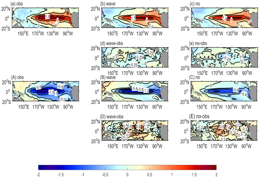
We implemented composite analysis to explore the impacts of the wave model on the ENSO phases. El Niño and La Niña events were selected when Nino 3.4 index was larger or smaller than its one standard deviation during the boreal winter, respectively. Figure 6 presents the spatial distribution of the SST anomalies during the boreal winter of the El Niño and La Niña events. The amplitudes of the El Niño events are underestimated by approximately 0.2 °C in both experiments. The influence on the distribution and amplitude of the warm phase is limited, irrespective of the inclusion of the wave model.
The observed results demonstrate the cooling anomalies of the La Niña events to be concentrated in the Nino3.4 region, with an averaged amplitude of −1.6 °C close to the equator (2° S–2° N, 170° W–120° W). However, in the no-wave run, the simulated SST anomalies are restricted around the equator and the intensity is underestimated compared to the observational data, with an averaged value of −1 °C. The inclusion of the wave model enhances the La Niña, with an SSTA of −1.3 °C close to the equatorial region. This is in stronger agreement with the observation compared with the no wave run and suggests that the inclusion of the wave model to FIO-ESM 2.0 can relieve the weak bias of La Niña, particularly near the equator.
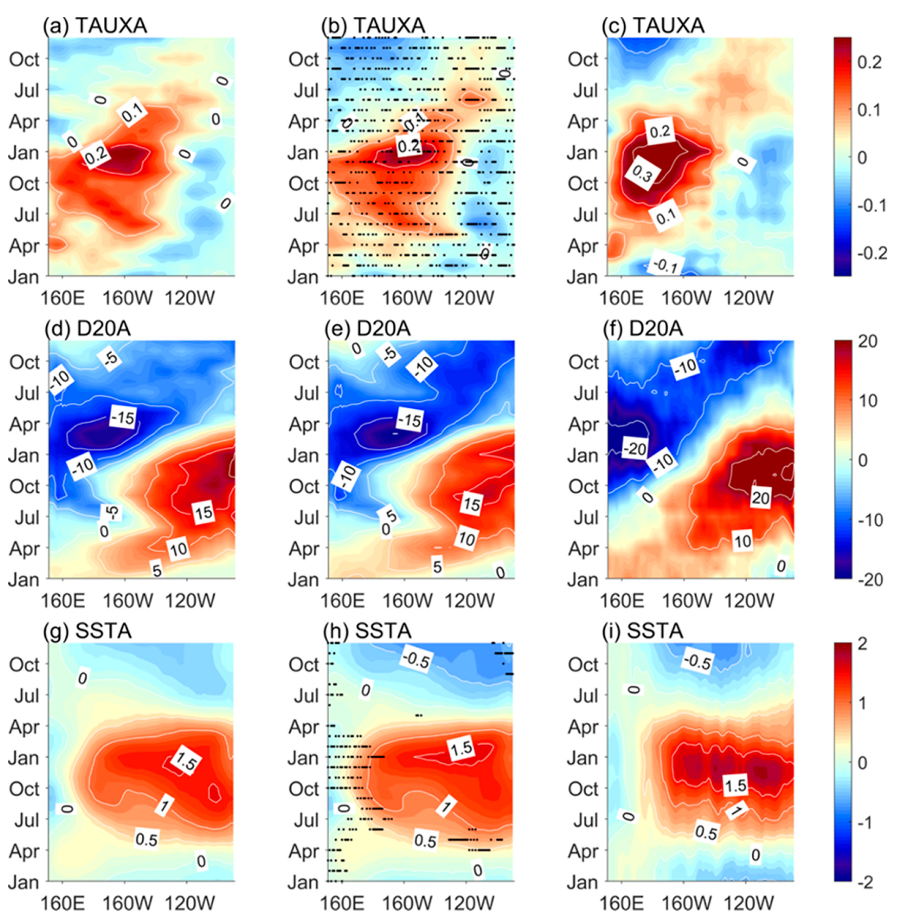
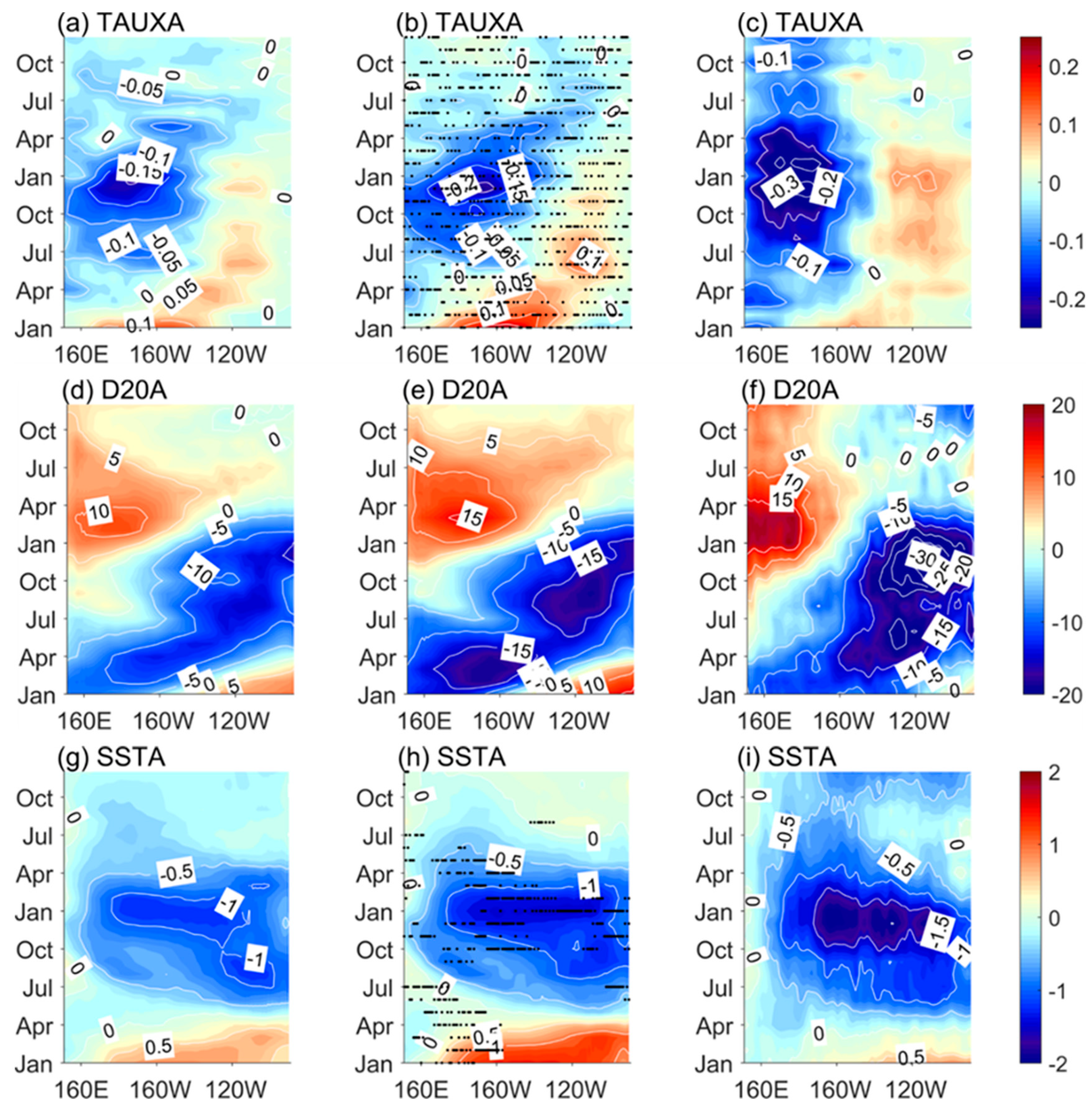
In order to further depict the influences of the wave model on different ENSO phases, we derived the evolution of SSTA, D20 anomalies, and zonal wind stress anomalies averaged from 2° S to 2° N are derived during El Niño and La Niña cycles (Figure 7 and Figure 8, respectively). In the observation, westerly wind stress anomalies prevail over the western and central Pacific during the development and mature phase of El Niño. Accompanied by the wind anomalies, the thermocline deepens over the eastern Pacific and lifts over the western Pacific. As a result, the warming SSTA over the equatorial eastern Pacific are enhanced and peak during the boreal winter. In the no-wave run, the westerly wind stress and thermocline depth anomalies are both weakly simulated, which consequently weakens the simulated strength of El Niño to below that of the observation. The statistically significant test shows that the wind-induced waves have significant impact on both zonal wind stress anomalies and SSTA over considerable areas as highlighted by dots. However, the differences between wave run and no-wave run are not significant for thermocline anomalies, probably because the impact of wave are manifested on upper ocean. The introduction of the wave model slightly changes the evolution of the wind stress, thermocline depth, and SST anomalies. This indicates the minimal effect of the wave model on the El Niño simulation, which is consistent with the composite analysis in Figure 6. Figure 8 depicts the wind stress anomaly simulations in the no-wave run of the La Niña cycles. Similar to the El Niño events, the easterly wind stress anomalies are significantly underestimated, resulting in weaker thermocline depth anomalies and SSTA. In the wave run, the simulation of the easterly wind stress anomalies is enhanced, accompanied with much stronger and closer-to-observation thermocline depth anomalies. This suggests the obvious reduction in the bias of the thermocline depth anomalies for the wave run. As expected, the SSTA are clearly strengthened during the La Niña peak phase. Similar to El Niño events, the significant differences between the two runs also only occur for wind anomalies and SSTA.
Figure 7 and Figure 8 demonstrate that the El Niño and La Niña simulations in the no-wave run suffer from the biases of weak surface wind stress anomalies, thermocline depth anomalies and SSTA with respect to the observational data. The wave model has little influence on the simulation of El Niño, and significantly improves the La Niña simulations. This improvement is generally observed in the strength of cold events rather than the cold location. Such an asymmetric impact of waves on El Niño and La Niña events may be attributed to the interaction between ocean climatological states and waves. During the La Niña events, the thermocline is shoaling in the eastern Pacific. The wave-induced mixing has a great effect on the evolution of SSTA due to the shallow mixed layer. However, during El Niño events, SSTA are not affected by the waves because of the deeper mixed layer and thermocline depth in the eastern Pacific ocean.

3.3. Heat Budget Analysis

In order to further explore the effects of the wave model on the simulation of La Niña events, we conducted a heat budget analysis of the mixed layer (from the surface to 50 m depth) during the cold events. Following Kug [24], we derived the temperature equation as follows:
t T = u x T - u - x T u x T zonal   advection v y T - v - y T v y T meridional   advection w z T - w - z T w z T vertical   advection + R
where u, v, w, and T represent the zonal, meridional, vertical current, and the temperature averaged from 5° S to 5° N in the mixed layer, respectively; the overbars and primes indicate monthly climatology and anomalies, respectively; and R represents the residual term.
Figure 9 depicts the temperature anomaly tendency ( t T ), the zonal advection ( u x T - u - x T u x T ), meridional advection ( v y T - v - y T v y T ), and vertical advection ( w z T - w - z T w z T ) terms, respectively, averaged over 9 months prior to the maximum cooling that spans the entire period of an event from the developing to mature phase. All three advections in the no-wave run are responsible for the development of the La Niña events. The vertical advection exerts the greatest contribution, followed by the meridional and zonal advections. The introduction of the wave model results in an obvious increase in the temperature anomaly tendency by 0.05 / month , indicating the enhancement of the La Niña event strength. This is consistent with the results discussed in Section 3. The zonal, meridional, and vertical advection terms contribute to the increased temperature anomaly tendency by approximately 0.02, 0.04, and 0.02 ( / month ), respectively. Despite the maximal increase in the meridional advection, the vertical advection is still the dominant contributor to the development of La Niña. The increased vertical advection may be attributed to its inherent association with nonbreaking wave-induced mixing. In short, the three advection terms are all intensified by the introducing of the wave model during the La Niña development, resulting in the enhanced strength of La Niña events.

4. Conclusions

ENSO is an important climate phenomenon that has great impacts on the global climate and weather. Since the first coupled ENSO model was developed, various types of coupled models have been designed and used for ENSO simulation and prediction, including simple models, intermediate coupled models, hybrid coupled models to fully coupled general circulation models (GCMs). With these efforts, significant progress of ENSO simulation has been made over the past four decades. However, there are still great challenges in simulating some features of ENSO. For example, many CGCMs cannot well simulate ENSO diversity, whereas warming anomalies are also often squeezed near the equator [26,27,30,36].
To improve ENSO simulation, we explored the role of wind-induced waves in ENSO features in this paper, which are absent in most of current climate models. For this purpose, we conducted two sets of experiments using FIO-ESM 2.0 with and without a wave model to determine the impacts of wind-induced waves on ENSO. In particular, we compared the two experiments in terms of the strength, period, phase locking, and phases of ENSO. The key findings and conclusions are summarized in the following:
(1)
In both experiments, the simulation of SST suffers from a basin-wide warm bias. The inclusion of the wave model to FIO-ESM 2.0 reduces the warm bias to some extent, particularly in the extratropical region. Differences in the SST between the two experiments have similar spatial distribution to the Bv, with large values in high latitudes and low values in low latitudes. Further analysis demonstrates that the nonbreaking wave-induced vertical mixing influences the SST simulations.
(2)
FIO-ESM 2.0 is unable to effectively characterize the two types of El Niño events (i.e., WP El Niño and CT El Niño). Moreover, the impact of waves on ENSO diversity is limited.
(3)
The two experiments are able to reproduce the phase locking feature, yet they tend to underestimate the strength of ENSO events. This bias is slightly reduced when the wave model is introduced into FIO-ESM 2.0. The wave model can also improve the ENSO period simulations.
(4)
The wave model has little influence on the simulation of the El Niño strength. However, the bias in the simulation of the La Niña amplitude is significantly reduced. Without the wave model, the cooling anomalies are clearly underestimated and restricted around the equator in FIO-ESM 2.0. The inclusion of the wave model increases the maximum amplitude of the cooling anomalies, resulting in values much closer to the observation. In short, the wave model exerts asymmetric influences on El Niño and La Niña events. This can be attributed to the different ocean states. During El Niño events, the thermocline is deep in the east, and thus the wave-induced mixing has little impact on SST anomalies. However, during La Niña events, the thermocline is shallow in the east, which facilitates the upwelling of the cold water to the surface by wave-induced mixing, strengthening the amplitude of La Niña.
(5)
Heat budget analysis of the mixed layer revealed that when the wave model is introduced into FIO-ESM 2.0, the vertical, zonal, and meridional advection terms are strengthened. This consequently amplifies the intensity of La Niña and improves simulation accuracy.
The wave model consists of four processes: the Bv; stokes drifts on air–sea fluxes; sea spray on air–sea heat fluxes; and SST diurnal cycle parameterization [17]. In this paper, the individual impacts of the four processes are not separated; rather, they are all turned off in the no-wave run and turned on in the wave run. Based on previous studies [37,44] and the high similarity of the SST differences between the two experiments and Bv, we suggest that the impact of waves on ENSO originates from the contribution of Bv. The effects of the three waved-related processes (the stokes drift on air–sea fluxes, sea spray on air-sea heat fluxes, and SST diurnal cycle parameterization) are likely to be minimal. The confirmation of this is reserved for future work.

Author Contributions

Conceptualization, Y.H., X.T., and Y.T.; methodology, Y.H., X.T., and Y.T.; software, Y.H., Z.S., and Y.B.; writing—original draft preparation, Y.H.; writing—review and editing, X.T. and Y.T. All authors have read and agreed to the published version of the manuscript.

Funding

This study was supported by grants from the National Key R&D Program of China (2017YFA0604202), and the National Natural Science Foundation of China (41690124, 41690120, 41806038, 41806032).

Institutional Review Board Statement

Not applicable.

Informed Consent Statement

Not applicable.

Data Availability Statement

Not applicable.

Conflicts of Interest

The authors declare no conflict of interest.

References

  1. Hasselmann, K. Ocean circulation and climate change. Tellus A 1991, 43, 82–103. [Google Scholar] [CrossRef] [Green Version]
  2. Babanin, A.V.; Ganopolski, A.; Phillips, W.R. Wave-induced upper-ocean mixing in a climate model of intermediate com-plexity. Ocean Model. 2009, 29, 189–197. [Google Scholar] [CrossRef]
  3. Cavaleri, L.; Foxkemper, B.; Hemer, M.A. Wind Waves in the Coupled Climate System. Bull. Am. Meteorol. Soc. 2012, 93, 1651–1661. [Google Scholar] [CrossRef]
  4. Craig, P.D.; Banner, M.L. Modeling Wave-Enhanced Turbulence in the Ocean Surface Layer. J. Phys. Oceanogr. 1994, 24, 2546–2559. [Google Scholar] [CrossRef] [Green Version]
  5. Huang, C.J.; Qiao, F.; Dai, D. Evaluating CMIP5 simulations of mixed layer depth during summer. J. Geophys. Res. Ocean. 2014, 119, 2568–2582. [Google Scholar] [CrossRef]
  6. Mellor, G.L.; Blumberg, A.F. Wave Breaking and Ocean Surface Layer Thermal Response. J. Phys. Oceanogr. 2004, 34, 693–698. [Google Scholar] [CrossRef]
  7. Qiao, F.; Song, Z.; Bao, Y.; Song, Y.; Shu, Q.; Huang, C.; Zhao, W. Development and evaluation of an Earth System Model with surface gravity waves. J. Geophys. Res. Ocean. 2013, 118, 4514–4524. [Google Scholar] [CrossRef]
  8. Wunsch, C.; Ferrari, R. Vertical mixing, energy, and the general circulation of the oceans. Annu. Rev. Fluid Mech. 2004, 36, 281–314. [Google Scholar] [CrossRef] [Green Version]
  9. Zhao, B.; Qiao, F.; Wang, G. The effects of the non-breaking surface wave-induced vertical mixing on the forecast of tropical cyclone tracks. Chin. Sci. Bull. 2014, 59, 3075–3084. [Google Scholar] [CrossRef]
  10. Chuanjiang, H.; Fangli, Q.; Zhenya, S. The effect of the wave-induced mixing on the upper ocean temperature in a climate model. Acta Oceanol. Sin. 2008, 27, 104–111. [Google Scholar]
  11. Song, Z.; Qiao, F.; Song, Y. Response of the equatorial basin-wide SST to non-breaking surface wave-induced mixing in a climate model: An amendment to tropical bias. J. Geophys. Res. Space Phys. 2012, 117. [Google Scholar] [CrossRef]
  12. Yu, W.; Li, Z.; Yuan, Y. Improvement of the SLP simulation in the coupled AGCM-ocean surface wave model. Chin. Sci. Bull. 2005, 50, 2397–2400. [Google Scholar] [CrossRef]
  13. Qiao, F.; Huang, C.J. Comparison between vertical shear mixing and surface wave-induced mixing in the extratropical ocean. J. Geophys. Res. Space Phys. 2012, 117. [Google Scholar] [CrossRef]
  14. Zhao, Y.; Yin, X.; Song, Y.; Qiao, F. Seasonal prediction skills of FIO-ESM for North Pacific sea surface temperature and pre-cipitation. Acta Oceanol. Sin. 2019, 38, 5–12. [Google Scholar] [CrossRef]
  15. Chen, S.; Qiao, F.; Huang, C.; Song, Z. Effects of the Non-breaking Surface Wave-induced Vertical Mixing on Winter Mixed Layer Depth in Subtropical Regions. J. Geophys. Res. Ocean. 2018, 123, 2934–2944. [Google Scholar] [CrossRef] [Green Version]
  16. Shu, Q.; Qiao, F.; Song, Z. The hindcast and forecast of sea ice in the Arctic by FIO-ESM based on CMIP5 experiments. In Proceedings of the EGU General Assembly Conference Abstracts, Vienna, Austria, 7–12 April 2013. [Google Scholar]
  17. Bao, Y.; Song, Z.; Qiao, F. FIO-ESM Version 2.0: Model Description and Evaluation. J. Geophys. Res. Ocean. 2020, 125, 016036. [Google Scholar] [CrossRef]
  18. Rayner, N.A.; Parker, D.E.; Horton, E.B.; Folland, C.K.; Alexander, L.V.; Rowell, D.P.; Kent, E.C.; Kaplan, A.L. Global analyses of sea surface temperature, sea ice, and night marine air temperature since the late nineteenth century. J. Geophys. Res. Space Phys. 2003, 108, 108. [Google Scholar] [CrossRef]
  19. Adler, R.F.; Sapiano, M.R.P.; Huffman, G.J.; Wang, J.-J.; Gu, G.; Bolvin, D.; Chiu, L.; Schneider, U.; Becker, A.; Nelkin, E.; et al. The Global Precipitation Climatology Project (GPCP) Monthly Analysis (New Version 2.3) and a Review of 2017 Global Precipitation. Atmosphere 2018, 9, 138. [Google Scholar] [CrossRef] [Green Version]
  20. Morice, C.P.; Kennedy, J.J.; Rayner, N.A.; Jones, P.D. Quantifying uncertainties in global and regional temperature change using an ensemble of observational estimates: The HadCRUT4 data set. J. Geophys. Res. Atmos. 2012, 117, D8. [Google Scholar] [CrossRef]
  21. Bjerknes, J. Atmospheric teleconnections from the equatorial Pacific. Mon. Weather Rev. 1969, 97, 163–172. [Google Scholar] [CrossRef]
  22. Burgers, G.; Stephenson, D.B. The “normality” of el niño. Geophys. Res. Lett. 1999, 26, 1027–1030. [Google Scholar] [CrossRef] [Green Version]
  23. Jin, F.-F. An equatorial ocean recharge paradigm for ENSO. Part I: Conceptual model. J. Atmos. Sci. 1997, 54, 811–829. [Google Scholar] [CrossRef]
  24. Kug, J.-S.; Jin, F.-F.; An, S.-I. Two types of El Niño events: Cold tongue El Niño and warm pool El Niño. J. Clim. 2009, 22, 1499–1515. [Google Scholar] [CrossRef]
  25. Lian, T.; Chen, D.; Tang, Y.; Wu, Q. Effects of westerly wind bursts on El Niño: A new perspective. Geophys. Res. Lett. 2014, 41, 3522–3527. [Google Scholar] [CrossRef]
  26. Lu, B.; Ren, H.-L. ENSO Features, Dynamics, and Teleconnections to East Asian Climate as Simulated in CAMS-CSM. J. Meteorol. Res. 2019, 33, 46–65. [Google Scholar] [CrossRef]
  27. Tan, X.; Tang, Y.; Lian, T.; Yao, Z.; Li, X.; Chen, D. A study of the effects of westerly wind bursts on ENSO based on CESM. Clim. Dyn. 2019, 54, 885–899. [Google Scholar] [CrossRef] [Green Version]
  28. Taylor, K.E.; Stouffer, R.J.; Meehl, G.A. An Overview of CMIP5 and the Experiment Design. Bull. Am. Meteorol. Soc. 2012, 93, 485–498. [Google Scholar] [CrossRef] [Green Version]
  29. Zhang, T.; Sun, D.-Z. ENSO Asymmetry in CMIP5 Models. J. Clim. 2014, 27, 4070–4093. [Google Scholar] [CrossRef]
  30. Bellenger, H.; Guilyardi, E.; Leloup, J.; Lengaigne, M.; Vialard, J. ENSO representation in climate models: From CMIP3 to CMIP5. Clim. Dyn. 2014, 42, 1999–2018. [Google Scholar] [CrossRef]
  31. Ashok, K.; Behera, S.K.; Rao, S.A.; Weng, H.; Yamagat, H.W.A.T. El Niño Modoki and its possible teleconnection. J. Geophys. Res. Space Phys. 2007, 112, 112. [Google Scholar] [CrossRef]
  32. Kao, H.-Y.; Yu, J.-Y. Contrasting Eastern-Pacific and Central-Pacific Types of ENSO. J. Clim. 2009, 22, 615–632. [Google Scholar] [CrossRef]
  33. Larkin, N.K.; Harrison, D. On the definition of El Niño and associated seasonal average US weather anomalies. Geophys. Res. Lett. 2005, 32, 13. [Google Scholar] [CrossRef]
  34. Rasmusson, E.M.; Carpenter, T.H. Variations in tropical sea surface temperature and surface wind fields associated with the Southern Oscillation/El Niño. Mon. Weather Rev. 1982, 110, 354–384. [Google Scholar] [CrossRef]
  35. Yeh, S.-W.; Kug, J.-S.; An, S.-I. Recent progress on two types of El Niño: Observations, dynamics, and future changes. Asia-Pac. J. Atmos. Sci. 2014, 50, 69–81. [Google Scholar] [CrossRef]
  36. Ham, Y.-G.; Kug, J.-S. How well do current climate models simulate two types of El Nino? Clim. Dyn. 2012, 39, 383–398. [Google Scholar] [CrossRef]
  37. Chen, X.; Liao, H.; Lei, X.; Bao, Y.; Song, Z. Analysis of ENSO simulation biases in FIO-ESM version 1.0. Clim. Dyn. 2019, 53, 6933–6946. [Google Scholar] [CrossRef] [Green Version]
  38. Neale, R.B.; Chen, C.-C.; Gettelman, A.; Lauritzen, P.H.; Park, S.; Williamson, D.L.; Conley, A.J.; Garcia, R.; Kinnison, D.; Lamarque, J.-F. Description of the NCAR community atmosphere model (CAM 5.0). Natl. Cent. Atmos. Res. 2010, 1, 1–12. [Google Scholar]
  39. Lawrence, D.M.; Oleson, K.W.; Flanner, M.G.; Thornton, P.E.; Swenson, S.C.; Lawrence, P.J.; Zeng, X.; Yang, Z.L.; Levis, S.; Sakaguchi, K. Parameterization improvements and functional and structural advances in version 4 of the Community Land Model. J. Adv. Model. Earth Syst. 2011, 3, 1. [Google Scholar]
  40. Smith, R.; Jones, P.; Briegleb, B.; Bryan, F.; Danabasoglu, G.; Dennis, J.; Dukowicz, J.; Eden, C.; Fox-Kemper, B.; Gent, P. The parallel ocean program (POP) reference manual ocean component of the community climate system model (CCSM) and community earth system model (CESM). LAUR 2010, 141, 1–140. [Google Scholar]
  41. Hunke, E.C.; Lipscomb, W.H.; Turner, A.K.; Jeffery, N.; Elliott, S. Cice: The Los Alamos Sea Ice Model Documentation and Software User’s Manual Version 4.1 la-cc-06-012, T-3 Fluid Dynamics Group; Los Alamos National Laboratory: Los Alamos, NM, USA, 2010. [Google Scholar]
  42. Qiao, F.; Zhao, W.; Yin, X.; Huang, X.; Liu, X.; Shu, Q.; Wang, G.; Song, Z.; Li, X.; Liu, H.; et al. A Highly Effective Global Surface Wave Numerical Simulation with Ultra-High Resolution. In Proceedings of the SC16: International Conference for High Performance Computing, Networking, Storage and Analysis, Salt Lake City, UT, USA, 13–18 November 2016; pp. 46–56. [Google Scholar]
  43. Carton, J.A.; Giese, B.S. A Reanalysis of Ocean Climate Using Simple Ocean Data Assimilation (SODA). Mon. Weather Rev. 2008, 136, 2999–3017. [Google Scholar] [CrossRef]
  44. Decremer, D.; Chung, C.E.; Ekman, A.M.; Brandefelt, J. Which significance test performs the best in climate simulations? Tellus A 2014, 66, 23139. [Google Scholar] [CrossRef] [Green Version]
  45. Zhenya, S.; Fangli, Q.; Yongzeng, Y.; Yeli, Y. An improvement of the too cold tongue in the tropical Pacific with the devel-opment of an ocean-wave-atmosphere coupled numerical model. Prog. Nat. Sci. 2007, 17, 576–583. [Google Scholar] [CrossRef]
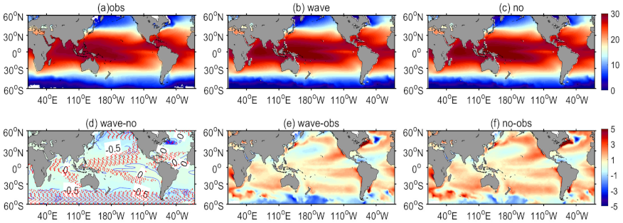
Figure 1. Climatological SST ( ) in (a) observational data, (b) wave run simulations, and (c) no-wave run simulations; (d) difference between the wave run and no-wave run simulations, (e) difference between the wave run simulations and the observation, and (f) the difference between the no-wave run simulations and the observation. The points (in (d)) denote the statistically significant difference between wave run and no-wave run at the confidence level of 90%.
Jmse 09 00457 g001
Figure 2. (a) Horizontal climatological surface Bv ( cm 2 / s ), (b) vertical climatological longitude−averaged Bv ( cm 2 / s ), and (c) vertical climatological longitude−average ocean temperature ( ).
Jmse 09 00457 g002
Figure 3. Nino3 vs. Nino4 indices during the boreal winter (DJF) of El Niño events in the observation (red), wave run simulations (green), and no−wave run simulations (blue).
Jmse 09 00457 g003
Figure 4. Standard deviation of SST anomalies ( averaged within the Niño 3 region in each month for the observation (blue), wave run simulations (red), and no-wave run simulations (yellow).
Jmse 09 00457 g004
Figure 5. Nino 3 index spectra for the observation (green), wave run simulations (red), and no-wave run simulations (blue).
Jmse 09 00457 g005
Figure 6. Distribution SST anomaly patterns ( ) of (ac) ENSO warm phase and (AC) cold phase in the observation, wave run simulations, and no−wave run simulations; and (d,e,D,E) their differences.
Jmse 09 00457 g006
Figure 7. El Niño composites in no−wave run simulations (left column), wave run simulations (middle column) and the observation (right column). Time−longitude evolution of (ac) surface zonal wind stress anomalies (TAUXA, dyne / cm 2 ), (df) thermocline depth anomalies (D20A, m ) and (gi) SSTA ( ) in the composites. The points (in middle column) denote the statistically significant difference between wave run and no−wave run at the confidence level of 90%.
Jmse 09 00457 g007
Figure 8. La Niña composites in no−wave run simulations (left column), wave run simulations (middle column) and the observation (right column). Time−longitude evolution of (ac) surface zonal wind stress anomalies (TAUXA, dyne / cm 2 ), (df) thermocline depth anomalies (D20A, m ) and (gi) SSTA ( ) in the composites. The points (in middle column) denote the statistically significant difference between wave run and no−wave run at the confidence level of 90%.
Jmse 09 00457 g008
Figure 9. Oceanic mixed layer heat budget during La Niña events based on the no−wave run (blue) and wave run (red) simulations. U, V, W, and T represent the zonal advection, meridional advection, vertical advection, and temperature anomaly tendency, respectively ( / month ). The black bars denote one standard deviation.
Jmse 09 00457 g009
Publisher’s Note: MDPI stays neutral with regard to jurisdictional claims in published maps and institutional affiliations.